Article

Updating of Land Cover Maps and Change Analysis Using GlobeLand30 Product: A Case Study in Shanghai Metropolitan Area, China

1
College of Surveying and Geo-Informatics, Tongji University, 1239 Siping Road, Shanghai 200092, China
2
College of Life Sciences and Oceanography, Shenzhen University, Shenzhen 518060, China
*
Author to whom correspondence should be addressed.
Remote Sens. 2020, 12(19), 3147; https://doi.org/10.3390/rs12193147
Submission received: 18 July 2020 / Revised: 3 September 2020 / Accepted: 20 September 2020 / Published: 24 September 2020
(This article belongs to the Special Issue Urban Land Use Mapping and Analysis in the Big Data Era)

Abstract

:
Accurate land cover mapping and change analysis is essential for natural resource management and ecosystem monitoring. GlobeLand30 is a global land cover product from China with 30 m resolution that provides reliable data for many international scientific programs. Few studies have focused on systematically implementing this global land cover product in regional studies. Therefore, this paper presents an object-based extended change vector analysis (ECVA_OB) and transfer learning method to update the reginal land cover map using GlobeLand30 product. The method is designed to highlight small and subtle changes through the concept of uncertain area analysis. Updating is carried out by classifying changed objects using a change-detection-based transfer learning method. Land cover changes are analyzed and the factors affecting updating results are explored. The method was tested with data from Shanghai, China, a city that has experienced significant changes in the past decade. The experimental results show that: (1) the change detection and classification accuracy of the proposed method are 83.30% and 78.77%, respectively, which are significantly better than the values obtained for the multithreshold change vector analysis (MCVA) and the multithreshold change vector analysis and support vector machine (MCVA + SVM) methods; (2) the updated results agree well with GlobeLand30 2010, especially for cultivated land and artificial surfaces, indicating the effectiveness of the proposed method; (3) the most significant changes over the past decade in Shanghai were from cultivated land to artificial surfaces, and the total area containing artificial surfaces in Shanghai increased by about 55% from 2000 to 2011. The factors affecting the updating results are also discussed, which be attributed to the classification accuracy of the base image, extended change vector analysis, and object-based image analysis.

Graphical Abstract

1. Introduction

With the rapid growth of the global population and economic developments, urbanization has taken place at an unprecedented rate all over the world [1]. The extent of this urbanization is constantly increasing, resulting in land use and land cover types undergoing dramatic changes all over the world. Accurate land cover mapping and change analysis are of great importance to natural resource management [2,3], ecosystem monitoring [4], urban planning [1], sustainable development [5], and other social aspects [6,7]. Remotely sensed data can provide repeat observations of most of the Earth’s surface over the long term. As such, remote sensing is considered an effective tool for large-scale land cover mapping and change analysis [8,9,10,11,12,13,14]. Many global land cover products have been established, such as the University of Maryland land cover dataset (UMD) [8]; DIScover [15]; Moderate-resolution Imaging Spectroradiometer (MODIS) land cover product (MOD12) [16,17]; Global Land Cover Database for the Year 2000 (CLC2000) [18]; GlobeCover 2009 [19]; Global Land Cover by National Mapping Organizations (GLCNMO) [20]; and GlobeLand30 [21]. These products have provided reliable data for a series of international scientific research programs. To maintain the value of existing land cover products, consistent and timely updating is essential.
Land cover maps and databases are generally updated through remote sensing imagery by either entire updating or local updating. Entire updating is applied to the whole land cover map by means of data acquisition, pre-processing, and production. Remote-sensing-based image classification is the key, and auxiliary data are usually involved. For example, the National Land Cover Database (NLCD) for the year 1992 was the first regional 30 m resolution land cover product for the United States [22]. An unsupervised classification strategy was implemented for NLCD 1992. The NLCD 2001 used the decision tree algorithm to classified the images. This included three thematic layers, namely land cover, percent imperviousness, and percent tree canopy [23,24]. The Chinese government started work on a global land cover (GLC) mapping program in 2010, aiming to produce a global GLC product at 30 m resolution (GlobeLand30) for the years 2000 and 2010. To achieve this, an automatic classification method, called the pixel-object-knowledge (POK)-based approach, was implemented independently for these two datasets [21]. Yu et al. [25] improved the finer resolution observation and monitoring of global land cover (FROM-GLC) using time-series MODIS data, with the aid of bioclimatic data, a digital elevation model (DEM), and a soil–water conditions map. To improve the accuracy, a spatial temporal sample selection criterion and two classifiers were applied. In entire updating, the land cover map is reclassified independently, which can avoid the cumulative error of the previous land cover map. However, this method often involves large-scale data acquisition and processing, which are both labor- and cost-intensive, and can take five years from image acquisition to product release [1,2]. The land cover can undergo dramatic changes during production in some regions, which greatly affects the effectiveness of the product.
Local updating has been proposed to address these issues, where only the changed areas are updated. Image-based change detection often involves local updating, which significantly reduces the production period and cost. Reliable training samples can be obtained from the unchanged areas by transfer learning. Transfer learning or domain adaption uses the available information in the source domain to classify the target domain, providing a good solution to the problem of insufficient training samples [26]. For example, Xian et al. [2] developed a multithreshold change vector analysis (MCVA) method to extract the changes, and they updated the NLCD from 2006 to 2011. The advantages of this method are that it considers the change magnitude variation of the different kinds of land covers and can satisfactorily and cost-effectively update the land cover map. As a result, it has been adopted in a number of studies [27]. However, this method uses change magnitude as the only feature to extract change information, which often leads to underextraction. An automatic approach was proposed to update land cover maps utilizing integrated change detection and classification methods. Changed information was extracted using a change vector analysis based on posterior probability (CVAPS) and post-classification comparison [11]. Jin et al. [28] proposed a multi-index integrated change analysis (MIICA) model to extract changes and used it to update the NLCD from 2006 to 2011. The Alaska NLCD was updated from 2001 to 2011 and the changes were described with different drivers [29]. Hu et al. [30] combined CVAPS and normalized difference vegetation index (NDVI) data to update GlobeCover 2009 to 2014. The land cover maps were renewed by relational knowledge transfer from GlobeLand30, where transfer learning samples were optimized by indices and auxiliary data [31]. In addition, a number of change-detection-based updating methods for small areas have been proposed, such as reweighted multivariate iteration detection, change-detection-driven transfer learning (CDTL), and domain adaption [26,27,28,29,30,31,32,33,34].
Great progress has been achieved in land cover updating, but some issues still remain: (1) Land cover mapping over large and especially rapidly urbanizing regions is extraordinarily difficult because of inter-scene variability [35], lack of sufficient training samples, and diversity of land cover types. Strategies are needed to decrease the confusion between land cover types. (2) Traditional change detection methods struggle with small and subtle changes due to the use of the mean spectral difference in change vector analysis (CVA) and the complexity of changes over large areas. Hence, some methods suitable for small areas lead to underextraction in large areas. It is critical to improve the extraction of small and subtle changes. (3) The global existing land cover products, e.g., GlobeLand30, have provided reliable data for global change research. Few studies have focused on systematically implementing the existing global land cover products in regional land cover updating studies. Comprehensive research and an analysis of the factors affecting the land cover updating results are needed.
The current paper presents a novel method for updating the land cover map of Shanghai for the period 2000–2011 and for analyzing the changes during this time period. Three principal issues are investigated: (1) an improved change detection method highlights small and subtle changes so as to resolve the problem of underextraction with traditional CVA methods; (2) taking Shanghai as a case study, the land cover map is updated to 2011 using GlobeLand30 2000 as the base map and the problem of land cover confusion over large areas is addressed; (3) the land cover changes and transitions during this period are analyzed.
The remainder of this paper is organized as follows. Section 2 discusses the study area and the datasets we used. Section 3 presents the methodology. An experiment comparing the proposed method to others is conducted, and its results are analyzed in Section 4. Factors affecting the updating results are investigated and discussed in Section 5. We present our conclusions in Section 6.

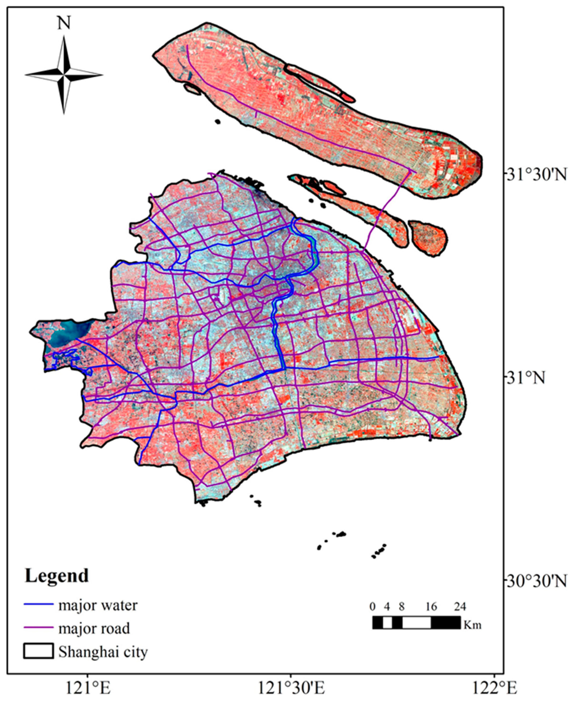
2. Study Area and Data Sets

2.1. Study Area

Shanghai was chosen as the study area. As one of the largest cities in China and a major financial and economic center, it covers an area of about 6340 km2 in the east of the country, between 30°40′N/31°53′N and 120°52′E/122°12′E (Figure 1). The population was about 23.03 million in 2010, and is expected to rise to 28.40 million by 2025 [36]. Table 1 shows the land cover statistical results from GlobeLand30 2000 in Shanghai. It was found that there are five main land cover types, namely cultivated land, grassland, water bodies, wetland, and artificial surfaces. Cultivated land mainly includes paddy fields and dry farm land, which accounts for about 66% of the total area. Forest land is rare and only accounts for less than 0.05% of the total area. The aforementioned five land cover types are enough to constitute the class system for the study area. Therefore, the proposed method only considers the abovementioned five land cover types.
From 2000 to 2011, the Shanghai metropolitan area saw significant land use and land cover (LULC) changes, characterized by the expansion of artificial surfaces and the decrease of cultivated land. Water bodies and wetland areas are also highly dynamic [37]. Therefore, the study area presents a good scenario to test our approach.

2.2. Data Sets

2.2.1. GlobeLand30

GlobeLand30 is a 30 m resolution global land cover dataset consisting of two products: GlobeLand30 2000 and GlobeLand30 2010 [21]. The images are mainly from Landsat Thematic Mapper (TM), Enhanced Thematic Mapper Plus (ETM+), and the Chinese Environmental Disaster Alleviation Satellite (HJ-1). GlobeLand30 implements a POK-based classification approach using a variety of ancillary data, e.g., the existing global land cover products, DEM, and global lake and Wetland databases are used. We used GlobeLand30 2000 as the base map to update and GlobeLand30 2010 as the reference to assess the agreement of the obtained results.

2.2.2. Landsat Imagery
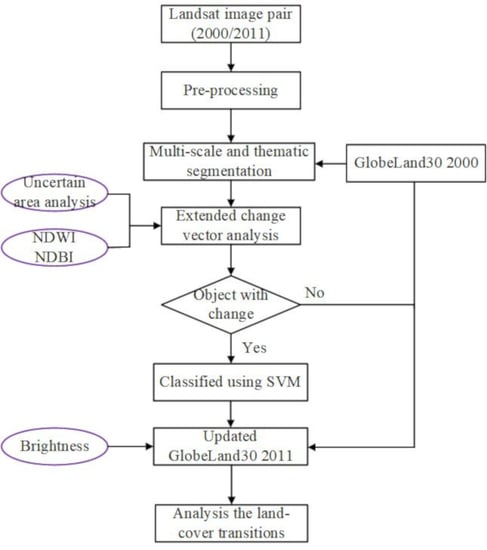
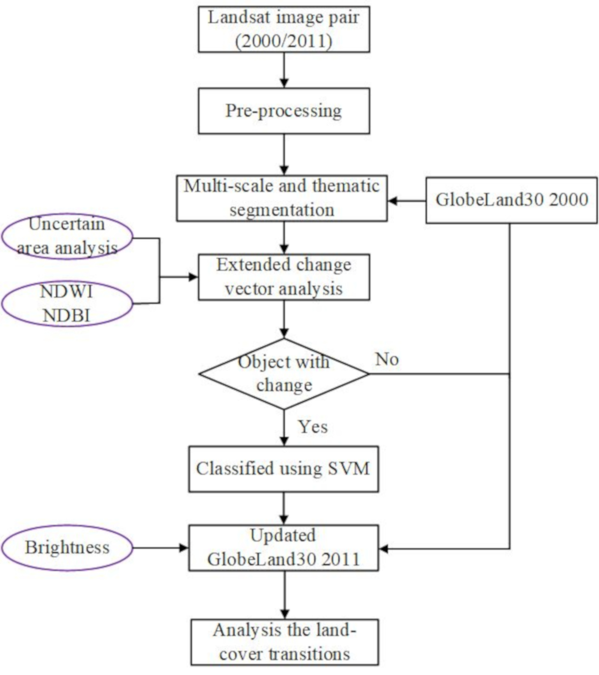
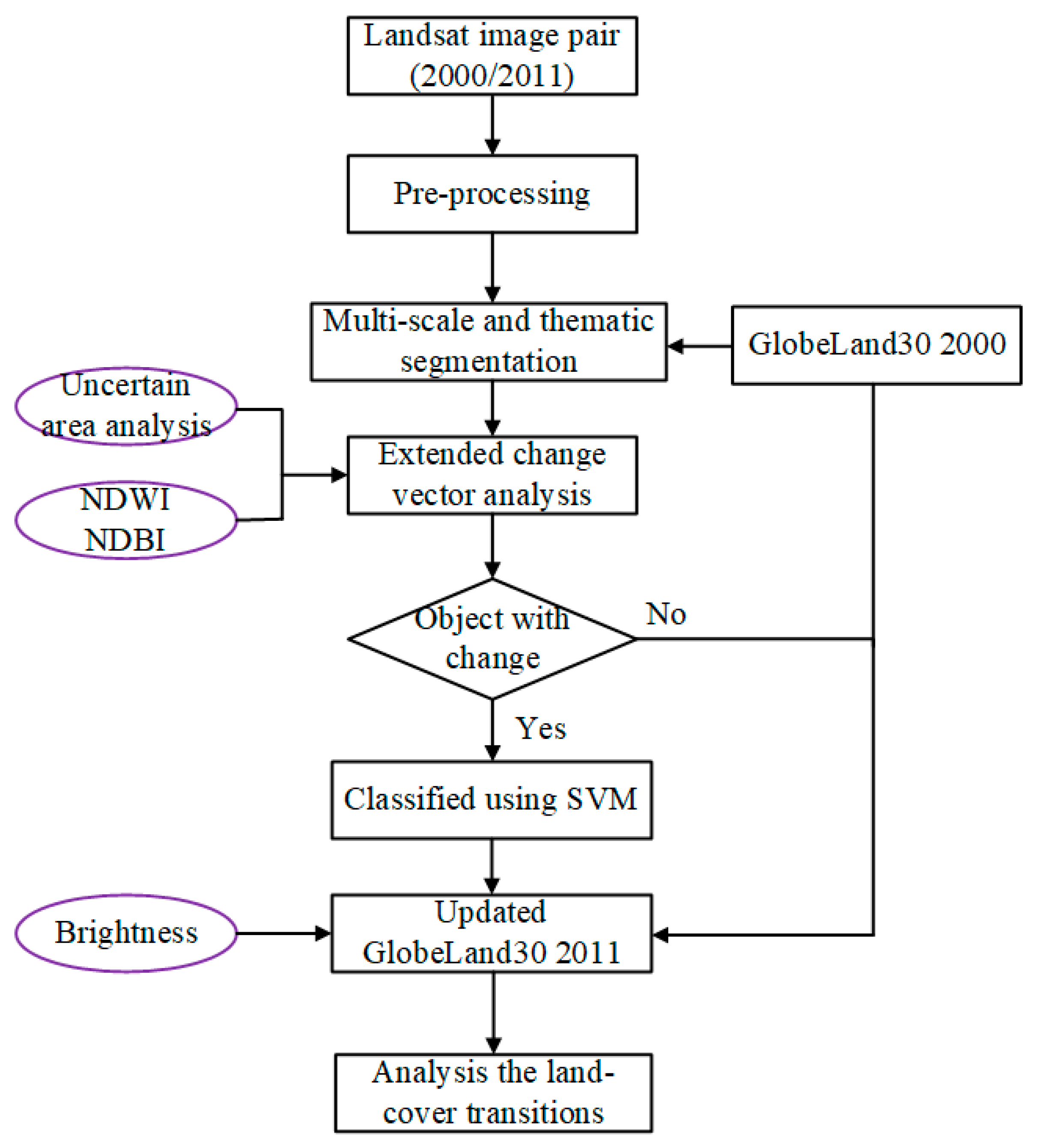
Two scenes of Landsat TM data (118/38 and 118/39) cover the whole administrative area of the city of Shanghai. The remotely sensed data used in GlobeLand30 in Shanghai are from Landsat 7 ETM+. However, there are stripes in the Landsat 7 images due to a scan line corrector (SLC) failure on 31 May 2003; hence, the Landsat 5 TM images with exactly the same spatial resolutions and wavelengths in both the visible and near-infrared bands were selected in this research. These images make a good substitute and they do not require strip repair. After full consideration of the seasonal, phenological, cloud contamination, and temporal coherence issues for GlobeLand30, four scenes of remote sensing images were selected. Table 2 shows information on the images used in the study area, from which it can be seen that temporal gaps are restricted to about a month. For example, for scene 118/38, the Landsat 7 data have the same dates as GlobeLand30 in the year 2000. For scene 118/39 in 2000 and scene 118/38 in 2011, the differences between both are 24 days. However, the data for scene 118/39 in 2011 differ by about three months because no cloud-free image pairs were available. However, this scene accounts for a small part of the city. Overall, the data adopted in this study were consistent with GlobeLand30, and thus provided a good basis for updating and subsequent accuracy verification.

3. Method

The framework of the proposed approach is illustrated in Figure 2, which has the following main steps: (1) data pre-processing involving radiometric and atmosphere corrections, image co-registration, and multiresolution segmentation; (2) change detection with object-based extended change vector analysis (ECVA_OB); (3) updating of GlobeLand30 2000 to 2011; and (4) analysis of the land cover transitions during the past decade.

3.1. Data Pre-Processing and Multiresolution Segmentation

Landsat 5 L1T data with terrain correction were downloaded from https://glovis.usgs.gov/. Atmospheric correction converted the digital number to the top of the atmospheric reflectance [38]. These images were registered with an error of less than 0.5 pixels. Relative radiometric correction eliminated the radiometric differences between multidate satellite images. Among the many relative normalization methods, a linear regression method was selected [1,2]. Images from the year 2000 were normalized to those from 2011 using parameters estimated from 4200 pseudo-invariant feature points.
Multiscale segmentation segmented the images into objects. The segmentation method initialized each pixel as a single segment, and spatially adjacent objects were merged according to the degree of heterogeneity [39]. The iterations stopped when there were no more possible merging steps [40,41,42]. The most important parameters in segmentation were the scale and shape.
As there are great differences in the average sizes of objects in different land cover types, we established a three-level hierarchy of objects by land cover types, with scale parameters of 30, 50, and 100. Grassland is rare and scattered in the study area, so level 1 was designed to detect the changes of grassland. Objects generated at level 2 were prepared to detect changes of water bodies, wetlands, and artificial surfaces, and those at level 3 detected changes of cultivated land. The parameters of color and shape were set to 0.9 and 0.1, respectively, according to previous studies [43,44]. GlobeLand30 2000 served as the thematic layer for segmentation to prevent generated objects from passing through the boundaries of different land cover types [41].

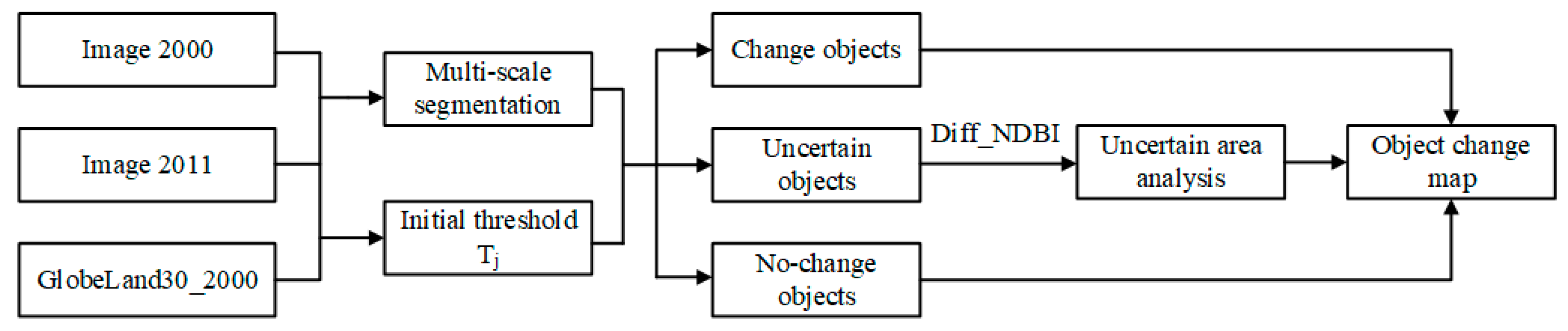
3.2. Change Detection with Extended Change Vector Analysis

Change detection (CD) is supposed to identify changes occurring over the same area at different observation times. It has been extensively applied in LULC monitoring [12,33,45], urban expansion [46,47], ecosystem environment monitoring [4,48], and disaster monitoring [7,49]. Among the current CD methods, CVA is most often used [50]. Assume that R and S are the pixel values of bitemporal images acquired on dates t1 and t2, respectively:
R = [ r 1 r 2 r n ] , S = [ s 1 s 2 s n ] ,
where n is the number of spectral bands. The change vector CV and change magnitude Δ V are defined as [2]:
C V = R S = [ r 1 s 1 r 2 s 2 r n s n ] ,
Δ V = [ ( r 1 s 1 ) 2 + ( r 2 s 2 ) 2 + + ( r n s n ) 2 ] 1 / 2 .
The most critical step of CVA is to identify an optimum threshold to differentiate changed and unchanged pixels. Xian et al. [1,2] proposed a MCVA method to identify changes for different land cover classes. The threshold value for each land cover type is defined by the following constraints [2]:
CV j ( x , y ) = { change if   | Δ V j ( x , y ) | | V ¯ j | + a j σ j no change if   | Δ V j ( x , y ) | < | V ¯ j | + a j σ j ,
where j represents a land cover type, | V ¯ j | and σ j are the mean and standard deviation, respectively, of the change vector for land cover type j, and a j is an adjustable parameter. This method considers the magnitude variation of different land cover types, through which the accuracy of change detection can be greatly improved. However, it uses the change magnitude as the only feature, which often leads to omission errors because the change vector is not sensitive to some land cover change types [28]. Some small and subtle changes might be suppressed by the use of the mean spectral difference. In addition, pixel magnitude values close to the threshold might have higher probabilities of misclassification than those far from it [51,52,53]. More features should be used to highlight small and subtle changes. Therefore, we propose an object-based extended change vector analysis method (ECVA_OB), which exploits the concept of uncertain area analysis, as introduced in our previous research [53]. This study differs from the previous research as follows: (1) Uncertain area analysis based on a single threshold, as proposed in the previous research, is extended to the multithreshold domain. (2) In the previous research, uncertain pixels were determined by the spectral similarity of the bitemporal images, which implies that all land cover changes use the same feature. However, land cover changes may have different characteristics. Hence, some more appropriate features should be selected in accordance with the characteristics of different land cover changes. For instance, we utilized the differences of the normalized difference built-up index (NDBI) to extract the change information for cultivated land. In this way, some small and subtle changes can be highlighted. (3) The analysis unit is extended from the pixel level to the object level for consistency with GlobeLand30 2010. Figure 3 shows the procedures of ECVA _OB.
The ECVA_OB method has two main steps.
Step 1: Calculation of the initial threshold of each land cover type and extraction of the uncertain area:
CV j ( x , y ) = { changed   objects I f   | Δ V j ( x , y ) | ( 1 + t ) T j , unchanged   objects I f   | Δ V j ( x , y ) | ( 1 t ) T j , uncertain   objects I f   ( 1 t ) T j < | Δ V j ( x , y ) | < ( 1 + t ) T j ,
T j = | V ¯ j | + a j σ j
As a result, the objects are categorized as changed, unchanged, or uncertain, according to their change magnitude value. In Equation (5), t is the parameter of the uncertain area, which belongs to [0, 1] and indicates the percentage of uncertain area around the initial threshold T j . We set t to 0.25 according to our previous research [53]. A classification map is required to calculate | V ¯ j | and σ j . GlobeLand30 2000 was used for this purpose. As indicated in Equation (5), changed objects usually correspond to relatively large magnitudes, whereas unchanged objects generally have smaller magnitudes. Uncertain objects usually correspond to small and subtle changes that cause difficulty in detecting change information.
Step 2: Uncertain area analysis. This step aims to select more appropriate features for uncertain objects to highlight subtle change information. The main change in Shanghai from 2000 to 2011 was from cultivated land to artificial surfaces, which accounted for more than 70% of all changes. This change is characterized by a relatively low value of NDBI in the pre-time image and a high value in the post-time image. Thus, by calculating the difference of the NDBI values, where NDBI is calculated as [54]:
NDBI = MIR NIR MIR + NIR
the changes from cultivated land to artificial surfaces can be highlighted and easily extracted using a threshold value. As the changes of other land cover types account for only a small proportion of the total, they can be directly extracted using MCVA. However, the spectral signature of water causes significant differences between bitemporal images, which results in incorrect extraction using this method. Thus, the normalized difference water index is applied to extract water bodies from pre- and post-time images [55]:
NDWI = GREEN NIR GREEN + NIR
Direct comparison is applied to extract the water body changes between the two times. The change map can finally be obtained by integrating the results of the above steps.

3.3. Updating of GlobeLand30 to 2011 by Transfer Learning

To update the land cover map for the period ranging from 2000 to 2011, this required reliable and sufficient training samples to train the classifier to discriminate different land cover types. The labels of unchanged objects were transferred to the updated image as the initial training set. Training samples were automatically generated by the stratified random sample method according to the proportion of each land cover type. The changed objects were classified using SVM and unchanged objects were kept the same as in GlobeLand30 2000. We denote this method as ECVA_OB+SVM in this paper.
The spectral responses of water bodies and wetlands are similar, which often leads to their confusion. The spectral curves of water bodies and wetlands in Figure 4 were extracted from three subareas, each containing 10 samples of these two land cover classes. Figure 5 shows the locations of the three subareas. The average spectral signatures for the water body and wetland classes were calculated. From Figure 4, a significant distinction between water bodies and wetlands is found in the near- and mid-infrared bands. Due to the strong absorption characteristics of water in the near-infrared band, water often corresponds to dark areas in the imagery with low reflectance values. However, wetlands often contain vegetation, which has strong reflectivity in the near-infrared band, leading to higher brightness. This feature can be used to effectively distinguish water bodies and wetlands. As indicated on the right part of Figure 4, water bodies and wetlands were correctly discriminated by the brightness feature. Therefore, objects classified as water bodies or wetlands were reclassified according to their brightness value. An object whose brightness value exceeded the threshold was classified as a wetland area, and otherwise as a water body. The threshold value could be determined by visual inspection.

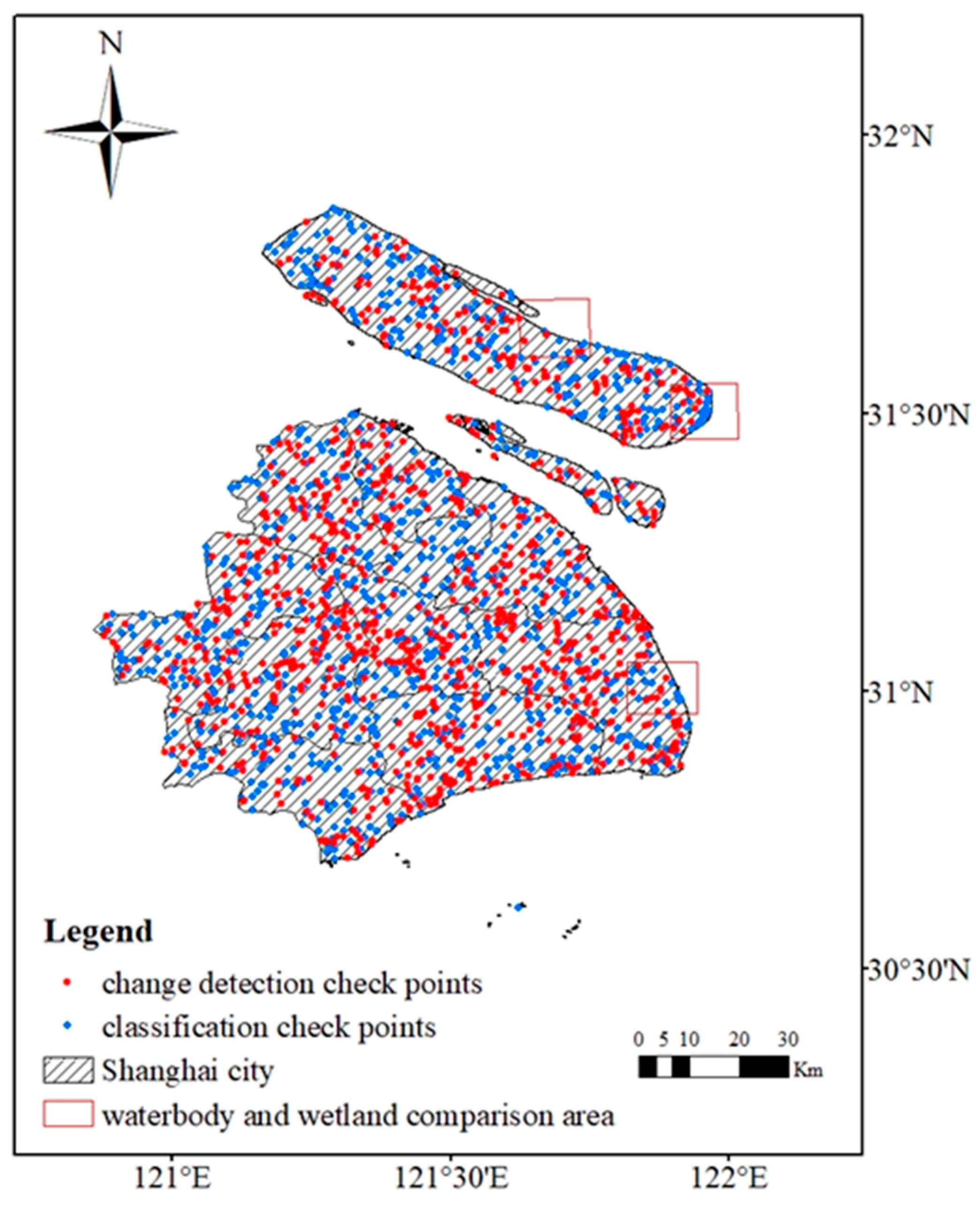
3.4. Accuracy Assessment

Two kinds of check points were generated using the stratified random sample scheme to quantitatively evaluate change detection and classification accuracy [27]. Figure 5 shows the locations of the check points. We selected 1000 check points to assess the change detection accuracy. The percentages of changed and unchanged types were determined by comparing the results of GlobeLand30 2000 and 2010, and 300 changed and 700 unchanged pixels were finally selected. The check points used to assess the classification accuracy for 2011 were chosen based on the percentage of each land cover type in GlobeLand30 2010, with at least 30 samples for each category. In total, 1102 check points were generated to evaluate the updating results. The labels of check points were visually interpreted using remotely sensed images and Google Earth. It should be noted that although the check points are pixel-based, when interpreting the labels of these points, the neighborhood information was also incorporated. Figure 6 shows an example of the check points in the 30 m Landsat imagery and Google Earth.

4. Results

4.1. Results of Change Detection and Method Comparison

The overall change detection accuracy obtained using the ECVA_OB method was 83.30%, with a kappa coefficient of 0.6373 (Table 3). The producer’s accuracy values for unchanged and changed pixels were 80.86% and 89.00%, respectively. Most changes were effectively extracted using the ECVA_OB method. ECVA_OB was also compared to the pixel based multi-threshold change vector analysis method used by Xian et al. [2], which we call MCVA_PB in this paper. The overall accuracy of MCVA_PB was 80.20%, with a kappa coefficient of 0.5185. The producer’s accuracy values for unchanged and changed types were 87.29% and 63.67%, respectively. Among the 300 changed pixels, only 191 were correctly detected, with the other 109 pixels detected as “no change”. Underextraction is a major problem with the MCVA_PB method because it uses the change vector as the only feature to distinguish change from no change. Thus, some small and subtle changes are suppressed when using the mean difference of all the spectral channels of MCVA_PB. However, with the proposed ECVA_OB method, some small and subtle changes that are not sensitive to CVA are defined as uncertain areas and change information can be highlighted by using the selected features. In addition, ECVA_OB effectively incorporates spatial and neighborhood information to avoid the attribute error of an individual pixel and improve the change detection accuracy [47]. Figure 7 shows a more detailed comparison of the results of ECVA_OB and MCVA_PB. As suggested in the figure, MCVA_PB missed a number of changes; hence, the method cannot detect objects with relatively small change magnitudes. It also produces more noise. In contrast, the change detection map derived from ECVA_OB extracts changes more correctly and shows a smoother result.

4.2. Results of Land Cover Classification and Method Comparison

Figure 8a shows the updated land cover map for 2011 obtained by the ECVA_OB+SVM method. The main land cover types for Shanghai in 2011 are cultivated land, water bodies, and artificial surfaces. Wetlands are mainly found in the city’s eastern coastal regions. There are small amounts of grassland. Figure 8c shows the results for GlobeLand30 2010. As shown by the two figures, the proposed method produces distributions similar to GlobeLand30 2010 for each category. Table 4 lists the per-pixel agreements between the generated updating result using ECVA_OB+SVM and GlobeLand30 2010. As suggested from the table, cultivated land and artificial surface agreed well with GlobeLand30 2010 at 83.22% and 78.91%, respectively. The main disagreements for these two land cover types are in the northern and central parts of the image (see Figure 9, rows a and b). In the northern part, the actual land cover types are cultivated land and water bodies. Cultivated land accounts for most of the area, while water bodies are mainly distributed in the central area. However, in this area, GlobeLand30 2010 misclassified cultivated land as water bodies, whereas ECVA_OB+SVM confused cultivated land and artificial surfaces. In the central part, the dominant land cover type is the artificial surface type. The artificial surface area derived by ECVA_OB+SVM was slightly less than that of GlobeLand30 2010. This trend is mainly due to errors in change detection and classification; that is, some objects that had actually changed were detected as no change. As a result, the labels in the base map were transferred to the updated map, which led to errors in the updating result. In addition, some mixed objects composed of cultivated land and artificial surfaces were misclassified as cultivated land, which indicated a smaller artificial surface area than from GlobeLand30 2010. The agreements for wetland and water body areas were 62.20% and 52.26%, respectively. The main disagreement for wetland areas was in the eastern part of the study area (Figure 9, row c), and the main disagreement for water bodies was in the northern part (Figure 9, row a). The water bodies area was significantly over extracted in GlobeLand30 2010. The agreement for grassland was only 15.50% (Figure 9, row d). The grassland areas were both underextracted in the generated updating result and GlobeLand30 2010.
The classification error matrix for 2011 obtained by ECVA_OB+SVM is shown in Table 5. The overall classification accuracy for 2011 was 78.86%, with a kappa coefficient of 0.6608. The producer’s accuracy for cultivated land was 80.24%. Among the 506 check points, 406 were correctly classified. Some cultivated land areas without vegetation cover were classified as artificial surfaces. The producer’s accuracy for grassland was 73.33%. Among the 30 check points for grassland, 22 were correctly classified, with eight pixels misclassified as cultivated land because of the similar spectral signatures of vigorous crops and grassland. Wetland and water bodies showed the best classification results, with producer’s accuracy values of 84.38% and 83.02%, respectively. This is because various auxiliary data, such as the Global Lakes and Wetlands Database (GLWD), were used during classification for GlobeLand30, thus avoiding the omission and misclassification of important wetlands and water bodies. Moreover, brightness information was incorporated to decrease the confusion between water bodies and wetlands, which improved the classification accuracy of these two land cover types. Figure 10 compares the results for water bodies and wetlands before and after incorporating the brightness information. The figure demonstrates that water bodies and wetlands are effectively discriminated using the brightness information. However, some small water bodies were still incorrectly classified, mainly because in GlobeLand30 2000 some small water bodies were merged with cultivated land during segmentation and were subsequently classified as cultivated land. The labels of unchanged water bodies classified as cultivated land in the base map were transferred from GlobeLand30 2000 to 2011, which affected the classification accuracy for the water bodies. Section 5 presents a more detailed discussion of the influence in the base map. The accuracy for artificial surfaces was 76.17%, with the main errors being caused by the confusion of artificial surfaces and cultivated land without crops.
The updating result obtained by ECVA+SVM was also compared to the result from the MCVA_PB+SVM method. To ensure fairness, the decision tree classification algorithm used in Xian et al. [2] was replaced by SVM (denoted as MCVA_PB+SVM) to eliminate the error caused by the classifier. Figure 8b shows the classification result for MCVA_PB+SVM, the overall accuracy of which was 75.95% (Table 6), which was 2.91% lower than that of ECVA_OB+SVM. Compared to the classification results obtained by ECVA_OB+SVM and GlobeLand30 2010, the artificial surfaces obtained using MCVA_PB+SVM were dramatically smaller, especially in the central part of the image. This is largely due to the underextraction of changes in the change detection process. The major land cover changes in Shanghai from 2000 to 2011 were changes from cultivated land to artificial surfaces. If objects with this kind of change are underextracted, then the labels for cultivated land in the base map will be transferred to the updated map, inevitably leading to the decrease of artificial surface areas.

4.3. Results of Land Cover Changes Over the Past Decade

By comparing GlobeLand30 2000 and the classification result for 2011 obtained by the proposed method, the land cover change map for Shanghai over the past 10 years could be generated, as shown in Figure 11. Cultivated land, artificial surfaces, water bodies and Wetlands experienced dramatic changes over those 10 years. The development of artificial surfaces occurred at the cost of cultivated land, water bodies, and Wetlands. Similar conclusions were drawn in Hass et al. [37] and Yin et al. [56] Transformations of cultivated land to artificial surfaces, water bodies to cultivated land, water bodies to artificial surfaces, and wetlands to artificial surfaces accounted for about 92.07% of the changes. Changes from cultivated land to artificial surfaces accounted for 72.76% of the total, and the total area containing artificial surfaces significantly increased by about 51.11% due to urban expansion. Changes from water bodies to cultivated land are mainly seen in Chongming Island and the southeastern coastal area, and account for 7.56% of the total. Changes from water bodies and wetlands to artificial surfaces account for 9.17% and 2.58%, respectively, of the changes, and are mainly seen in the southeastern coastal area.
The multiclass change accuracy was also evaluated using the check points from the changed pixels. The change types of the check points were identified by visual interpretation of the bitemporal images, with the aid of Google Earth images. The percentages of each change type were determined according to the comparison results from GlobeLand30 2000 and 2010. In total, 300 check points were selected, involving four types of land cover transitions. Table 7 lists the multiclass change accuracy. There were 237 changes from cultivated land to artificial surfaces, eight from cultivated land to water bodies, 25 from water bodies to cultivated land, and 30 from water bodies to artificial surfaces. The overall accuracy of the multiple change detection was 75.67%. Changes from cultivated land to artificial surfaces gave the best result, with an accuracy value of 81.43%. Among the 237 check points for the changes from cultivated land to artificial surfaces, 193 pixels were correctly detected and 44 pixels were detected as no change. The errors were mainly due to misclassification of land cover types in 2011. Changes from water bodies to artificial surfaces also showed satisfactory results, with a class detection accuracy of 70.00%. Among the 30 check points for this change type, 21 were correctly detected. Eight of the errors were mainly due to misclassification of the base map, while one was due to the misclassification of the image for the year 2011. The accuracy for the changes from cultivated land to water bodies was only 25%, and among the eight check points only two pixels were correctly detected, with six detected as no change. This low accuracy was mainly caused by the misclassification of the base map and the updating results. The accuracy for the changes from water bodies to cultivated land was 44%, with 11 of 25 pixels detected correctly. The other 14 pixels were incorrectly detected due to misclassification of the post-time image.
In addition, the multiclass change accuracy generated by directly comparing GlobeLand30 2000 and 2010 was also calculated. The overall multiclass accuracy using GlobeLand30 2000 and 2010 was 79.67% (Table 8), which was a little higher than that of the proposed method. Specifically, the accuracy of changes from cultivated land to artificial surfaces and from water to artificial surfaces with the use of GlobeLand30 products was significantly higher than with the proposed method. This was mainly due to the confusion between cultivated areas with no crops and artificial surfaces with the proposed method. Post-classification processing was implemented when producing GlobeLand30, which improved the accuracy of the product. However, the proposed method is completely automatic.

5. Discussion

To analyze the factors that affect the updating results, different components involved in the updating process were analyzed and their influences were evaluated. The factors affecting the updating results are the accuracy of the base map, the extended change vector analysis, and the object-based image analysis.

5.1. The Influence of the Accuracy of the Base Map on Updating

Unlike the entire updating method, which independently produces the land cover map, the proposed method only updates the changed objects. This means that the labels for unchanged pixels that were classified incorrectly in the base map will be transferred to the updated map. The unchanged region usually accounts for a large proportion of the total area. Hence, the overall accuracy of the base map has a tremendous impact on the final updating results. In this study, GlobeLand30 2000 was used as the base map. The influence of GlobeLand30 2000 can be observed in Figure 12. From the first two rows, it can be seen that some of the water bodies were classified as cultivated land in GlobeLand30 2000, and these water bodies remained unchanged. Therefore, the wrong labels were transferred to the year 2011. Rows h, i, and j are examples of the misclassification of artificial surfaces in the base map. As seen in the figure, artificial surfaces were classified as cultivated land in the base map, which resulted in misclassification of the updating results. These errors were mainly caused by the relatively large-scale segmentation parameters when producing GlobeLand30.

5.2. Influence of ECVA on Updating

ECVA is the core module of the proposed method. To determine its contribution, MCVA was carried out at the object level (denoted as MCVA_OB) for comparison with ECVA_OB. The binary change detection result for MCVA_OB is shown in Table 9. The producer’s accuracy for no change was 81.43%, which was 0.57% higher than for ECVA_OB. However, the accuracy for the changed type was only 74.67%, which is 14.33% less than for ECVA_OB. Only 224 of the 300 changed pixels were correctly detected. The overall accuracy of MCVA_OB was 79.40%. By using ECVA, the overall accuracy was improved to 83.30% (Table 3). The main difference was due to the detection accuracy of the changed pixels. Even though the object-based method is incorporated in MCVA, some small and subtle changes still could not be correctly extracted, which led to underextraction of the change information. However, in the ECVA_OB method, small and subtle changes are defined as uncertain areas, which are analyzed by features that can highlight the change information. As a result, the accuracy of the change detection was greatly improved. In addition, the classification result based on integration of MCVA_OB and SVM (MCVA_OB+SVM) for 2011 was generated using the same classification scheme, where only the changed regions were reclassified. Table 6 shows the comparison result. The classification accuracy for 2011 using MCVA_OB+SVM was 78.13%, which was 0.73% lower than for ECVA_OB+SVM. It should be noted that in this study, uncertain area analysis was only used to extract the changes for cultivated land, because these accounted for more than 70% of the changes. However, this idea is suitable for all land cover types if proper features are chosen.

5.3. Influence of Object-Based Analysis on Updating

Object-based image analysis can effectively incorporate spatial and textural features and neighborhood information, which can avoid the attribute errors of a single pixel. To analyze the contribution of object-based analysis, the pixel-based method was carried out using the proposed ECVA method, i.e., the combination denoted as ECVA_PB. The result is shown in Table 10. The producer’s accuracy for no change was 82.71%, which is slightly higher than ECVA_OB. Among the 700 unchanged pixels, 579 were correctly detected. The accuracy for the changed type was 79.67%. Compared to the 89.00% obtained with ECVA_OB, the producer’s accuracy significantly decreased by about 10%. Table 6 compares the results for ECVA_OB and ECVA_PB. It can be observed from the table that the binary change detection accuracy and classification accuracy were both improved by the proposed object-based analysis method. This could be due to the following aspects. First, the object-based method effectively incorporates spatial and neighborhood information. Compared to the pixel-based method, which uses the spectral signature of a single pixel, the object-based method uses the mean spectral feature of the objects, which can avoid the attribute error of a single pixel. Second, spatial registration errors can be reduced by the object-based approach. Registration error critically affects the accuracy of change detection [57,58]. If the registration error is less than 0.5 pixels, then false changes can be reduced [59]. In this study, GlobeLand30 2000 served as a thematic layer during segmentation, resulting in consistent boundaries between data layers for 2000 and 2011.

6. Conclusions

We have proposed an approach to update the land cover maps using a remote-sensing-based change detection and transfer learning method based on GlobeLand30 2000. The method was successfully applied in the rapidly urbanizing city of Shanghai. The experimental results indicated that satisfactory results can be achieved with the proposed method. Compared to state-of-the-art methods, ECVA_OB had superior accuracy. In addition, Shanghai has experienced significant land cover changes over the past 10 years, characterized by changes from cultivated land to artificial surfaces. The factors affecting the updating were also explored, which can be attributed to the accuracy of the base map (GlobeLand30 2000), extended change vector analysis, and object-based image analysis.
Our main contribution is putting forward an approach that applies the global land cover product to regional land cover updating studies, which will be of great importance in order to understand and monitor land cover changes and promote sustainable development. The main idea of the proposed method could be applied to other areas and other regional or global land cover products. Although the strategy of local updating is promising, the classification error of the previous land cover product carries over to the updated product, which is the main limitation of this method. Therefore, we will devote our future research to the design of a scheme that can correct errors in the previous land cover product and improve the updating accuracy.

Author Contributions

Conceptualization, H.P. and X.T.; methodology, H.P.; validation, X.X., X.L., and B.L.; formal analysis, X.L., Y.J., and H.X.; writing—original draft preparation, H.P.; writing—review and editing, X.X. and X.L.; supervision, H.X. All authors have read and agreed to the published version of the manuscript.

Funding

This research was funded by the National Key R&D Program of China (project nos. 2018YFB0505400) and the National Natural Science Foundation of China (project nos. 41631178, 41601414, 41971299, and 41822106).

Conflicts of Interest

The authors declare no conflict of interest.

References

  1. Huang, X.; Wen, D.W.; Li, J.Y.; Qin, R.J. Multi-level monitoring of subtle urban changes for the megacities of China using high-resolution multi-view satellite imagery. Remote Sens. Environ. 2017, 56, 56–75. [Google Scholar] [CrossRef]
  2. Xian, G.; Homer, C.; Fry, J. Updating the 2001 national land cover database land cover classification to 2006 by using Landsat imagery change detection methods. Remote Sens. Environ. 2009, 113, 1133–1147. [Google Scholar] [CrossRef] [Green Version]
  3. Hansen, M.C.; Loveland, T.R. A review of large area monitoring of land cover change using Landsat data. Remote Sens. Environ. 2012, 122, 66–74. [Google Scholar] [CrossRef]
  4. Coppin, P.; Jonckheere, I.; Nackaerts, K.; Muys, B. Digital change detection methods in ecosystem monitoring: A review. Int. J. Remote Sens. 2004, 10, 1565–1596. [Google Scholar] [CrossRef]
  5. Foley, J.A.; Defries, R.; Asner, G.P.; Barford, C.; Bonan, G.; Carpenter, S.R.; Chapin, F.S., III; Coe, M.T.; Daily, G.C.; Gibbs, H.; et al. Global consequences of land use. Science 2005, 309, 570–574. [Google Scholar] [CrossRef] [PubMed] [Green Version]
  6. Zell, E.; Huff, A.K.; Carpenter, A.T.; Friedl, L.A. A user-driven approach to determining critical earth observation priorities for societal benefit. IEEE J. Sel. Top. Appl. Earth Obs. Remote Sens. 2012, 5, 1594–1602. [Google Scholar] [CrossRef]
  7. Lu, P.; Qin, Y.Y.; Li, Z.B.; Mondini, A.C.; Casagli, N. Landslide mapping from multi-sensor data through improved change detection-based Markov random field. Remote Sens. Environ. 2019, 231, 111235. [Google Scholar] [CrossRef]
  8. Hansen, M.C.; Defries, R.S.; Townshend, J.R.G.; Sohlberg, R. Global land cover classification at 1 km spatial resolution using a classification tree approach. Int. J. Remote Sens. 2000, 21, 1331–1364. [Google Scholar] [CrossRef]
  9. Zhang, X.; Sun, R.; Zhang, B.; Tong, Q.X. Land cover classification of the north china plain using MODIS_EVI time series. ISPRS-J. Photogramm. Remote Sens. 2008, 63, 476–484. [Google Scholar] [CrossRef]
  10. Sulla-Menashe, D.; Friedl, M.A.; Krankina, O.N.; Baccini, A.; Woodcock, C.E.; Sibley, A.; Sun, G.; Kharuk, V.; Elsakov, V. Hierarchical mapping of northern Eurasian land cover using MODIS data. Remote Sens. Environ. 2011, 115, 392–403. [Google Scholar] [CrossRef]
  11. Chen, X.H.; Chen, J.; Shi, Y.S.; Yamaguchi, Y. An automated approach for updating land cover maps based on integrated change detection and classification methods. ISPRS-J. Photogramm. Remote Sens. 2012, 71, 86–95. [Google Scholar] [CrossRef]
  12. Hansen, M.C.; Potapov, P.V.; Moore, R.; Hancher, M.; Turubanova, S.A.; Tyukavina, A.; Thau, D.; Stehman, S.V.; Loveland, T.R.; Kommareddy, A.; et al. High-resolution global maps of 21st-century forest cover change. Science 2013, 342, 851–853. [Google Scholar] [CrossRef] [PubMed] [Green Version]
  13. Costa, H.; Carrao, H.; Bação, F.; Caetano, M. Combining per-pixel and object-based classifications for mapping land cover over large areas. Int. J. Remote Sens. 2014, 35, 738–753. [Google Scholar] [CrossRef]
  14. Liu, X.; Hu, G.; Chen, Y.; Li, X.; Xu, X.; Li, S.; Pei, F.; Wang, S. High-resolution multi-temporal mapping of global urban land using Landsat images based on the Google Earth Engine Platform. Remote Sens. Environ. 2018, 209, 227–239. [Google Scholar] [CrossRef]
  15. Loveland, T.R.; Reed, B.C.; Brown, J.F.; Ohlen, D.O.; Zhu, Z.; Yang, L.; Merchant, J.W. Development of a GLC characteristics database and IGBP discover from 1 km AVHRR data. Int. J. Remote Sens. 2000, 21, 1303–1330. [Google Scholar] [CrossRef]
  16. Friedl, M.A.; McIver, D.K.; Hodges, J.C.F.; Zhang, X.Y.; Muchoney, D.; Strahler, A.H.; Woodcock, C.E.; Gopal, S.; Schneider, A.; Cooper, A.; et al. Global land cover mapping from MODIS: Algorithms and early results. Remote Sens. Environ. 2002, 83, 287–302. [Google Scholar] [CrossRef]
  17. Friedl, M.A.; Sulla-Menashe, D.; Tan, B.; Schneider, A.; Ramankutty, N.; Sibley, A.; Huang, X. MODIS collection 5 global land cover: Algorithm refinements and characterization of new datasets. Remote Sens. Environ. 2010, 114, 168–182. [Google Scholar] [CrossRef]
  18. Bartholomé, E.; Belward, A.S. GLC2000: A new approach to GLC mapping from earth observation data. Int. J. Remote Sens. 2005, 26, 1959–1977. [Google Scholar] [CrossRef]
  19. Bontemps, S.; Defourney, P.; Bogaert, E.V.; Arino, O.; Kalogirou, V.; Perez, J.R. GlobCover2009 Products Description and Validation Report. 2010. Available online: http://due.esrin.esa.int/globcover/LandCover2009/GLOBCOVER2009_Validation_Report_2.2.pdf (accessed on 6 August 2019).
  20. Tateishi, R.; Uriyangqai, B.; Al-Bilbisi, H.; Ghar, M.A.; Tsend-Ayush, J.; Kobayashi, T.; Kasimu, A.; Hoan, N.T.; Shalaby, A.; Alsaaideh, B.; et al. Production of global land cover-GLCNMO. Int. J. Digit. Earth. 2011, 4, 22–49. [Google Scholar] [CrossRef]
  21. Chen, J.; Chen, J.; Liao, A.; Cao, X.; Chen, L.; Chen, X.; He, C.; Han, G.; Peng, S.; Lu, M.; et al. Global land cover mapping at 30 m resolution: A POK-based operational approach. ISPRS-J. Photogramm. Remote Sens. 2014, 103, 7–27. [Google Scholar] [CrossRef] [Green Version]
  22. Vogelmann, J.; Howard, S.M.; Yang, L.M.; Larson, C.R.; Wylie, B.K.; Van Driel, N. Completion of the 1990′s National Land Cover Data Set for the conterminous United States from Landsat Thematic Mapper data and ancillary data sources. Photogramm. Eng. Remote Sens. 2001, 67, 650–662. [Google Scholar]
  23. Homer, C.; Dewitz, J.; Fry, J.; Coan, M.J.; Hossain, N.; Larson, C.; Herold, N.; McKerrow, A.J.; VanDriel, J.N.; Wickham, J. Completion of the 2001 National Land Cover Database for the conterminous United States. Photogramm. Eng. Remote Sens. 2007, 73, 337–341. [Google Scholar]
  24. Homer, C.; Dewitz, J.; Yang, L.M.; Jin, S.M.; Danielson, P.; Xian, G.; Coulston, J.; Herold, N.; Wickham, J.; Megown, K. Completion of the 2011 national land cover database for the conterminous United States-representing a decade of land cover change information. Photogramm. Eng. Remote Sens. 2015, 81, 345–354. [Google Scholar]
  25. Yu, L.; Wang, J.; Gong, P. Improving 30 m global land-cover map FROM-GLC with time series MODIS and auxiliary data sets: A segmentation-based approach. Int. J. Remote Sens. 2013, 34, 5851–5867. [Google Scholar] [CrossRef]
  26. Bruzzone, L.; Marconcini, M. Toward the automatic updating of land-cover maps by a domain-adaptation SVM classifier and a circular validation strategy. IEEE Trans. Geosci. Remote Sens. 2009, 1108–1122. [Google Scholar] [CrossRef]
  27. Yu, W.J.; Zhou, W.Q.; Qian, Y.G.; Yan, J.L. A new approach for land cover classification and change analysis: Integrating backdating and an object-based method. Remote Sens. Environ. 2016, 177, 37–47. [Google Scholar] [CrossRef]
  28. Jin, S.M.; Yang, L.M.; Danielson, P.; Homer, C.; Fry, J.; Xian, G. A comprehensive change detection method for updating the national land cover database to circa 2011. Remote Sens. Environ. 2013, 132, 159–175. [Google Scholar] [CrossRef] [Green Version]
  29. Jin, S.M.; Yang, L.M.; Zhu, Z.; Homer, C. A land cover change detection and classification protocol for updating Alaska NLCD 2001 to 2011. Remote Sens. Environ. 2017, 195, 44–55. [Google Scholar] [CrossRef]
  30. Hu, Y.F.; Dong, Y.; Batunacun. An automatic approach for land-change detection and land updates based on integrated NDVI timing analysis and the CVAPS method with GEE support. ISPRS-J. Photogramm. Remote Sens. 2018, 146, 347–359. [Google Scholar] [CrossRef]
  31. Lin, C.; Du, P.J.; Samat, A.; Li, E.Z.; Wang, X.; Xia, J.S. Automatic updating of land cover maps in rapidly urbanizing regions by relational knowledge transferring from GlobeLand30. Remote Sens. 2019, 11, 1397. [Google Scholar] [CrossRef] [Green Version]
  32. Demir, B.; Bovolo, F.; Bruzzone, L. Updating land-cover maps by classification of image time series: A novel change-detection-driven transfer learning approach. IEEE Trans. Geosci. Remote Sens. 2013, 51, 300–312. [Google Scholar] [CrossRef]
  33. Wessels, K.J.; Van den Bergh, F.; Roy, D.P.; Salmon, B.P.; Steenkamp, K.C.; MacAlister, B.; Swanepoel, D.; Jewitt, D. Rapid land cover map updates using change detection and robust random forest classifiers. Remote Sens. 2016, 8, 888. [Google Scholar] [CrossRef] [Green Version]
  34. Wu, T.J.; Luo, J.C.; Zhou, Y.N.; Wang, C.P.; Xi, J.B.; Fang, J.W. Geo-object-based land cover map update for high-spatial-resolution remote sensing images via change detection and label transfer. Remote Sens. 2020, 12, 174. [Google Scholar] [CrossRef] [Green Version]
  35. Ban, Y.F.; Gong, P.; Gini, C. Global land cover mapping using Earth observation satellite data: Recent progresses and challenges. ISPRS-J. Photogramm. Remote Sens. 2015, 103, 1–6. [Google Scholar] [CrossRef] [Green Version]
  36. United Nations. World Urbanization Prospects: The 2011 Revision; United Nations: New York, NY, USA, 2012. [Google Scholar]
  37. Haas, J.; Furberg, D.; Ban, Y.F. Satellite monitoring of urbanization and environmental impacts-a comparison of Stockholm and Shanghai. Int. J. Appl. Earth Obs. Geoinf. 2015, 38, 138–149. [Google Scholar] [CrossRef]
  38. Homer, C.; Huang, C.Q.; Yang, L.M.; Wylie, B.; Coan, M. Development of a 2001 national land-cover database for the United States. Photogramm. Eng. Remote Sens. 2004, 70, 829–840. [Google Scholar] [CrossRef] [Green Version]
  39. Yang, X.Y.; Lo, C.P. Relative radiometric normalization performance for change detection from multi-date satellite images. Photogramm. Eng. Remote Sens. 2000, 66, 967–980. [Google Scholar]
  40. Zhou, W.Q.; Troy, A. An object-oriented approach for analyzing and characterizing urban landscape at the parcel level. Int. J. Remote Sens. 2008, 29, 3119–3135. [Google Scholar] [CrossRef]
  41. Zhou, W.Q.; Troy, A.; Grove, J.M. Object-based land cover classification and change analysis in the Baltimore metropolitan area using multitemporal high resolution remote sensing data. Sensors 2008, 8, 1613–1636. [Google Scholar] [CrossRef] [Green Version]
  42. Blaschke, T. Object based image analysis for remote sensing. ISPRS-J. Photogramm. Remote Sens. 2010, 65, 2–16. [Google Scholar] [CrossRef] [Green Version]
  43. Benz, U.C.; Hofmann, P.; Willhauck, G.; Lingenfelder, I.; Heynen, M. Multi-resolution, object-oriented fuzzy analysis of remote sensing data for GIS-ready information. ISPRS-J. Photogramm. Remote Sens. 2004, 58, 239–258. [Google Scholar] [CrossRef]
  44. Pu, R.L.; Landry, S.; Yu, Q. Object-based urban detailed land cover classification with high spatial resolution IKONOS imagery. Int. J. Remote Sens. 2011, 32, 3285–3308. [Google Scholar] [CrossRef] [Green Version]
  45. He, C.Y.; Wei, A.; Shi, P.J.; Zhang, Q.F.; Zhao, Y.Y. Detecting land-use/land-cover change in rural–urban fringe areas using extended change-vector analysis. Int. J. Appl. Earth Obs. Geoinf. 2011, 13, 572–585. [Google Scholar] [CrossRef]
  46. Li, X.C.; Gong, P.; Liang, L. A 30-year (1984–2013) record of annual urban dynamics of Beijing city derived from Landsat data. Remote Sens. Environ. 2015, 166, 78–90. [Google Scholar] [CrossRef]
  47. Xiao, P.F.; Zhang, X.L.; Wang, D.G.; Yuan, M.; Feng, X.Z.; Kelly, M. Change detection of built-up land: A framework of combining pixel-based detection and object-based recognition. ISPRS-J. Photogramm. Remote Sens. 2016, 119, 402–414. [Google Scholar] [CrossRef]
  48. Desclée, B.; Bogaert, P.; Defourny, P. Forest change detection by statistical object-based method. Remote Sens. Environ. 2006, 102, 1–11. [Google Scholar] [CrossRef]
  49. Li, Z.B.; Shi, W.Z.; Lu, P.; Yan, L.; Wang, Q.M.; Miao, Z.L. Landslide mapping from aerial photographs using change detection-based Markov Random Field. Remote Sens. Environ. 2016, 187, 76–90. [Google Scholar] [CrossRef] [Green Version]
  50. Chen, J.; Gong, P.; He, C.Y.; Pu, R.L.; Shi, P.J. Land-use/land-cover change detection using improved change-vector analysis. Photogramm. Eng. Remote Sens. 2003, 69, 369–379. [Google Scholar] [CrossRef] [Green Version]
  51. Bovolo, F.; Bruzzone, L. A theoretical framework for unsupervised change detection based on change vector analysis in the polar domain. IEEE Trans. Geosci. Remote Sens. 2007, 45, 218–236. [Google Scholar] [CrossRef] [Green Version]
  52. Liu, S.C.; Bruzzone, L.; Bovolo, F.; Du, P.J. Hierarchical unsupervised change detection in multitemporal hyperspectral images. IEEE Trans. Geosci. Remote Sens. 2015, 53, 244–260. [Google Scholar]
  53. Tong, X.H.; Pan, H.Y.; Liu, S.C.; Li, B.B.; Luo, X.; Xie, H.; Xu, X. A novel approach for hyperspectral change detection based on uncertain area analysis and improved transfer learning. IEEE J. Sel. Top. Appl. Earth Obs. Remote Sens. 2020. [Google Scholar] [CrossRef]
  54. Zha, Y.; Gao, J.; Ni, S. Use of normalized difference built-up index in automatically mapping urban areas from TM imagery. Int. J. Remote Sens. 2003, 24, 583–594. [Google Scholar] [CrossRef]
  55. Mcfeeters, S.K. The use of the Normalized Difference Water Index (NDWI) in the delineation of open water features. Int. J. Remote Sens. 1996, 17, 1425–1432. [Google Scholar] [CrossRef]
  56. Yin, J.; Yin, Z.; Zhong, H.; Xu, S.; Hu, X.; Wang, J.; Wu, J. Monitoring urban expansion and land use/land cover changes of Shanghai metropolitan area during the transitional economy (1979–2009) in China. Environ. Monit. Assess. 2011, 9, 1538–1559. [Google Scholar] [CrossRef]
  57. Chen, G.; Zhao, K.G.; Owers, R.P. Assessment of the image misregistration effects on object-based change detection. ISPRS-J. Photogramm. Remote Sens. 2014, 87, 19–27. [Google Scholar] [CrossRef]
  58. Dai, X.L.; Khorram, S. The effects of image misregistration on the accuracy of remotely sensed change detection. IEEE Trans. Geosci. Remote Sens. 1998, 36, 1566–1577. [Google Scholar]
  59. Townshend, J.R.G.; Justice, C.O.; Gurney, C.; Mcmanus, J. The impact of misregistration on change detection. IEEE Trans. Geosci. Remote Sens. 1992, 30, 1054–1060. [Google Scholar] [CrossRef] [Green Version]
Figure 1. Study area in Shanghai, China.
Remotesensing 12 03147 g001
Figure 2. Framework of the proposed method.
Remotesensing 12 03147 g002
Figure 3. Flowchart of object-based extended change vector analysis method (ECVA_OB) method.
Remotesensing 12 03147 g003
Figure 4. Reflectance and brightness values of water bodies and wetlands. (a) the spectral signatures of waterbody and wetland; (b) the brightness of waterbody and wetland.
Remotesensing 12 03147 g004
Figure 5. Distribution map of check points.
Remotesensing 12 03147 g005
Figure 6. Examples of check points in 30 m Landsat imagery and Google Earth.
Remotesensing 12 03147 g006aRemotesensing 12 03147 g006b
Figure 7. Change detection result comparison. Remotely sensed images for (a) 2000 and (b) 2011. (c) Change detection results for the proposed ECVA_OB method and (d) MCVA_PB method.
Remotesensing 12 03147 g007aRemotesensing 12 03147 g007b
Figure 8. Land cover classification maps obtained using different methods: (a) ECVA_OB+SVM; (b) MCVA_PB + SVM; (c) GlobeLand30 2010.
Remotesensing 12 03147 g008
Figure 9. Examples of disagreements between the updating results generated by ECVA_OB+SVM and GlobeLand30 2010.
Remotesensing 12 03147 g009
Figure 10. Comparative results for water bodies and wetlands: (a) remotely sensed image from the year 2011; (b) classification result without using brightness information; (c) classification result using brightness information.
Remotesensing 12 03147 g010
Figure 11. Land cover change map for Shanghai from 2000 to 2011.
Remotesensing 12 03147 g011
Figure 12. Influence of the base map on the updating results: images from (a) 2000 and (b) 2011. (c) Classification map from GlobeLand30 2000. (d) Classification results for 2011 obtained using the proposed ECVA_OB+SVM method.
Remotesensing 12 03147 g012
Table 1. Land cover statistical results from GlobeLand30 2000 in Shanghai.
Land Cover TypesArea (Km2)Percent (%)
Cultivated land4478.6665.88
Forest2.960.04
Grass land18.780.28
Wetland106.141.56
Water bodies396.345.83
Artificial surface1795.0726.41
Table 2. Data used in the study.
YearPath/RowData Used in GlobeLand30Data Used in This Study
SensorDataSensorDate
2000118/38Landsat 72001/07/03Landsat 72001/07/03
118/39Landsat 72000/06/14Landsat 52000/05/21
2011118/38Landsat 72011/04/26Landsat 52011/05/20
118/39Landsat 72011/02/05Landsat 52011/05/20
Table 3. Error matrix and accuracy assessment for binary change detection with ECVA_OB and MCVA_PB methods.
Binary Change Detection Accuracy Assessment for ECVA_OB Method
Classified DataReference DataUser’s acc. (%)
No ChangeChangeTotal
No change5663359994.49
Change 13426740166.58
Total7003001000
Producer’s accuracy (%)80.8689.00
Overall accuracy (%)83.30
Overall kappa statistics0.6373
Binary Change Detection Accuracy Assessment for MCVA_PB Method
Classified DataReference DataUser’s acc. (%)
No ChangeChangeTotal
No change61110972084.86
Change 8919128068.21
Total7003001000
Producer’s accuracy (%)87.2963.67
Overall accuracy (%)80.20
Overall kappa statistics0.5185
Table 4. Per-pixel agreement between generated updating result by ECVA_OB+SVM and GlobeLand30 2010.
Land Cover TypeAgreement (%)
Cultivated land83.22
Grassland15.50
Wetland62.20
Water body52.26
Artificial surface78.91
Table 5. Error matrix and classification accuracy for ECVA_OB+SVM.
Classified DataReference Data User’s Accuracy (%)
Cultivated LandGrasslandWetlandWater BodiesArtificial SurfacesTotal
Cultivated land40682129852677.19
Grassland9220013268.75
Wetland4027103284.38
Water bodies0028839394.62
Artificial surfaces8701532641977.80
Total50630321064281102
Producer’s accuracy (%)80.2473.3384.3883.0276.17
Overall accuracy (%)78.86
Kappa statistics0.6608
Table 6. Comparison of the accuracy of the different methods.
Binary CD MethodAccuracy (%)Classification MethodAccuracy (%)
MCVA_OB79.40MCVA_OB+SVM78.13
MCVA_PB80.20MCVA_PB+SVM75.95
ECVA_PB81.80ECVA_PB+SVM75.86
ECVA_OB83.30ECVA_OB+SVM78.86
Table 7. Multiclass change accuracy of the proposed method.
Classified DataReference Data
Cultivated-ArtificialCultivated-WaterWater-CultivatedWater-Artificial
No change44600
Cultivated–Artificial193021
Cultivated–Water0200
Wetland–Artificial0060
Water–Artificial00218
Water–Cultivated00111
Water–Grass0003
Water–Wetland0002
Total 23783025
Class accuracy (%)81.43257044
Overall accuracy (%)75.67
Table 8. Multiclass accuracy comparison.
Change ClassAccuracy Acquired by Comparing GlobaLand30 2000 and Updated 2011 (%)Accuracy Acquired by Comparing GlobeLand30 2000 and GlobeLand30 2010 (%)
Cultivated–Artificial81.4386.08
Cultivated–Water25.0025.00
Water–Cultivated70.0030.00
Water–Artificial44.0096.00
Overall accuracy (%)75.6779.67
Table 9. Binary change detection error matrix for the MCVA_OB method.
Classified DataReference Data User’s Accuracy (%)
No ChangeChangeTotal
No change5707664688.23
Change13022435463.28
Total7003001000
Producer’s accuracy (%)81.4374.67
Overall accuracy (%)79.40
Overall kappa statistics0.5335
Table 10. Binary change detection error matrix for the ECVA_PB method.
Classified DataReference Data User’s Accuracy (%)
No ChangeChange Total
No change5796164090.47
Change 12123936066.39
Total7003001000
Producer’s accuracy (%)82.7179.67
Overall accuracy (%)81.80
Overall Kappa statistics0.5901

