Article

Remote Sensing Index for Mapping Canola Flowers Using MODIS Data

1
State Key Laboratory of Earth Surface Processes and Resource Ecology, Faculty of Geographical Science, Beijing Normal University, Beijing 100875, China
2
Beijing Engineering Research Center for Global Land Remote Sensing Products, Institute of Remote Sensing Science and Engineering, Faculty of Geographical Science, Beijing Normal University, Beijing 100875, China
3
School of Geography and Information Engineering, China University of Geosciences, Wuhan 430074, China
4
State Environmental Protection Key Laboratory of Satellite Remote Sensing, Aerospace Information Research Institute, Chinese Academy of Sciences, Beijing 100101, China
*
Author to whom correspondence should be addressed.
Remote Sens. 2020, 12(23), 3912; https://doi.org/10.3390/rs12233912
Submission received: 17 October 2020 / Revised: 15 November 2020 / Accepted: 26 November 2020 / Published: 28 November 2020

Abstract

:
Mapping and tracing the changes in canola planting areas and yields in China are of great significance for macro-policy regulation and national food security. The bright yellow flower is a distinctive feature of canola, compared to other crops, and is also an important factor in predicting canola yield. Thus, yellowness indices were previously used to detect the canola flower using aerial imagery or median-resolution satellite data like Sentinel-2. However, it remains challenging to map the canola planting area and to trace long-term canola yields in China due to the wide areal extent of cultivation, different flowering periods in different locations and years, and the lack of high spatial resolution data within a long-term period. In this study, a novel canola index, called the enhanced area yellowness index (EAYI), for mapping canola flowers and based on Moderate Resolution Imaging Spectroradiometer (MODIS) time-series data, was developed. There are two improvements in the EAYI compared with previous studies. First, a method for estimating flowering period, based on geolocation and normalized difference vegetation index (NDVI) time-series, was established, to estimate the flowering period at each place in each year. Second, the EAYI enhances the weak flower signal in coarse pixels by combining the peak of yellowness index time-series and the valley of NDVI time-series during the estimated flowering period. With the proposed EAYI, canola flowering was mapped in five typical canola planting areas in China, during 2003-2017. Three different canola indices proposed previously, the normalized difference yellowness index (NDYI), ratio yellowness index (RYI) and Ashourloo canola index (Ashourloo CI), were also calculated for a comparison. Validation using the samples interpreted through higher resolution images demonstrated that the EAYI is better correlated with the reference canola coverage with R2 ranged from 0.31 to 0.70, compared to the previous indices with R2 ranged from 0.02 to 0.43. Compared with census canola yield data, the total EAYI was well correlated with actual yield in Jingmen, Yili and Hulun Buir, and well correlated with meteorological yields in all five study areas. In contrast, previous canola indices show a very low or even a negative correlation with both actual and meteorological yields. These results indicate that the EAYI is a potential index for mapping and tracing the change in canola areas, or yields, with MODIS data.

Graphical Abstract

1. Introduction

Canola is one of the most important oilseed crops worldwide, and is the primary source of edible oil for human consumption, a high protein meal for livestock, and a renewable biological raw material for the oleochemical industry [1]. Moreover, the ornamental value of canola flowers has also been discovered in China and has largely promoted the local development of tourism agriculture in recent years [2]. Although China is the largest producer of canola in the world [3], domestic production is far from meeting the increasing demand in China. The self-sufficiency rate of canola was only 30.8% in 2017, and the imported amount increased 2–3 fold from 2008 to 2017 [4]. Therefore, mapping and tracing the changes in canola planting areas and yields are of great importance for macro-policy regulation and national food security in China.
Remote sensing is a promising tool for efficiently mapping the areal extent and yield of canola owing to its wide coverage and regular acquisition [5]. The bright yellow flower is a distinctive feature of canola, compared to other crops and vegetation types, and is also an important factor in predicting canola yield [6]. Thus, several previous studies have attempted to detect yellow flowers of canola using remote sensing. For example, Sulik et al. (2015) [6] compared several indices with different band combinations and found that the ratio yellowness index (RYI), calculated as Green/Blue, is well correlated with the flower density of canola. Sulik et al. (2016) [7] further proposed the normalized difference yellowness index (NDYI), computed as (Green − Blue)/(Green + Blue), to predict canola yield. Fang et al. [8] demonstrated that the green band in unmanned aerial vehicle imagery is a good indicator for estimating the flower fraction of canola. These studies show the potential of green and blue bands in detecting the yellow flowers of canola. Moreover, Shen et al. found that yellow flowers could reduce the value of the vegetation index [9,10]. Thus, Tao [11] employed the EVI difference between the flowering stage and the pre-flowering stage to map canola in the Middle Reaches of the Yangtze River Valley. Unfortunately, these indices or features only work for estimating the quantity of flowers in the pixel during the flowering period. Consequently, they cannot be directly used for mapping canola flowers over a large area or in multiple years because the period of flowering differs spatially and temporally. To address this issue, time-series data have been recently employed for detecting the period of flowering [5,12]. Ashourloo et al. [5] identified the inflection point in the Red + Green sequence of Sentinel 2A/B data as the date of flowering and classified canola by thresholding a proposed Canola Index. d’Andrimont et al. [12] employed both the VV-polarized time-series of Sentinel-1, and the NDYI time-series of Sentinel-2, to detect the peak flowering date. The experimental sites were relatively small in these studies, thus cloud-free Sentinel time-series data could be selected. However, the availability of clear Sentinel imagery would become an issue when applying the data over a large area, especially seeing that canola often flowers during the rainy season in China. Supervised classification is another efficient method for canola mapping and detection of the flowering period. Recently, Tao [13] employed an artificial neural network (ANN) model to map canola cultivation in the Jianghan Plain and Dongting Lake Plain, from 2000 to 2017, using Moderate Resolution Imaging Spectroradiometer (MODIS) data. Mercier et al. [14] applied random forest classification to Sentinel-1 and Sentinel-2 data to distinguish the different phenological stages. However, the requirement for a large number of training samples limits its wide application in different areas. In summary, there are several challenges in monitoring changes in canola flowering in China. First, canola cultivars vary across China, with very different flowering periods, ranging from January to August. Such diversity within canola and the mixture with other land-cover types raises the difficulty of detecting the flowering period using time-series data. Second, the Sentinel-2 data employed in recent studies are not available for tracing the historical (prior to 2015) change in canola. Coarse-resolution data, such as MODIS, have a longer-term record. However, it is unknown whether the previously proposed spectral indices are suitable for MODIS because the yellow spectral signal would be relatively weak in coarse pixels. Third, supervised classifications, including ANN or random forest, might work effectively in local areas, but are not suitable for mapping canola flowers across different regions because of the difficulty in collecting a large number of training samples.
To address these issues, a novel index was designed to monitor and quantify canola flowering using MODIS data. There are two improvements compared with previous studies. First, a flowering prediction model, based on geolocation, was established in this study, to restrict the detection of flowering because flowering time varies in a relatively small range at any specific location. Second, an enhanced area yellowness index (EAYI), based on the MODIS time-series, was designed to enhance the weak flower signal in coarse pixels. With the proposed EAYI, canola flowering was mapped in five typical canola planting areas in China, during 2003–2017.

2. Materials and Methods
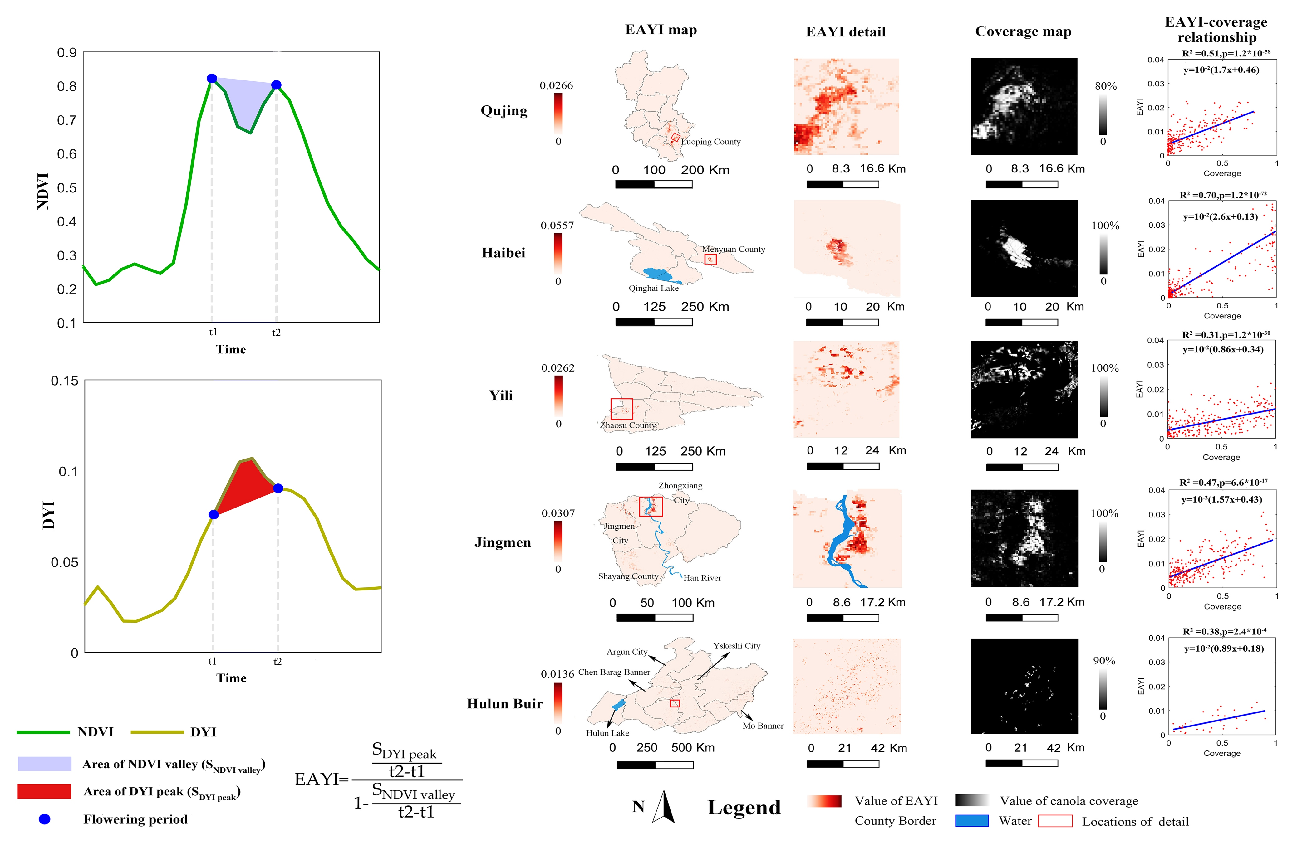
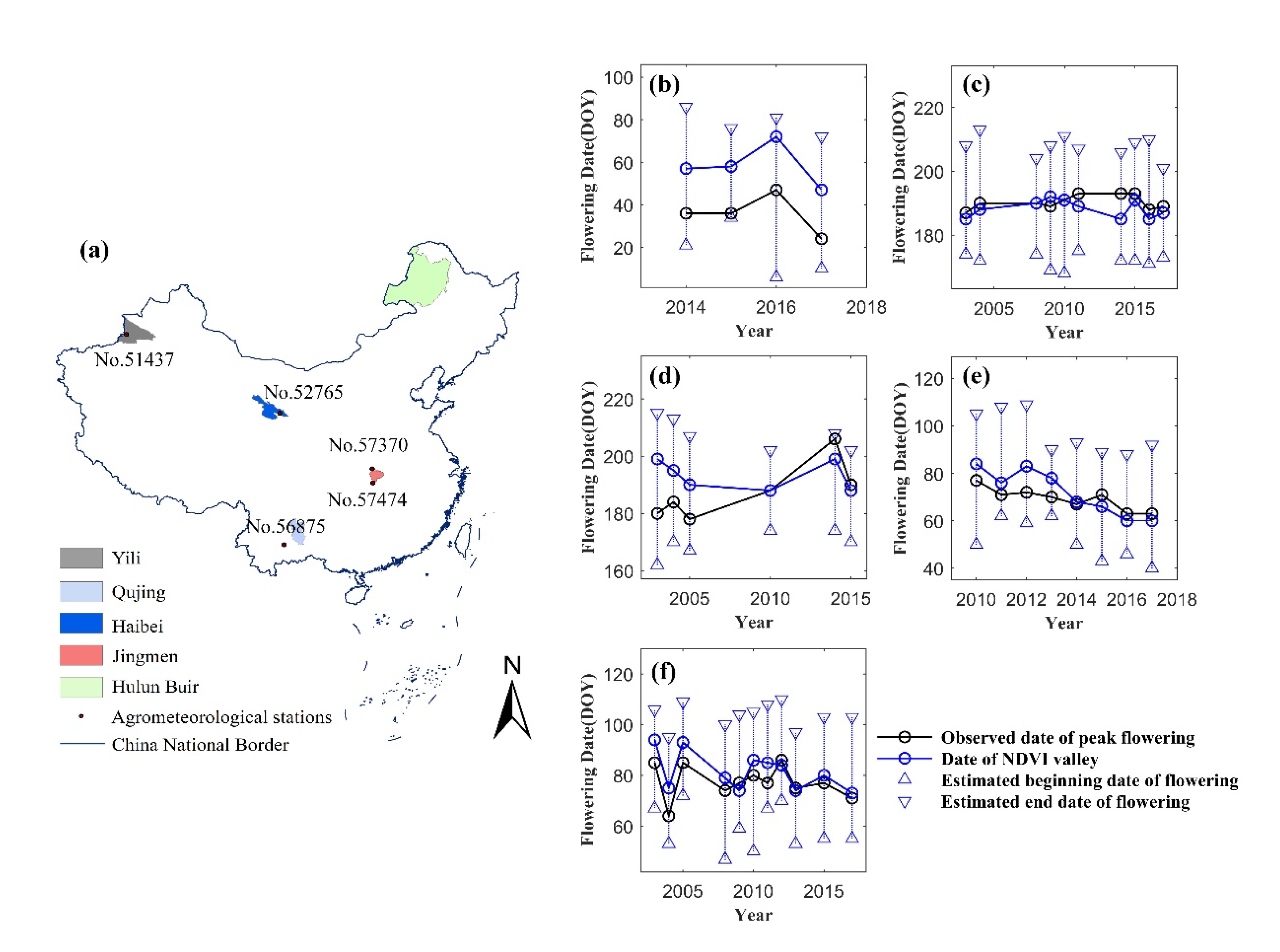
2.1. Study Areas

To validate the proposed EAYI index under various climates in China, five typical prefectures with large canola planting areas, that is, Qujing, Jingmen, Haibei, Yili, and Hulun Buir, were selected as experimental sites (Figure 1) in this study. The selected five areas have very different locations, climates, and canola flowering periods.
Qujing (24°21′–27°03′N, 103°03′–104°49′E) is the largest canola planting prefecture in Yunnan Province [15]. It has a subtropical plateau monsoon climate with an annual average temperature of 15.12 °C and annual precipitation of 944.6 mm. Winter canola in this area is sown in October and flowers from January to February the following year, which is the earliest flowering time of canola in China because of the warm and wet climate.
Jingmen (30°23′–31°37′N, 111°51′–113°29′E) is one of the densest winter canola planting prefectures in the Yangtze River Basin [11]. It has a northern subtropical monsoonal climate, with an annual precipitation of 834.2–894.8 mm and an average temperature of 16.5 °C. Winter canola in this area is sown in November and flowers from March to April of the following year because the temperature in this area is lower than that of Qujing.
Haibei (36°44′–39°05′N, 98°05′–102°41′E) is located in the north of the Qinghai-Tibet Plateau, which is one of the largest canola planting prefectures in northern China. Haibei has a plateau continental climate with an annual precipitation of 426.8 mm and an average temperature of 1.4 °C. The spring canola planted here is sown in April and flowers in July because of a cold climate.
Yili (42°17′–44°50′N, 80°09′–84°57′E) is the westernmost spring canola planting prefecture in China. The climate of this area is temperate continental and alpine, with an annual precipitation of 222.0–497.1 mm and average temperature of 10.5 °C. Spring canola in this area is also sown in April and flowers in July.
Hulun Buir (47°05′–53°20′N, 115°31′–126°04′E) is the northernmost spring canola planting prefecture in China. It has a temperate continental climate with an annual precipitation of 352 mm and an average temperature of −0.1 °C. Spring canola in this area is sown in April and flowers from July to August, which is the latest flowering time in China because of its very cold climate.

2.2. Dataset and Preprocessing

2.2.1. Data

MODIS data from Terra and Aqua were used in this study to detect yellow flowers of canola in the study areas, with a long-term period (2003–2017), which matches the period of available census data. MODIS daily reflectance data (MOD09GA and MYD09GA) at 500 m resolution were used to capture the yellowness signal during the flowering period. Daily reflectance data, instead of eight-day composited reflectance data (MOD09A1 and MYD09A1), were used to enhance the yellowness signal. In addition, the NDVI time-series derived from MOD09A1 and MYD09A1 at 500 m resolution were used to help determine the flowering period, considering that yellow flowers could reduce NDVI values [9].
The peak flowering date of canola, observed in 96 agrometeorological stations (Figure 1), was accessed from the Chinese Meteorological Agency. Due to the unavailability of phenological data of canola at all experimental sites each year, field-observed flowering dates were used to establish a flowering period prediction model that estimated the flowering period of each pixel.
Canola flowering coverage, interpreted from cloud-free images at relatively high resolution and acquired during flowering seasons in five subareas, were used to validate the mapping results of the proposed method. One GF-2 image (with 2 m resolution) captured on 17 February 2017, in Qujing; three Sentinel-2 images (with 10 m resolution) captured on 12 July 2017, in Haibei, on July 19 in Yili, and on July 28 in Hulun Buir; and a Landsat 8 image (with 30 m resolution) captured on 29 March 2017, in Jingmen, were selected to visually digitalize canola pixels (Figure 2). The visually interpreted results were then upscaled to generate a canola flowering coverage map at 500 m resolution to quantitatively validate results derived from MODIS. It is noteworthy that many cloudy pixels remained in the Sentinel–2 image acquired in Hulun Buir (Figure 2e). Thus, the sample number in Hulun Buir was much smaller than that in the other four areas. In addition, the agricultural census data of canola yield in the five prefectures, from 2003 to 2017 (except for Yili, where the census data are only available during 2006–2017), from the EPS China data platform (http://www.epschinadata.com/), were used to verify temporal changes in the quantity of canola flowers detected by remote sensing.

2.2.2. Preprocessing of MODIS Time Series

Three yellowness indices were calculated from MOD09GA and MYD09GA time-series as follows:
RYI   =   B 4 B 3 ,
NDYI   =   B 4     B 3 B 4   +   B 3 ,
DYI   =   B 4     B 3 ,
where B3 and B4 are the blue and green bands of the MODIS instrument, respectively. To avoid cloud contamination, the pixels tagged as cloudy were removed from the time-series. The RYI, NDYI, and DYI time-series were then composited with an eight-day maximum composing criterion, to enhance the yellowness signal and reduce the atmospheric effect, considering that atmospheric scattering could decrease the yellowness index. For the remaining missing observations after maximum composition, the yellowness indices were linearly interpolated from the valid values on the two nearest dates before and after the missing observations. Finally, Savitzky–Golay filtering, proposed by Chen [16], was employed to reduce atmospheric effects further and generate a smoother yellowness time-series. The NDVI time-series derived from MOD09A1 and MYD09A1 were also preprocessed with similar steps, except that the maximum composition was not necessary for this product.

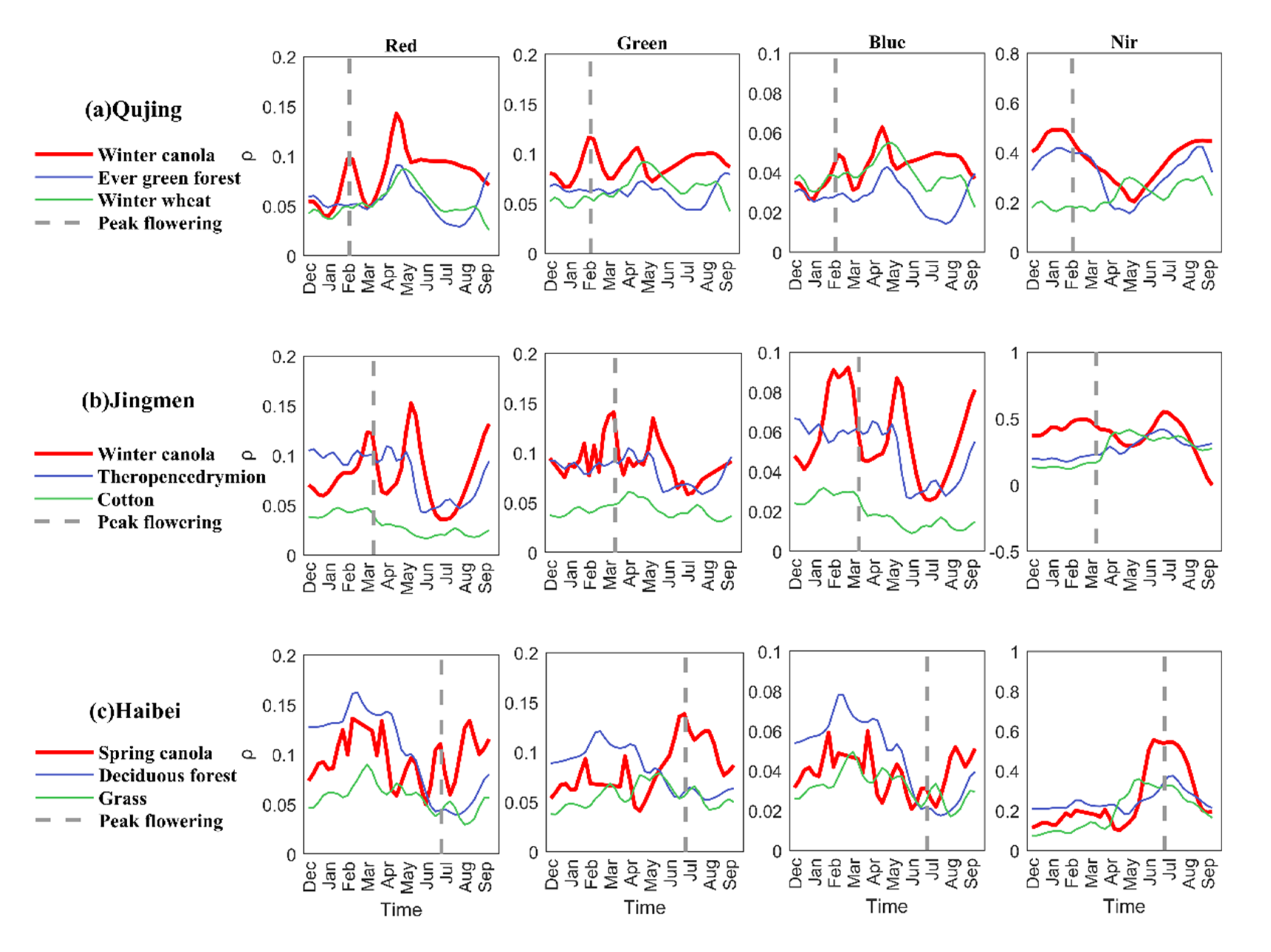
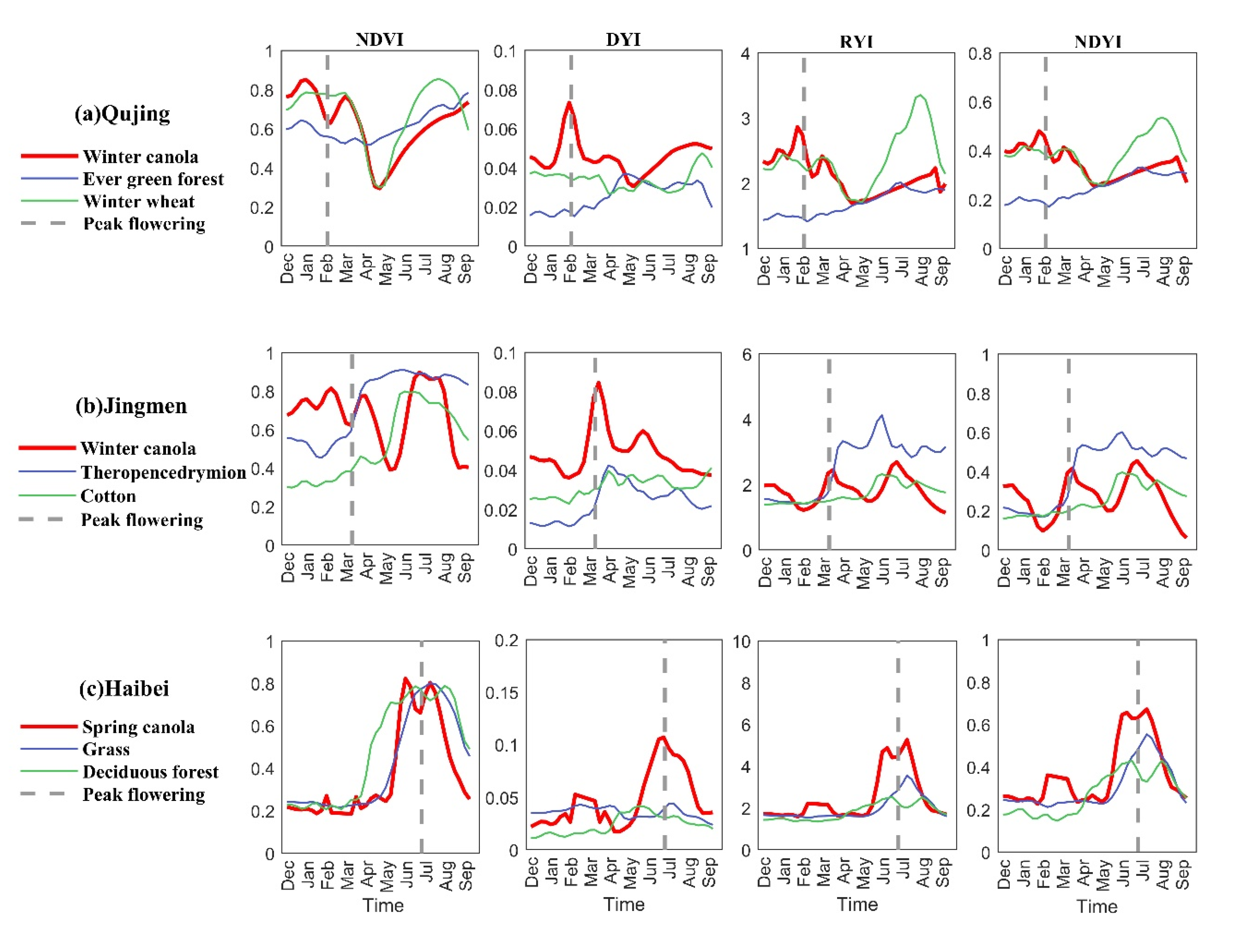
2.3. Temporal Characteristics of Canola Spectra

Several spectral time-series samples from three sites (Qujing, Jingmen, and Haibei) were selected to investigate the temporal characteristics of spectral reflectance for different vegetation types. Canola in different sites showed consistent local peaks in the red and green bands during flowering (Figure 3). In particular, the green reflectance of canola flowers is much higher than that of other vegetation types. In contrast, all the vegetation, including canola, showed similar low reflectance in the blue band. Thus, in the previous yellowness indices, the green and blue bands are commonly used as measured and reference bands, respectively.
Figure 4 further compares the time-series of different yellowness indices, including RYI, NDYI, and DYI. All three indices showed peaks during the flowering period. However, RYI and NDYI of winter canola in Qujing and Jingmen were not much higher than those of other vegetation types; indeed, there was a small valley during flowering for spring canola in Haibei. This may be because the ratio-formed indices are sensitive to noise in the denominator, especially because the blue band is influenced by atmospheric effects. In contrast, DYI of canola in all three regions showed a clear peak during flowering, and the peak values were much higher than those of other vegetation types. Thus, DYI was selected in this study for capturing the yellowness signal. NDVI time-series were also compared because the yellow flower can reduce the NDVI [9]. The NDVI of canola increases before flowering and then declines when canola starts flowering. After canola flowers start to senesce, NDVI increases again, and then declines when canola starts maturing. Thus, these two local maximum points of NDVI time-series valley are distinctive features that can be used to identify the duration of flowering. In contrast, the peak of DYI time-series does not necessarily match with the period of flowering. For example, DYI time-series of canola in Haibei continued to increase with increased greenness before flowering. Thus, the NDVI time-series was employed in this study to determine the period of flowering, as supplementary information to green and blue bands.

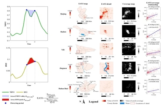
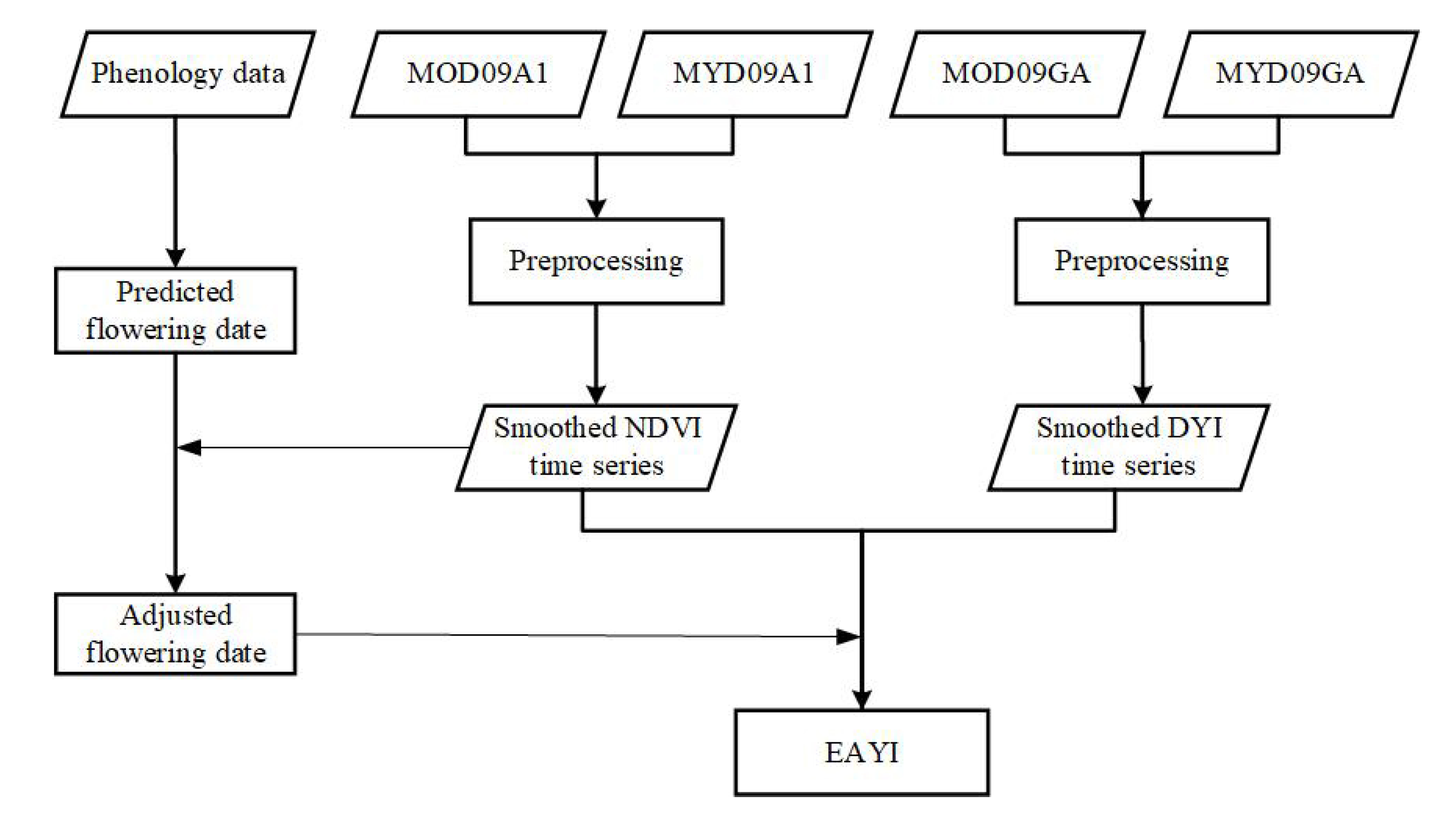
2.4. Development of the EAYI for Canola Flowering Mapping

The EAYI was developed to detect canola flowers in five subregions. The main steps of the calculation of the EAYI are shown in Figure 5. First, phenological data obtained from agrometeorological stations were used to roughly predict the flowering date of canola across China. Second, smoothed NDVI time-series were generated from MOD09A1 and MYD09A1 data, and smoothed DYI time-series were generated from MOD09GA and MYD09GA data. Third, the precise flowering period was further estimated by adjusting the initial predicted flowering date with the NDVI time-series. Finally, the EAYI was calculated using the DYI peak and NDVI valley during the estimated period of flowering.

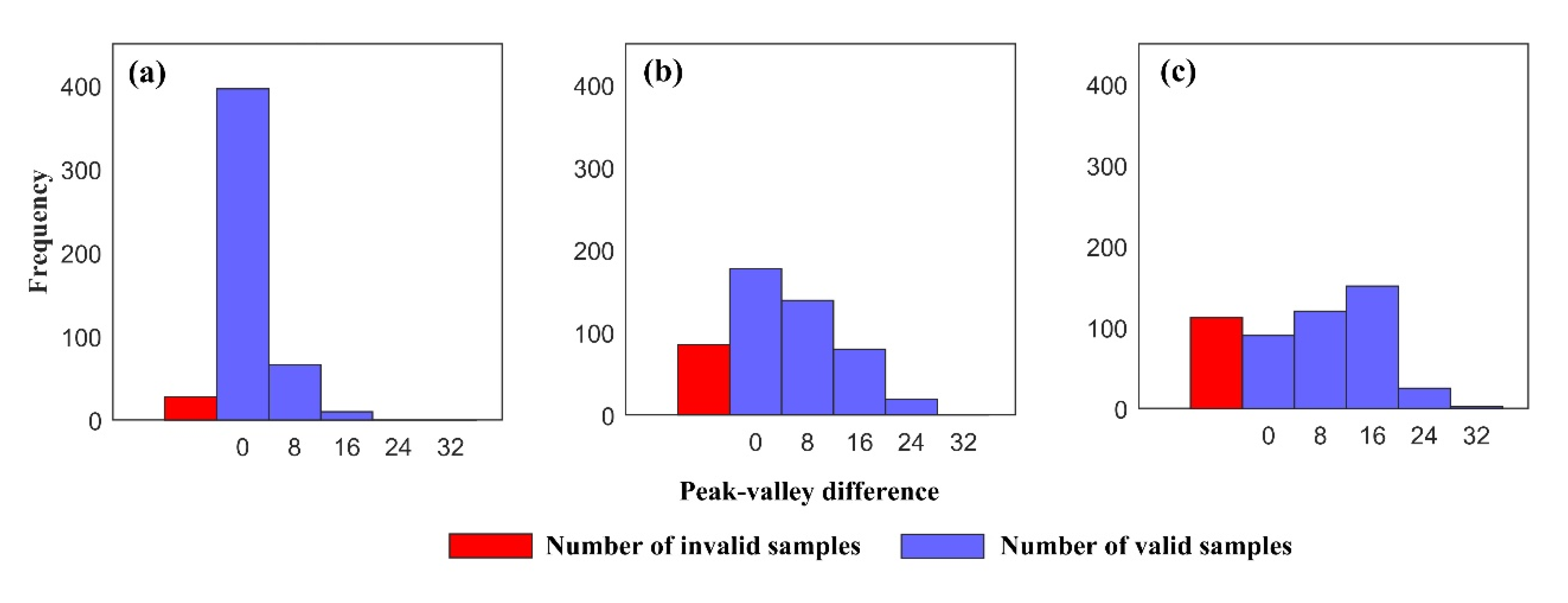
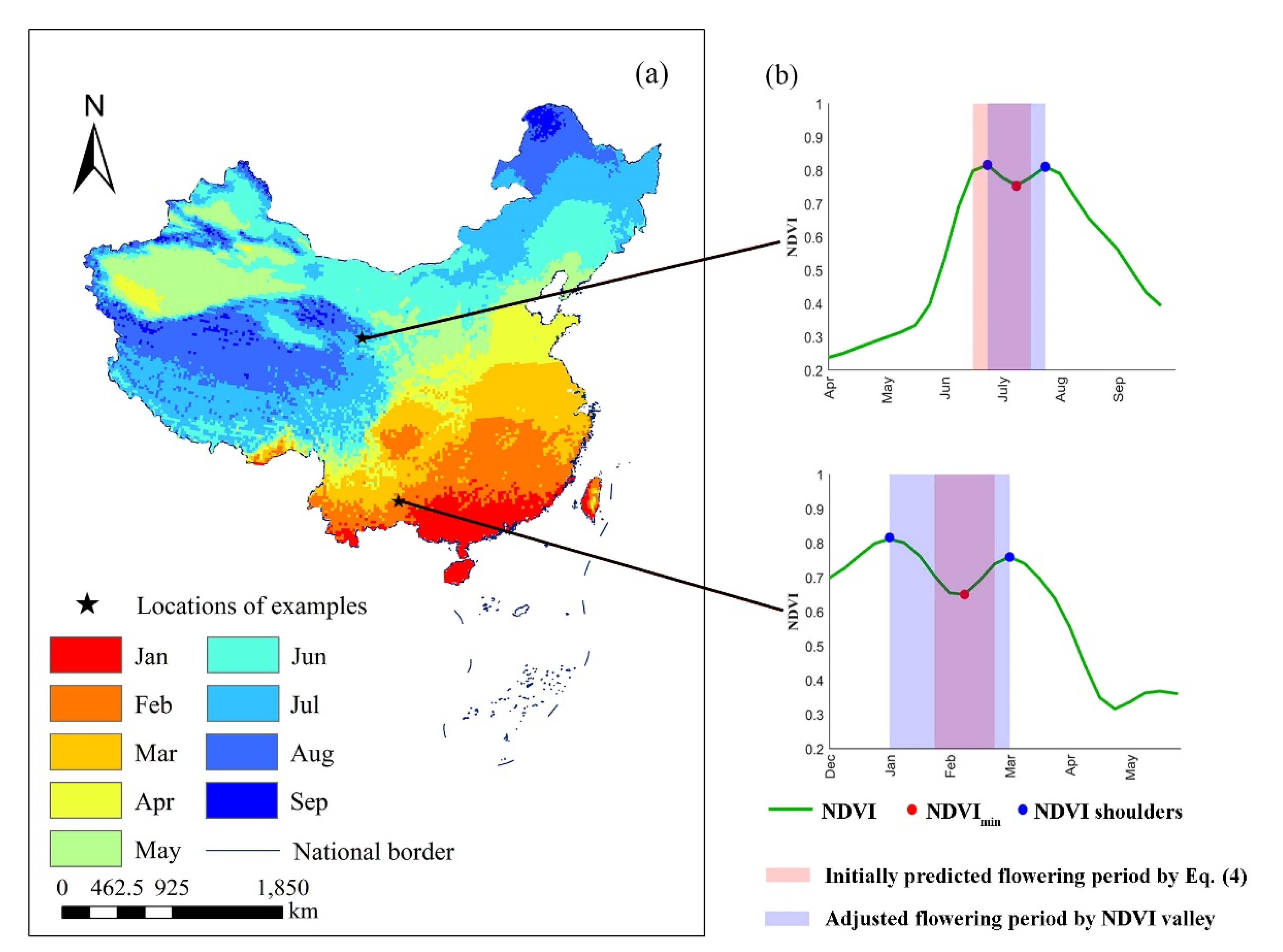
2.4.1. Determination of the Flowering Period

Determination of the flowering period is vital for capturing the yellow signal of canola flowers. As the flowering period is primarily related to location, a linear regression model was employed here to predict the preliminarily the flowering date (T) using latitude (Lat), longitude (Lon), and altitude (Alt) as follows:
T   =   a Lat   +   b Lon   +   c Alt   +   d ,
where the a, b, c, and d are the regression coefficients of latitude, longitude, altitude, and constant. Taking the multi-year average peak flowering date recorded by the agrometeorological stations as the dependent variable, and the corresponding longitude, latitude, and altitude as the explained variables, the a, b, c, and d were determined as 7.07, 1.508, 0.03, −318.11 respectively. The R2 of this regression model achieves 0.90, indicating that such an empirical model can estimate the peak flowering date with reasonable accuracy. Then, the peak flowering date across China was initially predicted using Equation (4). In general, the initially predicted flowering date becomes later from southern to northern areas, and from low-altitude to high-altitude areas (Figure 6a). Because the peak flowering date varies year on year due to climate variation, the actual date of peak flowering could vary by month (T − 16, T + 16). Thus, the precise flowering period was further adjusted by the valley of the NDVI time-series. Specifically, if there was a local minimum NDVI value in the period T − 16 to T + 16 for a pixel, this pixel was considered to be a potential canola pixel. The two local maximum points of the NDVI time-series valley were then considered as the beginning and end of the flowering period (Figure 6b).

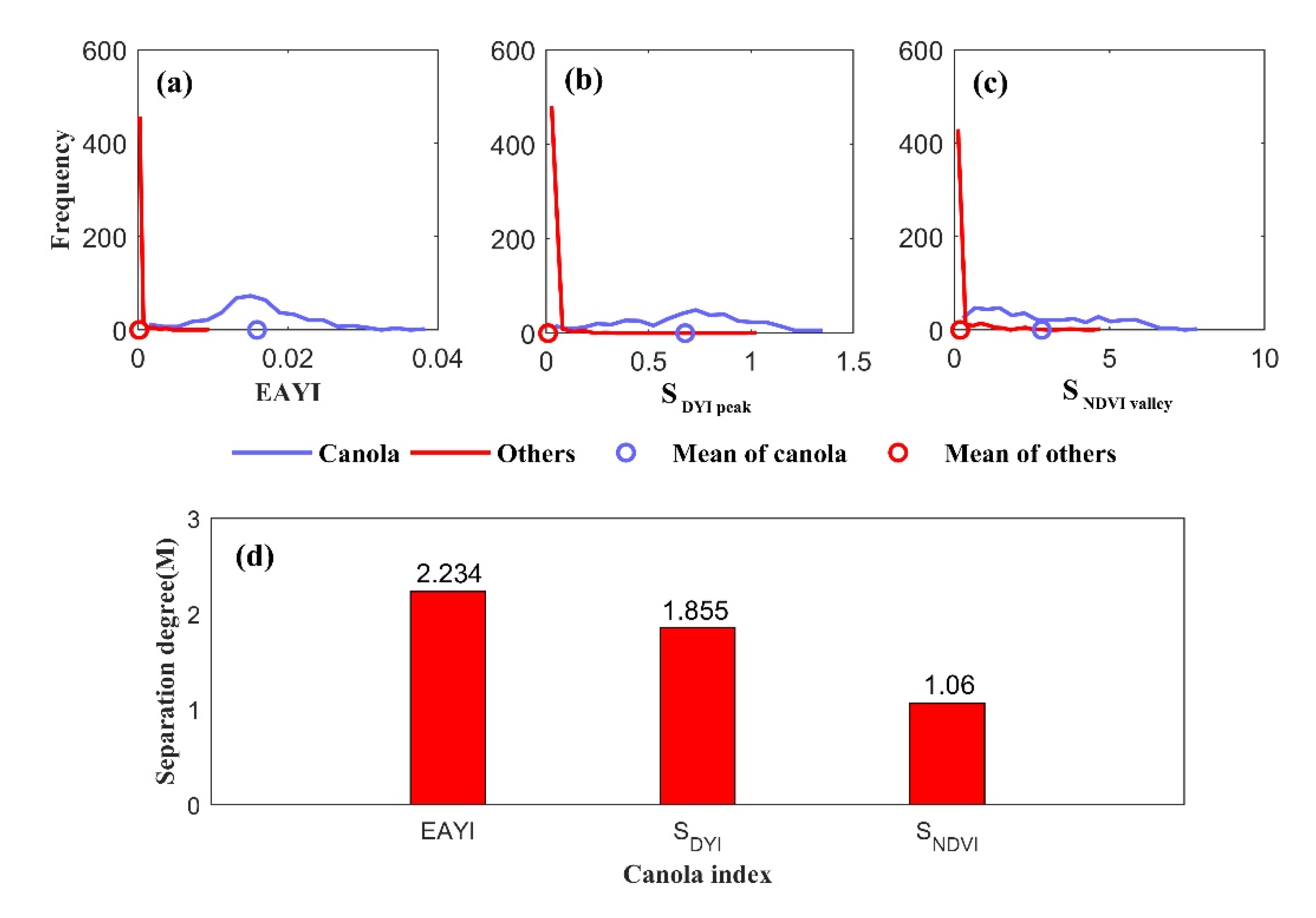
2.4.2. EAYI Index for Canola Flowering Mapping

The EAYI was developed by combining the peak of DYI time-series and the valley of NDVI time-series during the flowering period as follows:
EAYI   =   S DYI   peak   t 2     t 1 1     S NDVI   valley   t 2     t 1 = t 1 t 2 ( DYI t     0.5   ( DYI t 1   +   DYI t 2 ) ) ( t 2     t 1 )     t 1 t 2 ( 0.5 ( NDVI t 1   +   NDVI t 2 )     NDVI t ) ,
where S DYI   peak and   S NDVI   valley are areas of DYI time-series peak and NDVI time-series valley during the flowering period, and t1 and t2 are the beginning and end dates of the estimated flowering period (Figure 7). The term (t2 − t1) was used to normalize the areas of DYI time-series peak and NDVI time-series valley, because the length of the flowering period varies from site-to-site. A higher EAYI corresponds to a higher density of canola flowers.
Two constraints were added to directly exclude non-canola pixels. First, a pixel was excluded if there was no valley in NDVI time-series during the predicted flowering period, in other words, the minimum value of NDVI appears at the edge of the estimated flowering period because the valley of the NDVI time-series is a key feature to identify a canola pixel. Second, a pixel was also excluded if the local minimum value of the NDVI valley in the flowering period was less than 0.5 because canola is in a green state during the period of flowering.

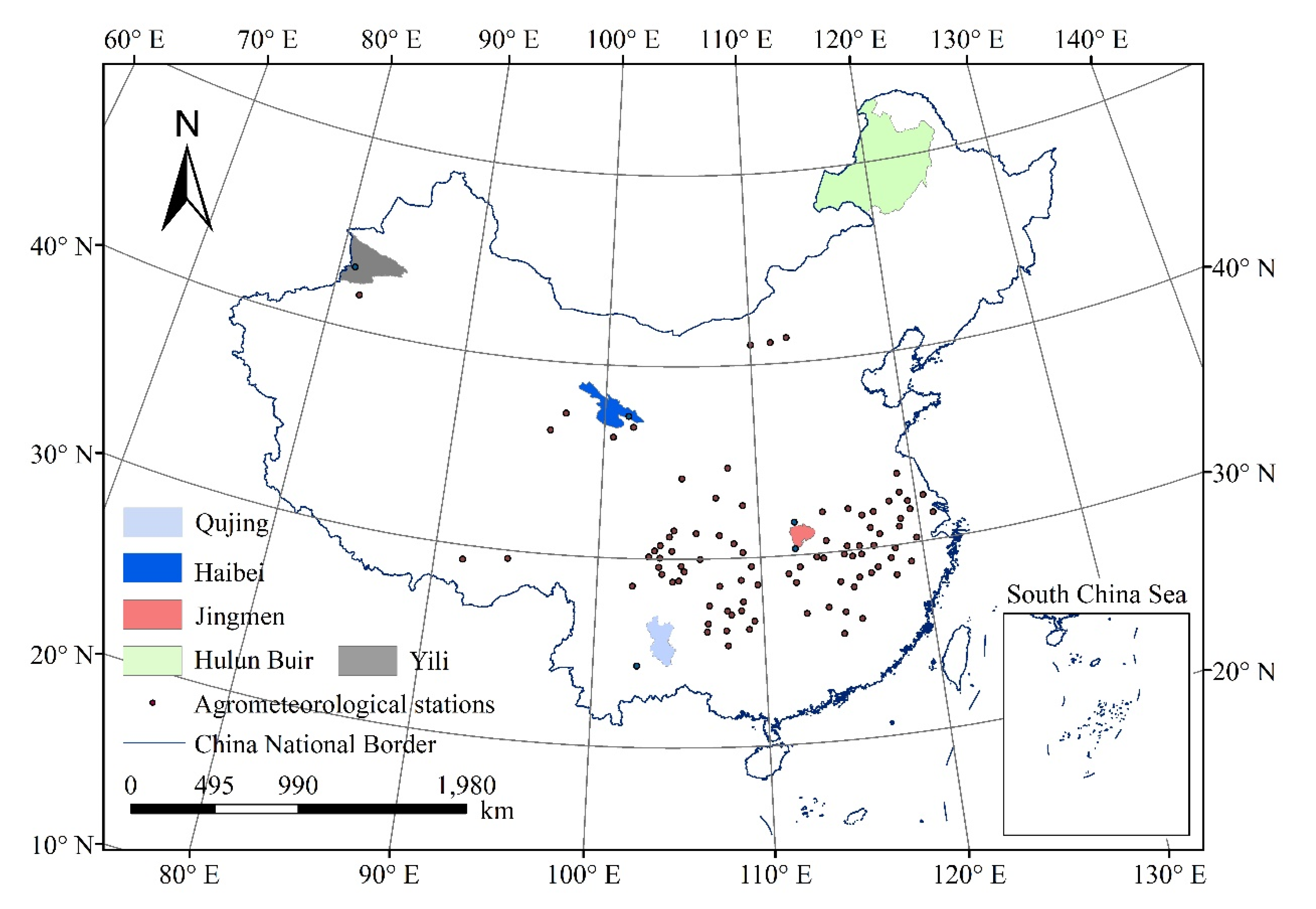
2.5. Mapping and Evaluation of the EAYI

The EAYI in five research areas was calculated from MODIS data from 2003 to 2017. Canola coverage, interpreted from high-resolution images acquired in 2017, was used to evaluate the spatial mapping results of the EAYI. For each study area, 500 samples of canola coverage were randomly selected for comparison, except that only 35 pixels were selected in Hulun Buir because of the low canola density and serious cloud contamination in the high-resolution image.
Because the canola flower is a key indicator of seed yield, the census canola yield of Qujing, Haibei, Jingmen, and Hulun Buir from 2003 to 2017 was used for validating temporal variation of the EAYI, whereas the census yield of Yili from 2006 to 2017 was used for validation due to the lack of census data before 2006 in Yili. In the long-term analysis of crop yield, the actual crop yield (Y) is generally decomposed into three parts [17,18,19]: trend yield (τ), meteorological yield (W), and random error (ε) as follows:
Y =   τ   +   W   +   ε ,
The trend yield is a long-period yield component which varies with the improvement of crop varieties, harvesting techniques and statistical methods, which is also called technical yield. Meteorological yield is a fluctuating yield component that is affected by short-period change factors dominated by climate elements. As the harvesting techniques and statistical methods are not related with the flower amount, the meteorological yield that removes the trend yield might be better related with flower amount and proposed EAYI index. Thus, the meteorological yield was also calculated for comparison. A commonly used method, the Hodrick–Prescott (HP) filter [20], was used to separate the meteorological yield from the trend yield. Given a suitable positive number λ, the trend yield was defined as satisfying Equation (7):
min ( t = 1 T ( Y t τ t ) 2 + λ t = 2 T 1 [ ( τ t + 1 τ t ) ( τ t τ t 1 ) ] 2 ) ,
where λ controls variation of the trend. The larger the λ, the greater the variation of the trend. λ was set as 100, according to previous studies [21]. Meteorological yield was then calculated as:
W   =   Y     τ ,
The estimated meteorological yield was used to validate temporal variation of the total EAYI in each study area.
For comparison, three canola indices proposed in previous studies, RYI [6], NDYI [7], and a canola index proposed by Ashourloo et al. [5] (denoted as Ashourloo CI hereafter) were also calculated from MOD09GA and MYD09GA time-series. The Ashourloo CI is calculated as:
Ashourloo   CI = B 2 ( B 1 + B 4 ) ,
where B1, B2, and B4 are the red, near infrared, and green bands of the MODIS instrument, respectively. As the previous canola indices were originally calculated from a specific image scene captured in the flowering period, they cannot be directly calculated from MODIS time-series. Thus, a similar composition procedure of DYI was conducted. Specifically, the RYI, NDYI, and Ashourloo CI time-series were firstly composited, with an eight-day maximum composing criterion. Then, the canola indices images of the peak flowering date determined by the valley of NDVI time-series were selected to map canola flowers.

3. Results

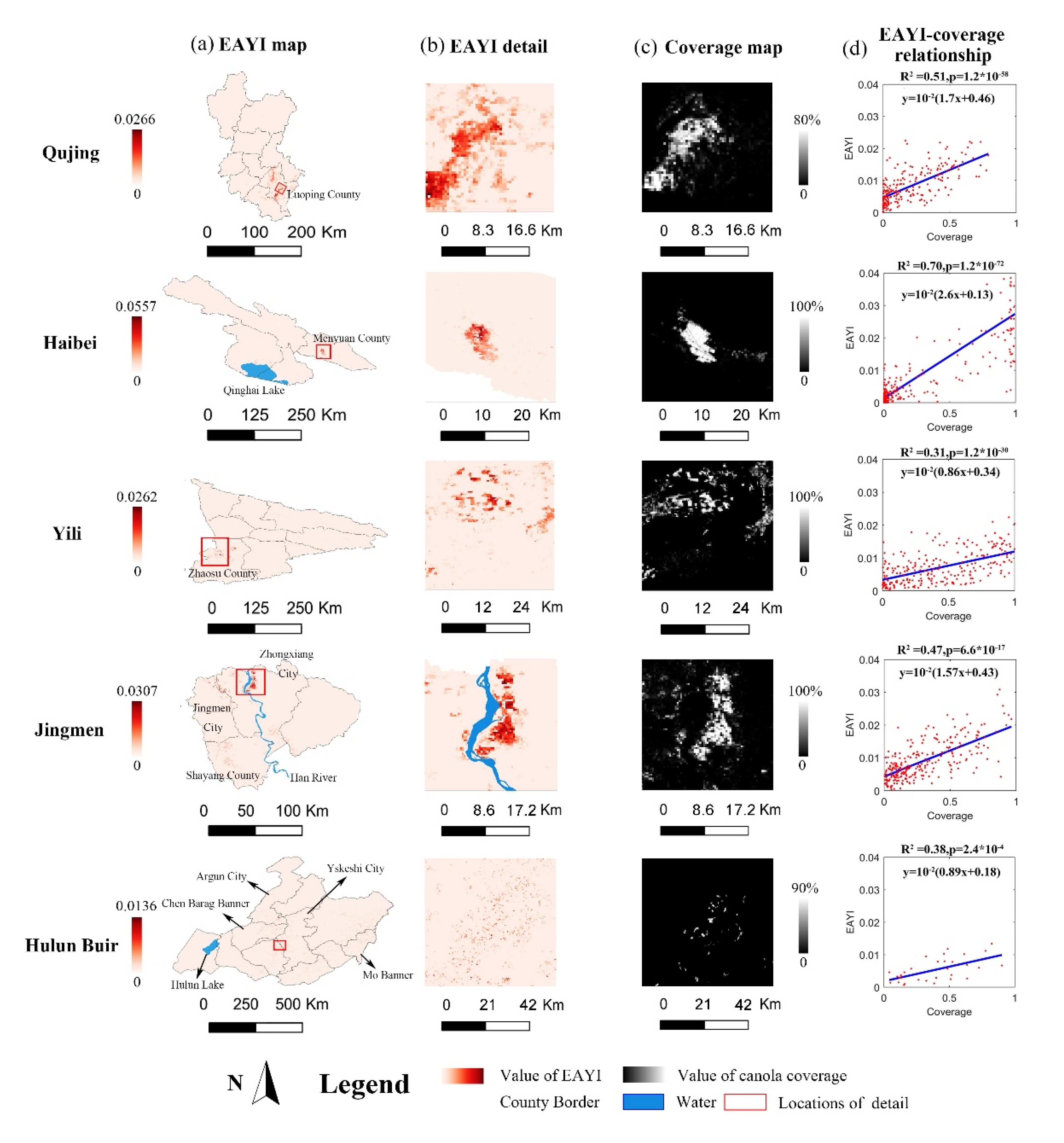
3.1. EAYI Map Derived from MODIS Data

The EAYI maps of five areas during 2003–2017 were generated from MODIS data (Figure 8). For Qujing, canola was mainly planted in Luoping County, consistent with a previous study [22]. Canola in Haibei was mainly planted in Menyuan County and northeast of Qinghai Lake, which has become a famous tourist landscape in Qinghai [23]. Canola in Yili was mainly planted in Zhaosu County (west of Yili), which was the main canola production area in the Xinjiang Uygur Autonomous Region [24]. Canola in Jingmen was widely planted across the whole prefecture, including Zhongxiang City, Jingmen City, and Shayang County, similar to previous studies [11]. Canola in Hulun Buir was relatively sparse, mainly planted in the junction of Yakeshi City, Argun City, Chen Barag Banner, and west of Mo Banner, consistent with a previous study [25] showing a main canola planting in Yakeshi City and Argun City.

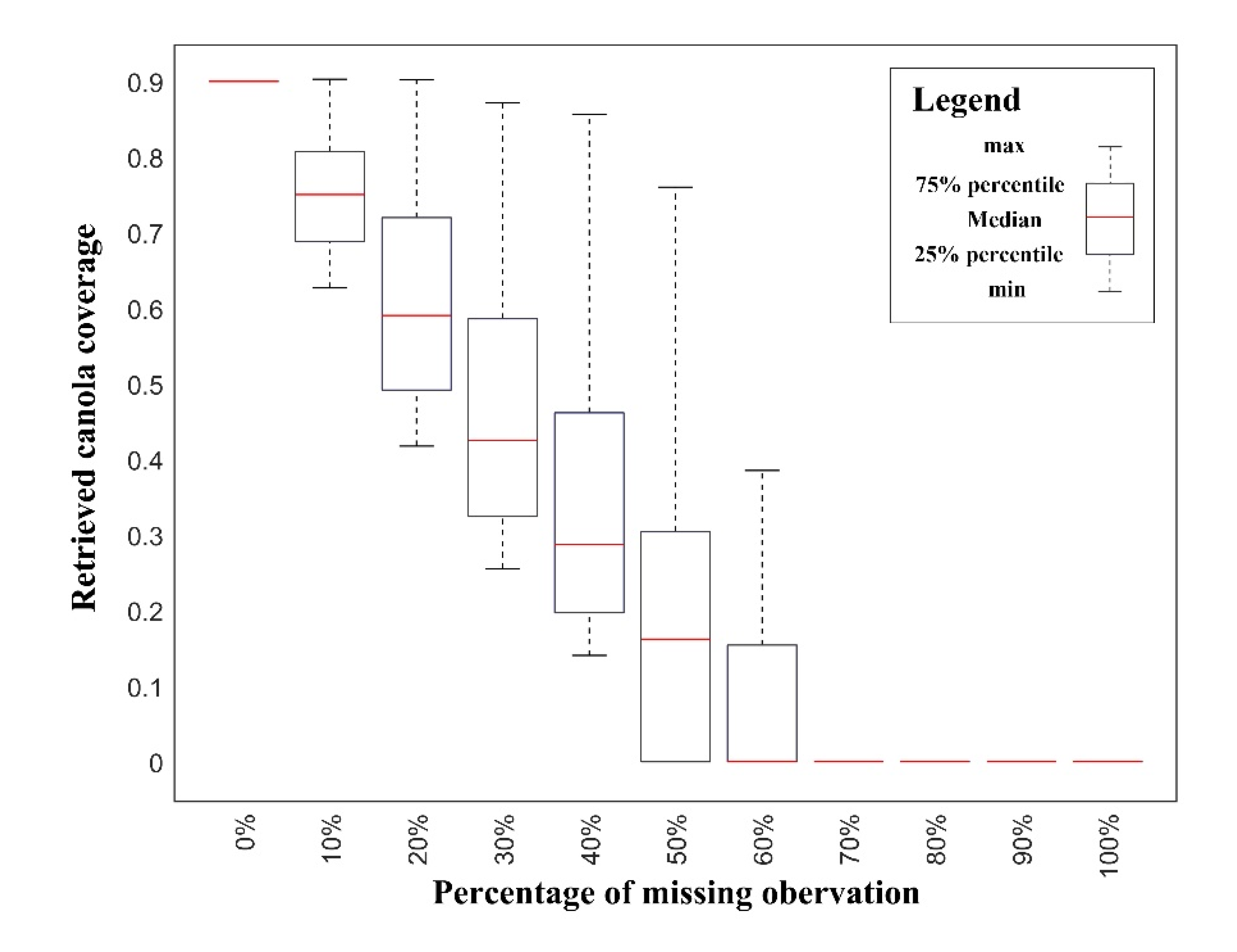
3.2. Comparison with Canola Coverage Interpreted from High-Resolution Imagery

The EAYI maps show a good consistent spatial pattern with the reference canola coverage map derived from high-resolution images (Figure 8b,c). In contrast, the maps of three previous canola indices match the reference maps relatively worse (Figure S1). Figure 8d further shows the relationship between the EAYI and reference canola coverage. There are significant correlations between the EAYI and canola coverage in all five study areas with R2 ranged from 0.31 to 0.70. In contrast, the correlation between previous canola indices and coverage are relatively lower with R2 ranged from 0.02 to 0.43 (Figure S2). This indicates that EAYI is a better indicator of the density of canola flowers. However, the regression coefficients vary across sites. The regression slope was relatively small for areas with dispersed-planted canola, including Yili and Hulun Buir. The results imply that the sensitivity of the EAYI is not consistent across different areas.

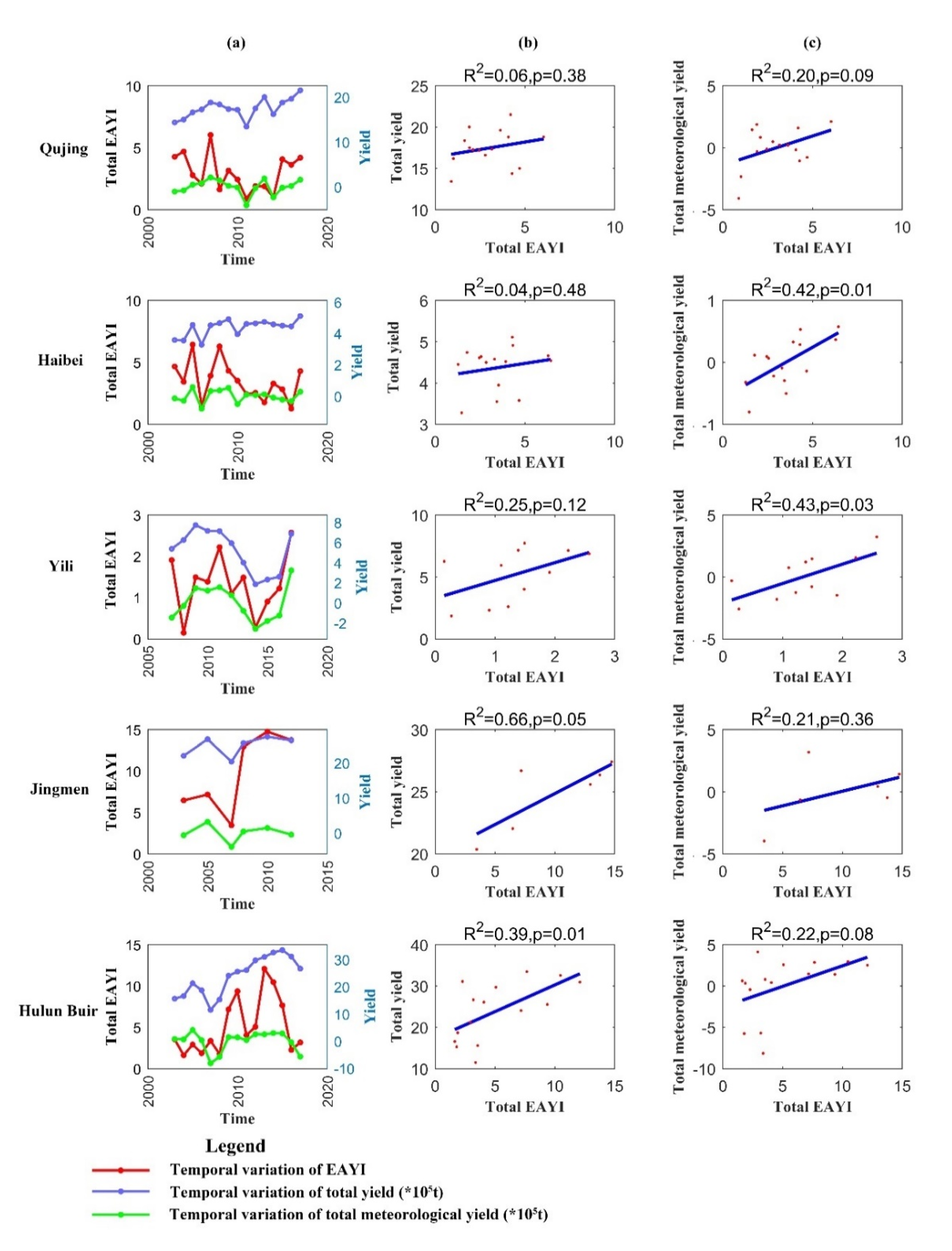
3.3. Comparison with Census Yield Data

The multi-year total EAYI from 2003 to 2017 was calculated and compared with census yield data in five areas (Qujing, Haibei, Yili, Jingmen, and Hulun Buir). The total EAYI in Jingmen was calculated only in 2003, 2005, 2007, 2008, 2010, and 2012 due to heavy cloud contamination. The temporal change in the EAYI was consistent with the temporal variation of census yield in Yili, Jingmen, and Hulun Buir, whereas the consistencies in Qujing and Haibei were poor (Figure 9b). However, temporal changes in the EAYI were somewhat consistent with short-term fluctuation of census yield in all five subareas (Figure 9a). Thus, multi-year EAYI values were further compared with meteorological yield, which reflects short-term variation in actual yield. There were positive correlations between meteorological yield and total EAYI in all five subareas (Figure 9c), although the correlation was not necessarily significant due to small sample sizes. These results indicate that the EAYI could be a potential indicator of short-term changes in yield. In contrast, the previous canola indices poorly indicate the total yield and meteorological yield with very low correlation or even negative correlation between the indices and yield (Figures S3–S5).

4. Discussion

4.1. Superiorities of the EAYI

The first improvement of this study was the estimation of the flowering before the calculation of the EAYI. Estimation of the flowering period is particularly important for canola mapping over China due to the large variation in the timing of flowering across different areas. Thus, a method of estimating the period of flowering, combining an empirical regression model and NDVI time-series, was undertaken in this study. The multi-year date of peak flowering observed at five agrometeorological stations in the study areas (Figure 10a) were used to validate the period of flowering estimated by our proposed method. The period of flowering estimated in the present study encompassed the observed dates of peak flowering across all five stations (Figure 10b–f). Moreover, temporal changes in the NDVI valley dates were also consistent with those of the observed dates of peak flowering although there was some inconsistency in No.56875 station and No.51437 station. Such inconsistency might be partly induced by the inconsistent standards of field phenological observation at different sites and different periods [26,27,28]. However, such uncertainty in the estimation of peak flowering date will not largely affect the calculation of EAYI, because the EAYI is calculated based on the area of DYI peak and NDVI valley during the whole flowering period that may keep one to two months. In general, the NDVI time-series was an important data source for detecting flowering, and the flowering periods estimated by our method can correctly estimate the actual periods of flowering.
The use of DYI instead of RYI or NDYI is another point of difference in this study compared to previous studies [5,6,7]. Our experiment shows that the EAYI has a better agreement with reference to canola spatial distribution and the temporal variation of census yield compared with previous indices. Indeed, the detected yellowness peak should match the NDVI valley for canola pixels if the yellowness index robustly detected yellow flowers. To confirm this, 500 canola samples with a minimum coverage of 50%, in five study areas, were selected to investigate the time difference between the yellow indices peak and the NDVI valley. The DYI peak exhibited the best consistency with the NDVI valley, with a time difference of less than 8 days (Figure 11). In contrast, the peaks of RYI and NDYI were poorly consistent with the NDVI valley. This confirmed that DYI was a more suitable index, reflecting the yellow signal peak in the MODIS time-series. The better performance of DYI in capturing yellowness signals might be attributed to its relative resistance to the atmospheric effect, which consists of the extinction effect and path radiance. For short-wavelengths, including the blue and green bands, path radiance accounts for a larger proportion of the atmospheric effect, which means that the apparent reflectance can be written as:
R TOA = R surface + R path ,
where R TOA , R surface and R path are top of atmosphere radiance, surface radiance and path radiance respectively. The common path radiance for blue and green bands could be effectively eliminated by subtraction. In contrast, the use of a ratio allows better performance in eliminating the extinction effect, rather than the path radiance. Thus, DYI performed better than the ratio-based indices (RYI and NDYI) in this study. Ratios are often used in vegetation indices because they employ near-infrared and red bands that have longer wavelengths, where the extinction effect cannot be ignored.
Finally, the EAYI combines the DYI peak and the NDVI valley to enhance the yellowness signal. To confirm the effectiveness of such an enhancement, we further compared the separation degree of EAYI, area of the DYI peak, and area of the NDVI valley among different canola pixels and other land-cover pixels. Five hundred canola samples, with a coverage exceeding 50%, and 500 other land-cover samples from five study areas, were selected randomly to calculate the separation degree defined by Equation (11) [29,30] for three indices:
M = | μ 1 μ 2 | σ 1 + σ 2 ,
where μ 1 and μ 2 are the mean values of canola samples and other land-cover type samples, respectively; | μ 1 μ 2 | denotes the interclass variability; σ 1   and σ 2 are the standard deviations of canola samples and other land-cover type samples. A higher M indicates better separation of the two types of samples. The EAYI values of canola and other land-cover samples have the most distinctive distributions and the highest degree of separation, followed by the area of the DYI peak and the area of the NDVI valley (Figure 12). These results confirmed the effectiveness of the EAYI in distinguishing canola flowers from other land-cover types.
In summary, the proposed EAYI index can be used for detecting canola flowers across a large area if field observed phenological data is available to establish an empirical regression model for predicting the peak flowering date roughly. Moreover, a combination of NDVI valley and DYI peak enhances the yellowness signal in mixed pixels, thus EAYI is applicable for coarse-resolution data like the MODIS time-series which is available in a long-term period.

4.2. Remaining Challenges and Future Researches

Cloud contamination is a serious issue for flower detection because canola often flowers in the rainy season. Here, a simulation experiment was conducted to explore the sensitivity of the proposed EAYI to a number of invalid observations. First, typical NDVI and DYI time-series of canola were calculated from 100 high-coverage canola pixels (>90%) in Jingmen; 10–100% of the observations were then randomly removed from the flowering period. Finally, coverage was retrieved by the Jingmen fitting equation (Figure 8d). The EAYI was very sensitive to missing observations (Figure 13). The retrieved coverage decreased to 0.4 when there were 30% invalid observations, and it further decreased to 0 when missing observations accounted for more than 60% of the total. Thus, frequent observations are needed to detect canola flowers. In this study, the daily observations available through MODIS generally satisfied this requirement. However, the availability of frequent satellite observations at higher resolutions is still limited, indicating a challenge in mapping canola at higher spatial resolutions. Spatial-temporal fusion techniques [31,32] might be helpful in addressing this issue.
Another limitation of the EAYI is the varying sensitivity to canola coverage in different regions (Figure 8d), which raises the difficulty in retrieving the coverage or determining a uniform threshold for canola mapping in different regions. Finally, the EAYI remains a poor indicator of actual canola yield for some study areas, although this study demonstrated a correlation between multi-year EAYI values and the meteorological yields in most regions. This implies a complex relationship between actual yield and the quantity of canola flowers or the EAYI. Thus, the role of the EAYI in monitoring canola yield requires further exploration and validation in the future.
Due to the above limitations, automatically mapping canola flowers over the whole of China is still challenging, especially in the cloudy areas and the fragmented areas. Thus, a portrait of canola flower distribution over China is still missing at this stage. In next step, we will attempt to detect canola flower signals by combing more data sources, e.g., multi-resolution optical data and synthetic aperture radar (SAR) data, with advanced fusion techniques [32,33]. Moreover, more field data is planned for collection to explore the relationship between canola yield and flower amount.

5. Conclusions

In this study, a new canola index, EAYI, was proposed for canola mapping in regions across a wide range of longitudes and latitudes, using the NDVI and DYI time-series derived from MODIS data. A method for estimating flowering was employed to overcome the problems of differences in the timing of flowering over large areas. The EAYI, which achieved an enhancement of the weak yellow signal in coarse pixels, was shown to be effective in canola mapping with MODIS data. Validation using the reference maps and census data demonstrated that the EAYI is a potential index for mapping canola flowers over a large area and tracing the changes in a long-term period.

Supplementary Materials

The following are available online at https://www.mdpi.com/2072-4292/12/23/3912/s1, Figure S1. (a) Canola coverage map derived from high-resolution imagery in five subareas. Comparisons of the (b) EAYI maps, (c) RYI maps, (d) NDYI maps, (e) Ashourloo CI maps, Figure S2. Comparisons of the relationship between four canola indices (a) EAYI, (b) RYI, (c) NDYI, (d) Ashourloo CI and coverage derived from high-resolution imagery in five subareas, Figure S3. (a) The temporal variation of total RYI, total yield and total meteorological yield in five subareas; (b) The relationship between total RYI and total yield in five subareas; (c) The relationship between total RYI and meteorological yield in five subareas, Figure S4. (a) The temporal variation of total NDYI, total yield and total meteorological yield in five subareas; (b) The relationship between total NDYI and total yield in five subareas; (c) The relationship of total NDYI and meteorological yield in five subareas, Figure S5. (a) The temporal variation of total Ashourloo CI, total yield and total meteorological yield in five subareas; (b) The relationship between total Ashourloo CI and total yield in five subareas; (c) The relationship of total Ashourloo CI and meteorological yield in five subareas.

Author Contributions

Conceptualization, X.C. (Xuehong Chen), J.C., and Y.Z.; Methodology, Y.Z., X.C., (Xuehong Chen) and Y.T.; Validation, Y.Z.; Formal Analysis, Y.Z.; Resources, X.C. (Xuehong Chen), X.C. (Xin Cao), Y.S., and X.C. (Xihong Cui); Writing—Original Draft Preparation, Y.Z. and X.C. (Xuehong Chen); Writing—Review and Editing, J.C., Y.T., Y.S., and X.C. (Xihong Cui); Funding Acquisition, X.C. (Xuehong Chen). All authors have read and agreed to the published version of the manuscript.

Funding

This work was funded by National Natural Science Foundation of China (No. 41871224).

Conflicts of Interest

The authors declare no conflict of interest.

References

  1. Zhang, X.; He, Y. Rapid estimation of seed yield using hyperspectral images of oilseed rape leaves. Ind. Crop. Prod. 2013, 42, 416–420. [Google Scholar] [CrossRef]
  2. Li, L. Research on Farmers’ Landscape Rape Planting Behavior in Huhai Tourism Destination; Jiangxi Agricultural University: Nanchang, China, 2016. [Google Scholar]
  3. Yin, Y.; Wang, H. Current situation and Development Trend of Rapeseed production in China. Agric. Outlook 2011, 7, 43–45. [Google Scholar]
  4. Liu, C.; Feng, Z.; Xiao, T. Development status, potential and countermeasures of Rape industry in China. Chin. J. Oil Crop. 2019, 41, 485. [Google Scholar]
  5. Ashourloo, D.; Shahrabi, H.S.; Azadbakht, M.; Aghighi, H.; Nematollahi, H.; Alimohammadi, A.; Matkan, A.A. Automatic canola mapping using time series of sentinel 2 images. Isprs J. Photogramm. Remote Sens. 2019, 156, 63–76. [Google Scholar] [CrossRef]
  6. Sulik, J.J.; Long, D.S. Spectral indices for yellow canola flowers. Int. J. Remote Sens. 2015, 36, 2751–2765. [Google Scholar] [CrossRef]
  7. Sulik, J.J.; Long, D.S. Spectral considerations for modeling yield of canola. Remote Sens. Environ. 2016, 184, 161–174. [Google Scholar] [CrossRef] [Green Version]
  8. Fang, S.; Tang, W.; Peng, Y.; Gong, Y.; Dai, C.; Chai, R.; Liu, K. Remote estimation of vegetation fraction and flower fraction in oilseed rape with unmanned aerial vehicle data. Remote Sens. 2016, 8, 416. [Google Scholar] [CrossRef] [Green Version]
  9. Shen, M.; Chen, J.; Zhu, X.; Tang, Y. Yellow flowers can decrease NDVI and EVI values: Evidence from a field experiment in an alpine meadow. Can. J. Remote Sens. 2009, 35, 99–106. [Google Scholar] [CrossRef]
  10. Shen, M.; Chen, J.; Zhu, X.; Tang, Y.; Chen, X. Do flowers affect biomass estimate accuracy from NDVI and EVI? Int. J. Remote Sens. 2010, 31, 2139–2149. [Google Scholar] [CrossRef]
  11. Tao, J.; Wu, W.; Liu, W.; Xu, M. Exploring the Spatio-Temporal Dynamics of Winter Rape on the Middle Reaches of Yangtze River Valley Using Time-Series MODIS Data. Sustainability 2020, 12, 466. [Google Scholar] [CrossRef] [Green Version]
  12. d’Andrimont, R.; Taymans, M.; Lemoine, G.; Ceglar, A.; Yordanov, M.; van der Velde, M. Detecting flowering phenology in oil seed rape parcels with Sentinel-1 and-2 time series. Remote Sens. Environ. 2020, 239, 111660. [Google Scholar] [CrossRef] [PubMed]
  13. Tao, J.; Wu, W.; Xu, M. Using the Bayesian Network to map large-scale cropping intensity by fusing multi-source data. Remote Sens. 2019, 11, 168. [Google Scholar] [CrossRef] [Green Version]
  14. Mercier, A.; Betbeder, J.; Baudry, J.; Le Roux, V.; Spicher, F.; Lacoux, J.; Roger, D.; Hubert-Moy, L. Evaluation of Sentinel-1 & 2 time series for predicting wheat and rapeseed phenological stages. ISPRS J. Photogramm. Remote Sens. 2020, 163, 231–256. [Google Scholar]
  15. Lei, Y. Development status and Countermeasures of rape industrialization in Luoping County. Yunnan Agric. Sci. Technol. 2003, 6, 1–2. [Google Scholar]
  16. Chen, J.; Jönsson, P.; Tamura, M.; Gu, Z.; Matsushita, B.; Eklundh, L. A simple method for reconstructing a high-quality NDVI time-series data set based on the Savitzky–Golay filter. Remote Sens. Environ. 2004, 91, 332–344. [Google Scholar] [CrossRef]
  17. Fang, S. Separation of trend yield and climate yield. Chin. J. Nat. Disasters 2011, 20, 13. [Google Scholar]
  18. Wadleigh, C.H.; Shaw, R.H.; Thompson, L.M.; Dale, R.F.; Auer, L.; Durost, D.D.; Hurst, R.L.; Willett, H.C.; Bean, L.H.; Palmer, W.C.; et al. Weather and Our Food Supply; Center for Agricultural and Economic Development, Iowa State University: Ames, IA, USA, 1964; pp. 9–22. [Google Scholar]
  19. Zhang, J.; Zhao, Y.; Ding, Z. Research on the relationships between rainfall and meteorological yield in irrigation district. Water Resour. Manag. 2014, 28, 1689–1702. [Google Scholar] [CrossRef]
  20. Hodrick, R.J.; Prescott, E.C. Postwar US business cycles: An empirical investigation. J. Money Credit Bank 1997, 1–16. [Google Scholar] [CrossRef]
  21. Wang, G.Z.; Lu, J.S.; Chen, K.Y.; Wu, X.H. Exploration of method in separating climatic output based on HP filter. Chin. J. Agrometeorol. 2014, 35, 195–199. [Google Scholar]
  22. Li, J.; Liu, C.; Wang, H.; Zhang, J. Study on extraction Method of Planting area of Rapeseed from Luoping based on multi-source remote sensing data. J. Southwest. Univ. (Nat. Sci.) 2008, 38, 33–138. [Google Scholar]
  23. He, Y.; Min, X.; Jiang, G.; Jian, X.; Gao, Q.; She, S. On the Characteristics and Enlightenment of rapeseed flower Tourism Development around Qinghai Lake under eye Effect. Hunan Agric. Sci. 2016, 11, 76–78. [Google Scholar]
  24. Cui, H.; Yao, Q.; Chen, J.; Lin, X. Current situation and development ideas of spring rapeseed production in Zhaosu region. Anhui Agric. Sci. Bull. 2016, 22, 38–40. [Google Scholar]
  25. Lian, B.; Guo, J.; Jiao, Y. Discussion on the current situation, Problems and Countermeasures of rape industry development in Hulun Buir city. Inn. Mong. Agric. Sci. Technol. 2010, 3, 76–77. [Google Scholar]
  26. Chen, X.; Wang, W.; Chen, J.; Zhu, X.; Shen, M.; Gan, L.; Cao, X. Does any phenological event defined by remote sensing deserve particular attention? An examination of spring phenology of winter wheat in Northern China. Ecol. Indic. 2020, 116, 106456. [Google Scholar] [CrossRef]
  27. Piao, S.; Liu, Q.; Chen, A.; Janssens, I.A.; Fu, Y.; Dai, J.; Liu, L.; Lian, X.; Shen, M.; Zhu, X. Plant phenology and global climate change: Current progresses and challenges. Glob. Chang. Biol. 2019, 25, 1922–1940. [Google Scholar] [CrossRef] [PubMed]
  28. Guo, L.; An, N.; Wang, K. Reconciling the discrepancy in ground-and satellite-observed trends in the spring phenology of winter wheat in China from 1993 to 2008. J. Geophys. Res. Atmos. 2016, 121, 1027–1042. [Google Scholar] [CrossRef] [Green Version]
  29. Dong, Q.; Chen, X.; Chen, J.; Zhang, C.; Liu, L.; Cao, X.; Zang, Y.; Zhu, X.; Cui, X. Mapping Winter Wheat in North China Using Sentinel 2A/B Data: A Method Based on Phenology-Time Weighted Dynamic Time Warping. Remote Sens. 2020, 12, 1274. [Google Scholar] [CrossRef] [Green Version]
  30. Kaufman, Y.J.; Remer, L.A. Detection of forests using mid-nir reflectance—An application for aerosol studies. IEEE Trans. Geosci. Remote Sens. 1994, 32, 672–683. [Google Scholar] [CrossRef]
  31. Zhu, X.; Chen, J.; Gao, F.; Chen, X.; Masek, J.G. An enhanced spatial and temporal adaptive reflectance fusion model for complex heterogeneous regions. Remote Sens. Environ. 2010, 114, 2610–2623. [Google Scholar] [CrossRef]
  32. Zhu, X.; Cai, F.; Tian, J.; Williams, T.K. Spatiotemporal fusion of multisource remote sensing data: Literature survey, taxonomy, principles, applications, and future directions. Remote Sens. 2018, 10, 527. [Google Scholar]
  33. Schmitt, M.; Tupin, F.; Zhu, X.X. Fusion of SAR and optical remote sensing data—Challenges and recent trends. In Proceedings of the 2017 IEEE International Geoscience and Remote Sensing Symposium (IGARSS), Fort Worth, TX, USA, 23–28 July 2017; pp. 5458–5461. [Google Scholar]
Figure 1. Study areas and location of agrometeorological stations.
Remotesensing 12 03912 g001
Figure 2. MODIS true color images of the study areas, high-resolution images and the canola distribution interpreted from High-resolution images. (a) Qujing, (b) Haibei, (c) Yili, (d) Jingmen, (e) Hulun Buir.
Remotesensing 12 03912 g002
Figure 3. Time-series of Red, Green, Blue and Near infrared (Nir) bands and the actual flowering period of different land-cover types in different sites. (a) Qujing, (b) Jingmen, (c) Haibei.
Remotesensing 12 03912 g003
Figure 4. Time-series of NDVI, DYI, RYI, and NDYI and the actual flowering period of different land-cover types in different sites. (a) Qujing, (b) Jingmen, (c) Haibei.
Remotesensing 12 03912 g004
Figure 5. Workflow of generating the EAYI.
Remotesensing 12 03912 g005
Figure 6. (a) Initial predicted peak flowering date by Equation (4). (b) Two examples illustrating how to adjust flowering period by NDVI time-series.
Remotesensing 12 03912 g006
Figure 7. Illustration of EAYI calculation. (a,b) are the NDVI and DYI time-series of a canola pixel. The t1 and t2 are the beginning and end time of flowering period.
Remotesensing 12 03912 g007
Figure 8. (a) EAYI maps in five subareas; (b) EAYI details in five subareas; (c) Reference canola coverage maps in five subareas; (d) Scatterplots between EAYI and reference canola coverage of validation samples in five subareas.
Remotesensing 12 03912 g008
Figure 9. (a)The temporal variation of total EAYI, total yield and total meteorological yield in five subareas; (b) The relationship between total EAYI and total yield in five subareas; (c) The relationship of total EAYI and meteorological yield in five subareas.
Remotesensing 12 03912 g009
Figure 10. Comparison between flowering date obtained from agrometeorological stations and flowering date estimated from empirical regression model and NDVI time-series at five agrometeorological stations. (a) The distribution of five stations. (b) No.56875 station, (c) No.52765 station, (d) No.51437 station, (e) No. 57474 station, (f) No.57370 station.
Remotesensing 12 03912 g010
Figure 11. (a) Histogram of time difference between DYI peak and NDVI valley. (b) Histogram of time difference between RYI peak and NDVI valley. (c) Histogram of time differences between NDYI peak and NDVI valley. Invalid samples are the pixels without yellowness peak during the estimated flowering period.
Remotesensing 12 03912 g011
Figure 12. Histograms of (a) EAYI, (b) Area of DYI peak, (c) Area of NDVI valley for canola and other land-cover type samples. (d) Separation degree of EAYI, area of DYI peak and area of NDVI valley.
Remotesensing 12 03912 g012
Figure 13. Impact of missing observations on the EAYI.
Remotesensing 12 03912 g013
Publisher’s Note: MDPI stays neutral with regard to jurisdictional claims in published maps and institutional affiliations.

