Unified Four-Stream Radiative Transfer Theory in the Optical-Thermal Domain with Consideration of Fluorescence for Multi-Layer Vegetation Canopies

Abstract

Vegetation radiative transfer models (RTMs) are important tools to understand biosphere-atmosphere interactions. The four-stream theory has been successfully applied to solve the radiative transfer problems in homogeneous canopies for both incident solar radiation, thermal and fluorescence emission since 1984. In this note, we describe the development of a unified radiative transfer theory for optical scattering, thermal and fluorescence emission in multi-layer vegetation canopy, and provide a detailed mathematical derivation for the fluxes inside and leaving the canopy. This theory can be used to develop vegetation models for remote sensing applications and plant physiological processes, such as photosynthesis and transpiration. It can also be used to solve the radiative transfer problems in soil-water, soil-water-atmosphere, or soil-vegetation-atmosphere ensembles, besides the soil-vegetation system presented in the note.

1. Introduction

Vegetation radiative transfer models (RTMs) describe the interaction between light and vegetation canopies, and they simulate radiative fluxes within and above vegetation canopies. The radiation inside vegetation canopies interacting with leaves is a prime driver and control of many important plant physiological processes, such as photosynthesis and transpiration. These processes determine the exchange of energy and matter between vegetation and the atmosphere. Hence, RTMs are an indispensable component for modeling and understanding plant physiology, and the hydrology and micro-meteorology of soil-vegetation-atmosphere systems. The leaving radiation over vegetation canopies can be observed by using remote sensing techniques, and the intensities and spectral characteristics of the observed signals are affected by leaf biochemical and biophysical properties, canopy structure, and sun-observer geometry. Therefore, RTMs connecting the vegetation characteristics with remote sensing observations can be applied to support the quantitative use of remote sensing data for vegetation monitoring.

A number of canopy RTMs have been developed for studies of energy budget of vegetated ground surface and for the interpretation of remote sensing data. Classical canopy RTMs simulate the directional scattering and absorption of radiation by canopy elements like leaves or needles and compute the canopy radiation budget and outgoing radiation as an outcome of these scattering and absorption events. These models require spectral signatures of leaves, which are either measured or calculated by a leaf sub-model. The PROSPECT model by Jacquemoud and Baret [1] is the most common one, but other options are available. Geometric optics (GO) models are another group of RTMs which put more emphasis on describing vegetation canopy radiative transfer by means of simplified opaque sub-canopies of various geometric shapes (e.g., cubic, cylindrical, conical, and ellipsoidal) and the spatial distributions of the sub-canopies [2]. They simulate radiation leaving canopies or land surfaces with probabilities of seeing components in a scene, such as sunlit and shaded crowns, and sunlit and shaded soil. Radiances of different scene components may be estimated empirically, with separate classical RTMs or given as input. The combination of GO and classical RTMs results in GORT (Geometric optics and radiative transfer) hybrid models [3]. GO models are widely used for remote sensing applications. However, for supporting the simulation of plant physiological processes, the classical RTMs or the GORT models are preferred, as the GO models usually pay much less attention to the scattering and absorption of radiation by leaves within vegetation canopies, where most physiological processes occur.

Vegetation RTMs differ from each other mainly by representation of the canopy and solutions of radiative transfer problems. Canopies generally exhibit large horizontal and vertical heterogeneity of both leaf biophysical properties and canopy structural properties as adaptations to environmental conditions. The large or even infinite variability of these properties requires simplifications in modeling the radiative transfer. A vegetation canopy can be represented simply by a turbid medium [4,5,6], a multilayer medium [7,8,9], or explicitly by a realistic 3-D natural scene [10,11]. Canopy radiative transfer problems can be solved using computer simulation techniques, such as Monte Carlo ray tracing [11,12] or analytically using techniques, like the discrete-ordinate method [13]. These have resulted a number of vegetation RTMs, such as the Suits model [5], the SAIL (Scattering by Arbitrarily Inclined Leaves) model [6], the DART (Discrete Anisotropic Radiative Transfer) model [10,14], and the FLIGHT (Forest Light Interaction) model [11].

The four-stream theory, as a special case of the discrete-ordinate method, is the most popular scheme being used in radiative transfer modeling [6,15,16]. It accounts the interactions of four types of fluxes with a vegetation canopy, namely upward and downward diffuse isotropic fluxes, a direct solar flux, and a flux associated with the radiance in the direction of observation. The four-stream theory allows modeling the directional variations of diffuse fluxes, and can be applied to leaves, canopies, atmosphere and water bodies. For example, both the Suits and SAIL models employ the four-stream theory and a turbid medium representation of vegetation canopies. The SAIL model has been successfully applied in remote sensing in the optical domain, in which the only radiation source is the solar radiation. Later, it has been extended to thermal domain [17] and adapted for fluorescence radiative transfer [18,19,20]. As a result, a unified four-stream theory has been established to solve radiative transfer problems of optical radiation, thermal and fluorescence emission for homogeneous canopies. Models based on the unified theory have obvious benefits in interpreting multi-source remote sensing data, since they share a common architectural description.

Furthermore, the Soil Canopy Observation of Photosynthesis and Energy fluxes (SCOPE) model incorporates this unified theory and provides predictions of radiation within vegetation canopy, which is linked with several processes sub-models [19]. For example, the net photosynthetically active radiation (PAR) on individual leaves, as an output of radiative transfer modeling, is used as input of the FvCB (Farquhar–von Caemmerer–Berry) photosynthesis model to simulate leaf photosynthetic production [21]. However, the above mentioned applications (Suits, SAIL, and SCOPE) assume canopies as homogeneous turbid media. To investigate the effects of vertical heterogeneity of leaf properties on reflectance, photosynthesis and fluorescence, Yang et al. [9] adapted the four-stream theory to multi-layer vegetation canopies for the radiative transfer of optical radiation and fluorescence emission and and developed the mSCOPE model (i.e., multi-layer SCOPE). In Yang et al. [9], new separated solutions to the radiative transfer problems in the optical domain, and for emitted fluorescence, are presented for multi-layer canopies, while, for the radiative transfer in the thermal domain, the solution in SCOPE is kept, which involves an iteration approach. After further investigating, we find that one solution can be applied to the radiative transfer problems in the optical-thermal domain from 0.4 $\mathsf{\mu }$m to 50 $\mathsf{\mu }$m, as well as for fluorescence emission from 640 nm to 850 nm. This led to a unified radiative transfer theory.

In the present note, we focus on the explicit derivation of the four-stream radiative transfer theory in multi-layer vegetation canopies when thermal and fluorescence emission of radiation by leaves and the soil is incorporated. Besides the solution for multi-layer canopies in Section 3, we also describe the applications of the four-stream theory in homogeneous canopies in Section 2. Both sections start with subsections that summarize of the general idea and itemized derivations in Section 2.1 and Section 3.1. In Section 3.4, we present some illustrative simulations to show the capability of the unified theory. Comparison with field measurements is not included in this note but can be found in the work of mSCOPE [9]. We expect this note could help the readers to better understand the use of the four-stream theory in vegetation radiative transfer modeling and the radiative transfer theory in SAIL, SCOPE, and mSCOPE.

2. Four-Stream Theory in Homogeneous Canopies

2.1. Generalized Form of the Four-Stream Theory without Emission

The four-stream theory considers four types of fluxes involved in the radiative transfer processes, namely a direct solar flux, two hemispherical (semi-isotropic) diffuse fluxes (up- and downward) and a flux in the direction of viewing. Their corresponding (equivalent) irradiance is $E_s$ for direct solar flux, $E^{-}$ for downward diffuse flux, $E^{+}$ for upward diffuse flux, and $E_o$ for flux in observer direction.

Canopies are represented by a horizontally homogeneous and continuous canopy layer with gaps. Hence, the vertical variation of fluxes is considered and computed while the fluxes in the horizontal plane are constant except for the hot spot effect. Following the Kubelka-Munk theory, the four-stream theory expresses the radiative transfer in the vertical direction as a set of linear differential equations [6]. Each differential equation describes changes in irradiance (E) of the four fluxes with respect to a change in the height (x) due to absorption and scattering. They are given in matrix-vector notation as:

$$\frac{\mathrm{d}}{L\mathrm{d}x}\left[\begin{array}{c}{E}_s\left(x\right)\\ E^{-}\left(x\right)\\ E^{+}\left(x\right)\\ E_o\left(x\right)\end{array}\right]=\left[\begin{array}{cccc}k\left(x\right)& & & \\ -s^{\prime }\left(x\right)& a\left(x\right)& -\sigma \left(x\right)& \\ s\left(x\right)& \sigma \left(x\right)& -a\left(x\right)& \\ w\left(x\right)& v\left(x\right)& v^{\prime }\left(x\right)& -K\left(x\right)\end{array}\right]\left[\begin{array}{c}{E}_s\left(x\right)\\ E^{-}\left(x\right)\\ E^{+}\left(x\right)\\ E_o\left(x\right)\end{array}\right],$$

(1)

where x is the vertical relative height to the canopy bottom surface (i.e., top of canopy: $x=0$; bottom of canopy: $x=-1$), and L is canopy leaf area index (LAI). The coefficients in the matrix are the extinction and scattering coefficients. The extinction coefficients (k and K) are determined by gap probabilities which depend on sun-leaf and observer-leaf geometry, respectively. The geometries can be defined with the zenith angles ($\theta$) and azimuth angles ($\phi$) of the sun, leaf, and observer. The scattering coefficients (s, a, $\sigma$, $s^{\prime }$, w, v, $v^{\prime }$) depend not only on these geometries but also the optical characteristics of foliar elements, namely leaf reflectance $\rho$ and transmittance $\tau$. Note that the main symbols used are listed at Appendix as ’List of Symbols’.

Furthermore, vegetation canopies are usually bounded with a soil layer beneath. The upward outgoing fluxes of the soil surface include reflection of incident fluxes on the soil, which is the flux emanating from the canopy at the bottom:

$$\left[\begin{array}{c}{E}^{+}\left(b\right)\\ E_o\left(b\right)\end{array}\right]=\left[\begin{array}{cc}{R}_{sd}& R_{dd}\\ R_{so}& R_{do}\end{array}\right]\left[\begin{array}{c}{E}_s\left(b\right)\\ E^{-}\left(b\right)\end{array}\right],$$

(2)

where $R_{xx}$ comprises the soil surface reflectance factors. The two-letter subscripts indicate the incident and outgoing fluxes types: d refers to the diffuse fluxes, s to the direct solar flux, and o to the flux in the viewing direction. b refers to the bottom layer where the value of x (shown in Equation (1)) equals $-1$ (i.e., $b=-1$).

Applying the four-stream theory to solve any radiative transfer problems normally involves the following steps:

• Compute the scattering and extinction coefficients based on the inputs of the angles of the sun, leaves and observer, and leaf reflectance and transmittance.
• Obtain the scattering matrix (i.e., reflectances and transmittances) of the vegetation layer by using the general solutions of the differential equations (Equation (1)). This matrix links the fluxes at the top and bottom of the vegetation layer.
• Derive the surface reflectance of the soil-vegetation system with the derived scattering matrix and inputted soil reflectance.
• Calculate vertical profiles of the four fluxes inside the canopy ($E\left(x\right)$), which are the solutions of the differential equations (Equation (1)) subject to the boundary conditions: the incident direct solar irradiance $E_s\left(0\right)$ = $E_{sun}$ and the incident diffuse sky irradiance $E^{-}\left(0\right)$= $E_{sky}$, where both $E_{sun}$ and $E_{sky}$ are inputs.

The first two steps refer to the properties of optically thin vegetation layers with LAI of $L\mathrm{d}x$ and for an isolated thick vegetation layer with LAI of L (i.e., the entire canopy layer), respectively. The third step is to obtain the optical properties of a combined system of soil and the thick vegetation layer. The optical properties of either a vegetation layer or a soil-vegetation system do not require solving the fluxes explicitly at all levels and can be obtained based on the general solutions of the differential equations. For example, the development of the Suits and SAIL models covers the first three step and provides canopy reflectance simulation of a soil-vegetation system. However, advanced applications of the four-stream theory, such as photosynthesis and energy balance simulations in the SCOPE model, require the fluxes in the vertical direction $E\left(x\right)$ or even the radiation on individual leaves. This requires the particular solution of differential equations mentioned in step 4, which can be achieved by employing the boundary conditions: incident direct solar irradiance $E_{sun}$ and incident diffuse sky irradiance $E_{sky}$.

2.2. Solutions for Vertically Homogeneous Canopies

2.2.1. Scattering and Extinction Coefficients

The first step for solving the radiative transfer problems is to compute scattering and extinction coefficients based on the inputs of the angles of the sun (${\theta }_s$, ${\phi }_s$), leaves (${\theta }_l$, ${\phi }_l$), and observer (${\theta }_o$, ${\phi }_o$), and leaf reflectance and transmittance. To compute these coefficients of a thin layer ($L\mathrm{d}x$), it is essential to simulate the interaction of the four fluxes with the leaves of various orientations.

Leaf and layer area projections to the directions of the leaf normal, sun and observer are necessary inputs to translate radiometric quantities of individual leaves into those the of a thin layer. With these projections, Verhoef [6] gave the scattering efficiency factors $Q_{sc}(E_1,E_2)$, where $E_1$ refers to the type of incident flux, and $E_2$ to the type of scattered or attenuated fluxes. Here, we summarize the expressions for the coefficients, and for the detailed derivation the reader is referred to Reference [6].

Table 1. Symbols of scattering and extinction coefficients for the possible combinations of incident ($E_1$) and scattered or attenuated ($E_2$) fluxes of single leaves.

	${\mathit{E}}_1$	${\mathit{E}}_{\mathit{s}}$	${\mathit{E}}^{-}$	${\mathit{E}}^{+}$	${\mathit{E}}_{\mathit{o}}$
${\mathit{E}}_2$
$E_s$		k
$E^{-}$		$s^{\prime }$	a	$\sigma$
$E^{+}$		s	$\sigma$	a
$E_o$		w	v	$v^{\prime }$	K

and 

Table 2. Expressions of scattering and extinction coefficients for the possible combinations of incident ($E_1$) and scattered ($E_2$) fluxes of single leaves.

	${\mathit{E}}_1$	${\mathit{E}}_{\mathit{s}}$		${\mathit{E}}^{-}$	${\mathit{E}}^{+}$	${\mathit{E}}_{\mathit{o}}$
${\mathit{E}}_2$		${\mathit{f}}_{\mathit{s}}<\mathbf{0}$	${\mathit{f}}_{\mathit{s}}>\mathbf{0}$			${\mathit{f}}_{\mathit{o}}<\mathbf{0}$	${\mathit{f}}_{\mathit{o}}>\mathbf{0}$
$E_s$	$f_s<0$	$f_s$
	$f_s>0$		$-f_s$
$E^{-}$		$f_s(\tau f_1+\rho f_2)$	$-f_s(\rho f_1+\tau f_2)$	$f_1(\tau f_1+\rho f_2)+f_2(\rho f_1+\tau f_2)$	$f_1(\rho f_1+\tau f_2)+f_2(\tau f_1+\rho f_2)$
$E^{+}$		$f_s(\rho f_1+\tau f_2)$	$-f_s(\tau f_1+\rho f_2)$	$f_1(\rho f_1+\tau f_2)+f_2(\tau f_1+\rho f_2)$	$f_1(\tau f_1+\rho f_2)+f_2(\rho f_1+\tau f_2)$
$E_o$	$f_o>0$	$f_s\rho f_o$	$-f_s\tau f_o$	$(\rho f_1+\tau f_2)f_o$	$(\tau f_1+\rho f_2)f_o$	$f_o$
	$f_o<0$	$-f_s\tau f_o$	$f_s\rho f_o$	$-(\tau f_1+\rho f_2)f_o$	$-(\rho f_1+\tau f_2)f_o$		$-f_o$

$f_s$ is leaf area projections to the direction of solar beam. $f_s=cos{\theta }_l+tan{\theta }_{s}sin{\theta }_{l}cos{\phi }_l$.   $f_o$ is leaf area projections to the viewing direction. $f_o=cos{\theta }_l+tan{\theta }_{o}sin{\theta }_{l}cos({\phi }_l-\psi )$.   $f_1$ and $f_2$ are the leaf area projections to layers, where $f_1$ refers to the greater of the two. $f_1=(1+cos{\theta }_l)/2$ and $f_2=(1-cos{\theta }_l)/2$.   $\rho$ and $\tau$ are reflectance and transmittance of leaves, respectively.

present the symbols and expressions, respectively, of the scattering and extinction coefficients for possible combinations of incident ($E_1$) and scattered or attenuated ($E_2$) fluxes of single leaves.

2.2.2. Scattering Matrix of an Vegetation Layer

The early applications of the four-stream theory are mainly for reflectance simulation without generating any output in the form of diffuse fluxes inside the canopy [6,15]. For reflectance simulation, it is essential to find the scattering matrix (reflectances and transmittances) of the vegetation layer that links fluxes at top of canopy with those at bottom of canopy:

$$\left[\begin{array}{c}{E}_s\left(b\right)\\ E^{-}\left(b\right)\\ E^{+}\left(b\right)\\ E_o\left(b\right)\end{array}\right]=\left[\begin{array}{cccc}{\tau }_{ss}& & & \\ {\tau }_{sd}& {\tau }_{dd}& {\rho }_{dd}& \\ {\rho }_{sd}& {\rho }_{dd}& {\tau }_{dd}& \\ {\rho }_{so}& {\rho }_{do}& {\tau }_{do}& {\tau }_{oo}\end{array}\right]\left[\begin{array}{c}{E}_s\left(t\right)\\ E^{-}\left(t\right)\\ E^{+}\left(t\right)\\ E_o\left(t\right)\end{array}\right],$$

(3)

where b and t refer to bottom and top of the layer (i.e., b referring to $x=-1$, and t referring to $x=0$), respectively. ${\tau }_{xx}$ and ${\rho }_{xx}$ are the reflectance and transmittance factors of the layer. The two-letter subscripts indicate the incident and outgoing flux types.

To obtain the scattering matrix, one has to employ the general solutions of the differential equations. In a vertically homogeneous canopy, both the leaf optical properties and canopy structural characteristics (e.g., leaf angles) are vertically identical. Note that, in the horizontal plane of thin layers ($Ldx$), there might be leaves with different orientations quantified by a leaf inclination distribution function (LIDF), but the LIDF remains unchanged in the vertical direction. As a result of these assumptions, the coefficients in Equation (1) are independent of vertical relative height (x). This leads to an analytical solution for the linear differential equations. For example, the general solution for $E_s\left(x\right)$ is

$$E_s\left(x\right)=C_{1}exp\left(kLx\right),$$

(4)

where $C_1$ is a constant. Therefore, we can obtain ${\tau }_{ss}=E_s(-1)/E_s\left(0\right)=exp(-kL)$. Symmetrically, ${\tau }_{oo}=exp(-KL)$. The hemispherical reflectance and transmittance properties of the isolated canopy layer are derived by linking the diffuse fluxes at the lower and upper boundaries of the layer. A complete derivation of the scattering matrices is given in Reference [15].

2.2.3. Reflectance of a Soil-Vegetation System

Once the scattering matrix is computed, the form of four-stream theory in the soil-vegetation system can be obtained by combining Equation (3) and Equation (2) and is given as:

$$\left[\begin{array}{c}{E}^d\left(b\right)\\ E^u\left(t\right)\end{array}\right]=\left[\begin{array}{cc}{t}_d& r_b\\ r_t& t_u\end{array}\right]\left[\begin{array}{c}{E}^d\left(t\right)\\ E^u\left(b\right)\end{array}\right],$$

(5a)

$$E^u\left(b\right)=R_b{E}^d\left(b\right),$$

(5b)

where

$$E^d=\left[\begin{array}{c}{E}_s\\ E^{-}\end{array}\right];E^u=\left[\begin{array}{c}{E}^{+}\\ E_o\end{array}\right];R_b=\left[\begin{array}{cc}{R}_{sd}& R_{dd}\\ R_{so}& R_{do}\end{array}\right],$$

(5c)

and

$$\left[\begin{array}{cc}{t}_d& r_b\\ r_t& t_u\end{array}\right]=\left[\begin{array}{cccc}{\tau }_{ss}& & & \\ {\tau }_{sd}& {\tau }_{dd}& {\rho }_{dd}& \\ {\rho }_{sd}& {\rho }_{dd}& {\tau }_{dd}& \\ {\rho }_{so}& {\rho }_{do}& {\tau }_{do}& {\tau }_{oo}\end{array}\right].$$

(5d)

The flux interaction with a soil-vegetation system is summarized in Equation (5) and diagrammed in Figure 1. Both Equation (5) and Figure 1 show that the upward fluxes at top of canopy $E^u\left(t\right)$ (i.e., ‘u’ and ‘d’ indicate upward and downward fluxes, respectively) have contributions from 1) reflection of downward fluxes at the top of the canopy $E^d\left(t\right)$ via $r_t$ and 2) transmission of upward flux at the bottom of the vegetation layer $E^u\left(b\right)$ via $t_u$. Likewise, the downward fluxes at the bottom of the canopy $E^d\left(b\right)$ have contributions from (1) reflection of upward fluxes at the bottom of the vegetation layer $E^u\left(b\right)$ via $r_b$ and (2) transmission of downward fluxes at the top of the layer $E^d\left(t\right)$ via $t_d$. Furthermore, the upward fluxes at the surface $E^u\left(b\right)$ equals to the reflection of the downward fluxes at the surface $E^d\left(b\right)$ via the soil surface reflectance $R_b$.

To solve the system in Equation (5) for the effective reflectance at top of the layer (or the surface reflectance of the system) $R_t^{*}$, we introduce Equation (5b) into Equation (5a) and obtain that

$$\begin{array}{cc}\hfill E^d\left(b\right)& ={[I-r_b{R}_b]}^{-1}{t}_d{E}^d\left(t\right)\hfill \\ \hfill & =T_d^{*}{E}^d\left(t\right)\hfill \end{array},$$

(6a)

$$\begin{array}{cc}\hfill E^u\left(t\right)& =r_t{E}^d\left(t\right)+t_u{R}_b{E}^d\left(b\right)\hfill \\ \hfill & =r_t{E}^d\left(t\right)+t_u{R}_b{[I-r_b{R}_b]}^{-1}{t}_d{E}^d\left(t\right)\hfill \\ \hfill & =R_t^{*}{E}^d\left(t\right)\hfill \end{array},$$

(6b)

where $R_t^{*}$ describes the relationship between the downward and upward fluxes at a level while taking into account the multiple reflections with the surface under the layer of interest: i.e., $E^u\left(t\right)=R_t^{*}{E}^d\left(t\right)$.

Here, we introduced a new quantity $T_d^{*}$, which may be called the effective downward transmittance, since it describes the relationship between the downward fluxes at two successive levels while taking into account the multiple reflections with the surface under the layer of interest: i.e., $E^d\left(b\right)=T_d^{*}{E}^d\left(t\right)$. Therefore, we obtain two important quantities for a surface-layer system that link the fluxes at top and bottom of the layer.

$$\begin{array}{cc}\hfill T_d^{*}& ={[I-r_b{R}_b]}^{-1}{t}_d\hfill \\ \hfill R_t^{*}& =r_t+t_u{R}_b{T}_d^{*}\hfill \end{array}.$$

(7)

These two quantities show the background surface leads to greater reflectance and transmittance of the system than the isolated layer itself (i.e., $R_t^{*}>r_t$ and $T_d^{*}>t_d$). For ‘black background’ (i.e., $R_b$ = 0), the effective reflectance and downward transmittance become the reflectance and transmittance of the vegetation layer: $R_t^{*}=r_t$ and $T_d^{*}=t_d$.

2.3. Extension of Four-Stream Theory to the Thermal Domain

Verhoef et al. [17] extended the four-stream theory to the thermal domain by adding an extra source from emitted thermal fluxes by leaves and soil.

$$\frac{\mathrm{d}}{L\mathrm{d}x}\left[\begin{array}{c}{E}_s\left(x\right)\\ E^{-}\left(x\right)\\ E^{+}\left(x\right)\\ E_o\left(x\right)\end{array}\right]=\left[\begin{array}{cccc}k\left(x\right)& & & \\ -s^{\prime }\left(x\right)& a\left(x\right)& -\sigma \left(x\right)& \\ s\left(x\right)& \sigma \left(x\right)& -a\left(x\right)& \\ w\left(x\right)& v\left(x\right)& v^{\prime }\left(x\right)& -K\left(x\right)\end{array}\right]\left[\begin{array}{c}{E}_s\left(x\right)\\ E^{-}\left(x\right)\\ E^{+}\left(x\right)\\ E_o\left(x\right)\end{array}\right]+\left[\begin{array}{c}\\ -{\epsilon }_v{H}_v\left(x\right)\\ {\epsilon }_v{H}_v\left(x\right)\\ K{\epsilon }_v{H}_v\left(x\right)\end{array}\right],$$

(8)

where ${\epsilon }_v$ is the single-leaf emissivity. The hemispherical flux $H_v\left(x\right)$ is the result of thermal emission by blackbody leaves at a temperature $T_v$ and is given by

$$H_v\left(x\right)=\pi B\left(T_v\right),$$

(9)

where B is Planck’s spectral radiance function for the indicated leaf temperature and the associated wavelength. Assuming all the leaves in the canopy have the same temperature and emissivity, the extra terms of Equation (8) are independent of vertical height (x) and thus the differential equations (Equation (8)) can be solved in the same way as the classic four-stream differential equations (Equation (1)). However, in natural canopies temperature may vary vertically, and a different solution to the radiative transfer problem should be applied, which is discussed in Section 3.

Note that the sum of leaf emissivity (${\epsilon }_v$), transmittance ($\tau$) and reflectance ($\rho$) at the same wavelength is unity according to Kirchhoff’s law of thermal radiation. Hence, leaf emissivity can be expressed by using leaf reflectance and transmittance. Similar to Equation (3), the connection between fluxes at top of canopy and bottom of layer including the thermal emission, can be given as follows:

$$\left[\begin{array}{c}{E}_s\left(b\right)\\ E^{-}\left(b\right)\\ E^{+}\left(b\right)\\ E_o\left(b\right)\end{array}\right]=\left[\begin{array}{cccc}{\tau }_{ss}& & & \\ {\tau }_{sd}& {\tau }_{dd}& {\rho }_{dd}& \\ {\rho }_{sd}& {\rho }_{dd}& {\tau }_{dd}& \\ {\rho }_{so}& {\rho }_{do}& {\tau }_{do}& {\tau }_{oo}\end{array}\right]\left[\begin{array}{c}{E}_s\left(t\right)\\ E^{-}\left(t\right)\\ E^{+}\left(t\right)\\ E_o\left(t\right)\end{array}\right]+\left[\begin{array}{c}0\\ {\gamma }_d{H}_v\\ {\gamma }_d{H}_v\\ {\gamma }_o{H}_v\end{array}\right].$$

(10)

Solving the differential equations (Equation (8)), we can obtain the hemispherical emissivity (${\gamma }_d$) and effective emissivity (${\gamma }_o$) in the viewing direction of the isolated canopy layer, which can be found in Reference [22]. Furthermore, comparing the emissivity with the reflectance and transmittance of vegetation layer, we find that

$$\begin{array}{cc}\hfill {\gamma }_d& =1-{\rho }_{dd}-{\tau }_{dd}\hfill \\ \hfill {\gamma }_o& =1-{\rho }_{do}-{\tau }_{do}-{\tau }_{oo}\hfill \end{array}.$$

(11)

According to Equation (11), ${\gamma }_d$ and ${\gamma }_o$ can also be interpreted as the hemispherical and directional absorptance, respectively, since the sum of reflectance, transmittance and absorptance is unity. Therefore, this obeys Kirchhoff’s law of thermal radiation for entire vegetation layer, which is a proof of the derivation.

For the soil-vegetation system, Equation (5) is revised as:

$$\left[\begin{array}{c}{E}^d\left(b\right)\\ E^u\left(t\right)\end{array}\right]=\left[\begin{array}{cc}{t}_d& r_b\\ r_t& t_u\end{array}\right]\left[\begin{array}{c}{E}^d\left(t\right)\\ E^u\left(b\right)\end{array}\right]+\left[\begin{array}{c}0\\ {\gamma }_d\\ {\gamma }_d\\ {\gamma }_o\end{array}\right]H_v,$$

(12a)

$$E^u\left(b\right)=R_b{E}^d\left(b\right)+{\epsilon }_s{H}_s,$$

(12b)

where ${\epsilon }_s$ is the soil emissivity. The hemispherical flux $H_s$ is the result of thermal emission at soil temperature $T_s$. Introducing Equation (12b) into Equation (12a), we obtain the surface reflectance $R_t^{*}$, as well as emitted thermal radiation, at top of the canopy $U_t\left(t\right)$.

$$E^u\left(t\right)=R_t^{*}{E}^d\left(t\right)+U_t\left(t\right).$$

(13)

The system shown as Equation (12) (both (12a) and (12b)) is the general form of Equation (5) and can be applied in the entire optical-thermal domain. In the solar-reflective, optical regime, the emitted fluxes from leaves ($H_v$) and soil ($H_s$) are often neglected. Hence, Equation (12) is simplified to Equation (5), or, vice versa, Equation (5) is a special case of Equation (12). This suggests that the four-stream theory can be unified for the optical and thermal domain for homogeneous canopies, namely by using Equation (12).

3. Four-Stream Theory in Multi-Layer Canopies

The radiative transfer problem of vertically heterogeneous canopies is more complex. Although the general form in Equation (1) still holds for multi-layer canopies, the vertical heterogeneity of leaf properties and leaf orientations as illustrated in Figure 2b may lead to vertical variation of the scattering and extinction coefficients. As a result, the differential equations cannot be solved directly as done for vertically homogeneous canopies. Therefore, the analytical expression of the scattering matrix (Equation (3)) is difficult to derive. Furthermore, both fluorescence and thermal emission can vary vertically due to the varying illumination. Consequently, the approach proposed in Reference [17] does not hold in this case, and both the system shown as Equation (12) and the corresponding solution should be revised.

The radiative transfer in multi-layer canopies for top-of-canopy (TOC) reflectance simulation is given in Reference [15] by using the adding method. Yang et al. [9] extended the adding method for calculating the radiative flux profiles in the canopy, which allows simulation of fluorescence and photosynthesis. In what follows, we provide a unified theory for the radiative transfer in both the optical and thermal domain with the contribution of fluorescence.

3.1. Four-Stream Theory in Multi-Layer Canopies with Fluorescence and Thermal Emission

Any vertically heterogeneous vegetation layer can be regarded as a thick layer consisting of N thin homogeneous layers. The value of N should be sufficiently large to ensure each thin layer is vertically homogeneous and the LAI of one thin layer is small enough (i.e., $\delta L<0.1$). Therefore, a practical value of N could be 10 times canopy LAI. We use the term ‘elementary layers’ for these thin layers.

In a heterogeneous N-layer system that is bounded by a surface at the bottom, we may distinguish the N layers by a number from 1 to N, and the fluxes at the bottom and the top of the system by the numbers 1 and N + 1. The levels at the interfaces between layers are numbered from 2 to N (Figure 2c). Using this numbering for layers and their interfaces, the following set of equations describes radiative transfer in the whole system:

$$E^u\left(1\right)=R_t^{*}\left(1\right)E^d\left(1\right)+U\left(1\right),$$

(14a)

$$\left[\begin{array}{c}{E}^d\left(1\right)\\ E^u\left(2\right)\end{array}\right]=\left[\begin{array}{cc}{t}_d\left(1\right)& r_b\left(1\right)\\ r_t\left(1\right)& t_u\left(1\right)\end{array}\right]\left[\begin{array}{c}{E}^d\left(2\right)\\ E^u\left(1\right)\end{array}\right]+\left[\begin{array}{c}{E}_e^d\left(1\right)\\ E_e^u\left(1\right)\end{array}\right],$$

(14b)

$$E^u\left(2\right)=R_t^{*}\left(2\right)E^d\left(2\right)+U\left(2\right),$$

(14c)

$$\left[\begin{array}{c}{E}^d\left(2\right)\\ E^u\left(3\right)\end{array}\right]=\left[\begin{array}{cc}{t}_d\left(2\right)& r_b\left(2\right)\\ r_t\left(2\right)& t_u\left(2\right)\end{array}\right]\left[\begin{array}{c}{E}^d\left(3\right)\\ E^u\left(2\right)\end{array}\right]+\left[\begin{array}{c}{E}_e^d\left(2\right)\\ E_e^u\left(2\right)\end{array}\right],$$

(14d)

⋮

$$E^u\left(N\right)=R_t^{*}\left(N\right)E^d\left(N\right)+U\left(N\right),$$

(14e)

$$\left[\begin{array}{c}{E}^d\left(N\right)\\ E^u(N+1)\end{array}\right]=\left[\begin{array}{cc}{t}_d\left(n\right)& r_b\left(N\right)\\ r_t\left(n\right)& t_u\left(N\right)\end{array}\right]\left[\begin{array}{c}{E}^d(N+1)\\ E^u\left(N\right)\end{array}\right]+\left[\begin{array}{c}{E}_e^d\left(N\right)\\ E_e^u\left(N\right)\end{array}\right],$$

(14f)

$$E^u(N+1)=R_t^{*}(N+1)E^d(N+1)+U(N+1).$$

(14g)

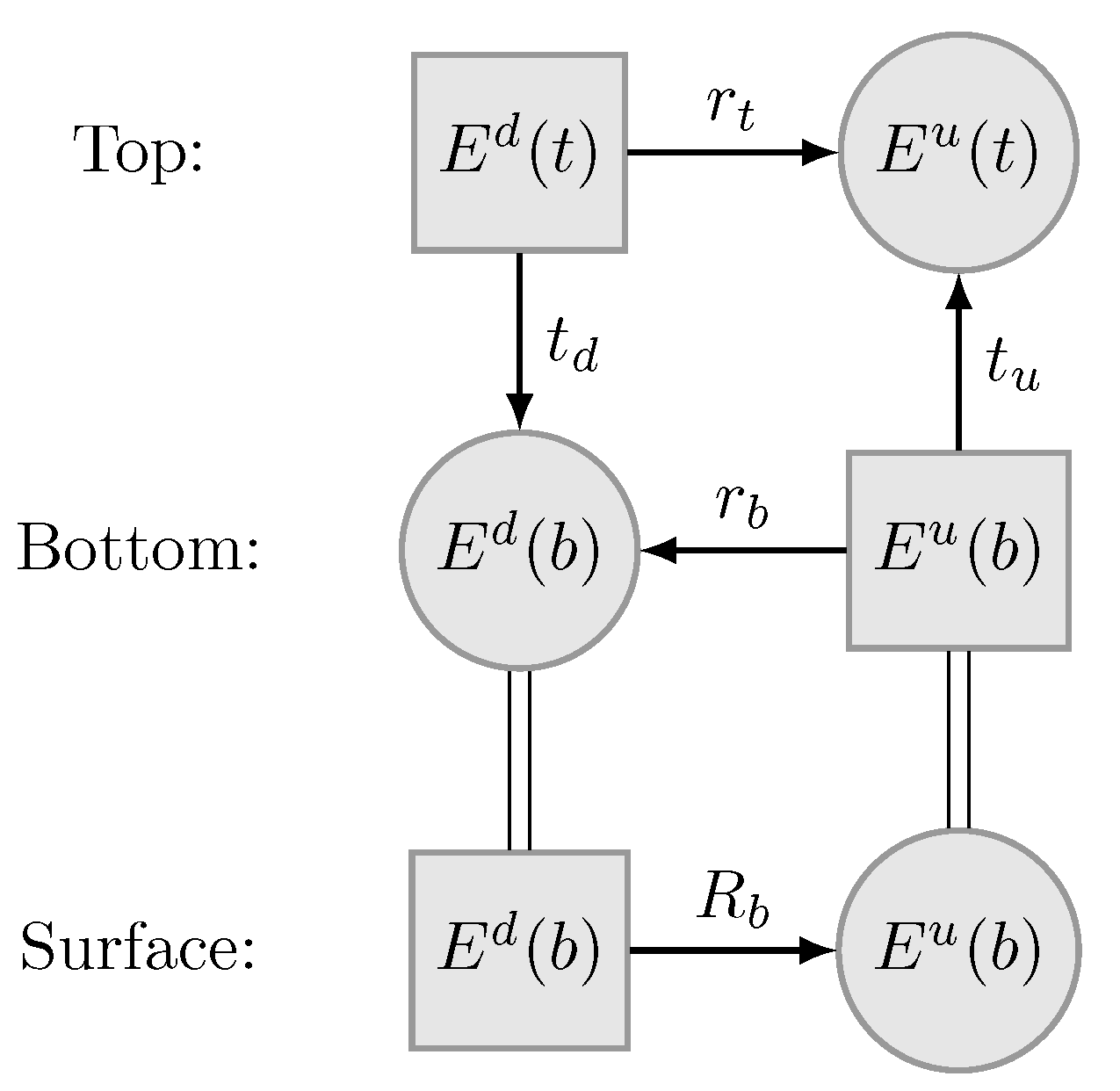
The radiative transfer of fluxes can be summarized in a similar way as in Figure 1, but now we consider that each layer may generate fluxes ($E_e^u$ and $E_e^d$) and the fluxes at the top of a surface may contain a reflected downward flux, as well as an upward emitted flux, called U. Figure 3 is a revised version of Figure 1 with contribution of thermal or fluorescence emission.

The following quantities are required to solve the system in Equation (14):

• scattering matrix of each elementary layer (i.e., $t_d$, $r_b$, $r_t$, and $t_u$),
• reflective properties of the system at all levels $R_t^{*}$,
• flux profiles inside the canopy $E_u$ and $E_d$ without the contribution of thermal and fluorescence emission,
• thermal emission ($E_{et}^d$ and $E_{et}^u$) of each elementary vegetation layer and soil $U_t\left(1\right)$,
• fluorescence emission ($E_{ef}^d$ and $E_{ef}^u$) of each elementary layer and soil $U_f\left(1\right)$,
• upward emitted thermal fluxes at all levels $U_t$,
• upward emitted fluorescence fluxes at all levels $U_f$,
• thermal flux profiles inside the canopy $E_t^d$ and $E_t^u$, and
• fluorescence flux profiles inside the canopy $E_f^d$ and $E_f^u$.

Because the computation of fluorescence emission normally requires knowing the excitation fluxes inside the canopy, the radiative transfer of fluorescence can only be solved when the radiative transfer of incident radiation is solved (i.e., $E_u$ and $E_d$ in the third item). Likewise, the temperatures are sometimes modeled as a function of the optical fluxes inside the fluxes (i.e., $E_u$ and $E_d$ in the third item), for example, with an energy balance approach as in the SCOPE model [19]. Nevertheless, the leaf temperatures are sometimes given as direct input. In this case, the radiative transfer of canopy emitted thermal radiation can be combined with radiative transfer of incident radiation.

The radiative transfer for either the incident, emitted fluorescence, and thermal radiation can all be represented by the system expressed as Equation (14). If only incident radiation is considered, then the emission of each layer and soil is set to zero. If the fluorescence and thermal emission from soil and foliage are zero (i.e., $E_e^d$, $E_e^u$ and $U\left(1\right)$ are zero), then it follows that the upward emitted fluxes at every level $U\left(j\right)$ all equal to zero. Therefore, the above presented theory is a unified radiative transfer theory for optical, thermal, and fluorescence in multi-layer canopies. In what follows, we first describe the general solution of such a system assuming thermal and fluorescence emission is known and then elaborate the computation of thermal and fluorescence emission afterwards.

3.2. Solution for Multi-Layer Canopies

3.2.1. Scattering Matrices of an Elementary Layer

For a thin layer, the scattering matrices can be directly computed from the extinction and scattering coefficients.

$$\left[\begin{array}{cc}{t}_d& r_b\\ r_t& t_u\end{array}\right]=\left[\begin{array}{cccc}1-k\delta L& & & \\ s^{\prime }\delta L& 1-a\delta L& \sigma \delta L& \\ s\delta L& \sigma \delta L& 1-a\delta L& \\ w\delta L& v\delta L& v^{\prime }\delta L& 1-K\delta L\end{array}\right],$$

(15)

where $\delta L$ is the LAI of a thin layer, which is canopy $L/N$. Note that all the scattering and extinction coefficients can vary vertically, as well as the reflectances and transmittances of the layer in the scattering matrix.

3.2.2. Solutions for a Surface-Layer System with Emission

The differences of fluxes at any two successive levels are affected by the thin layer between the two levels, and the thick layer under the lower level. This can be regarded as a surface-layer combination with surface reflectance $R_t^{*}\left(j\right)$ and upward emitted fluxes $U\left(j\right)$ and the layer scattering matrices ($t_d\left(j\right)$, $r_b\left(j\right)$, $r_t\left(j\right)$, $t_u\left(j\right)$), and the fluxes interactions between two successive levels can be expressed as:

$$\left[\begin{array}{c}{E}^d\left(j\right)\\ E^u(j+1)\end{array}\right]=\left[\begin{array}{cc}{t}_d\left(j\right)& r_b\left(j\right)\\ r_t\left(j\right)& t_u\left(j\right)\end{array}\right]\left[\begin{array}{c}{E}^d(j+1)\\ E^u\left(j\right)\end{array}\right]+\left[\begin{array}{c}{E}_e^d\left(j\right)\\ E_e^u\left(j\right)\end{array}\right],$$

(16a)

$$E^u\left(j\right)=R_t^{*}\left(j\right)E^d\left(j\right)+U\left(j\right).$$

(16b)

The relationship between the downward fluxes at successive levels, while taking into account both the multiple reflectance with and the emission from the thick layer, can be obtained by introducing Equation (16b) into Equation (16a):

$$\begin{array}{cc}\hfill E^d\left(j\right)& =T_d^{*}(j+1)E^d(j+1)+Y\left(j\right)\hfill \\ \hfill E^u(j+1)& =R_t^{*}(j+1)E^d(j+1)+U(j+1)\hfill \end{array},$$

(17)

where we find

$$\begin{array}{cc}\hfill Y\left(j\right)& ={[I-r_b\left(j\right)R_t^{*}\left(j\right)]}^{-1}[r_b\left(j\right)U\left(j\right)+E_e^d\left(j\right)]\hfill \\ \hfill U(j+1)& =t_u\left(j\right)[R_t^{*}\left(j\right)Y\left(j\right)+U\left(j\right)]+E_e^u\left(j\right)\hfill \\ \hfill T_d^{*}(j+1)& ={[I-r_b\left(j\right)R_t^{*}\left(j\right)]}^{-1}{t}_d\left(j\right)\hfill \\ \hfill R_t^{*}(j+1)& =r_t\left(j\right)+t_u\left(j\right)R_t^{*}\left(j\right)T_d^{*}(j+1)\hfill \end{array}.$$

(18)

The whole system can be solved with two recursive loops. The first loop computes the effective downward transmittance ($T_d^{*}$), surface reflectance ($R_t^{*}$), downward emission (Y), and upward emission (U) at all levels. The soil reflectance is known; thus, $R_t^{*}\left(1\right)=R_s$. The effective downward transmittance at the level of the soil surface is zero (i.e., $T_d^{*}\left(1\right)=0$). The upward fluorescence emission of soil is zero ($U_f\left(1\right)=0$). In the thermal domain, upward emission is dependent to soil temperature. A pseudo algorithm going from bottom to top is given as

After application of this algorithm from the bottom to the top of the canopy, the second loop is applied to derive the fluxes at all levels by using the relationship of fluxes between two successive levels. A pseudo algorithm going from top to bottom is given as the following.

The Algorithm 1 gives the optical properties of each layer and surface, while Algorithm 2 provides the flux profiles.

Algorithm 1 Calculate $T_d^{*}$, $R_t^{*}$, Y and U.

Require:$T_d^{*}\left(1\right)=0$, $R_t^{*}\left(1\right)=R_s$ and $U\left(1\right)$                     scattering matrices of every thin layer ($t_d$, $r_b$, $r_t$, $t_u$)                     thermal or fluorescence emission of each thin layer $E_e^u$ and $E_e^d$          loop               for $j\leftarrow 1$ to $N+1$              do Equation (18)            end loop

Algorithm 2 Calculate $E^d$, $E^u$.

Require:$T_d^{*}$, $R_t^{*}$, Y, U at every level                     downward fluxes at top of canopy $E^d(N+1)={\left[\begin{array}{cc}{E}_{sun}& E_{sky}\end{array}\right]}^T$          loop              for $j\leftarrow N+1$ to 1              do Equation (17)           end loop

3.3. Thermal and Fluorescence Emission of a Thin Layer

3.3.1. Thermal Emission

Thermal hemispheric emission of a leaf and the soil background ($U_t\left(1\right)$) can be computed according to the Planck’s law: $\epsilon \pi B(T,\lambda )$. B is Planck’s spectral radiance function for the indicated canopy temperature (T) and the associated wavelength $\lambda$, and $\epsilon$ is the emissivity of the object. Assuming that leaves emit thermal radiance isotropically and on both sides in equal amounts, the thermal emission by leaves are given as $E_{et}^b$ = $E_{et}^f$ =$\epsilon \pi B(T,\lambda )$, where the superscript b and f refer to backward and forward direction relatively to the incident light. Furthermore, this assumption indicates that thermal emission of a thin vegetation layer is isotropic and has the same amount on both sides of the layer.

For the emission in the viewing direction, we employ the coefficient K that projects a small leaf area on the plane perpendicular to the viewing direction. Therefore, the conversion of the diffuse emitted radiation $E_e^b$ and $E_e^f$ of individual leaves into those for the layer can be expressed as

$$E_{et}^u=\left[\begin{array}{c}{E}_{et}^{+}\\ E_o^{et}\end{array}\right]={\epsilon }_l\pi B(T_l,\lambda )\left[\begin{array}{c}1\\ K\end{array}\right]\delta L,$$

(19)

$$E_{et}^d=\left[\begin{array}{c}{E}_s^{et}\\ E_{et}^{-}\end{array}\right]={\epsilon }_l\pi B(T_l,\lambda )\left[\begin{array}{c}0\\ 1\end{array}\right]\delta L,$$

(20)

where ${\epsilon }_l$ and $T_l$ are the leaf emissivity and temperature, respectively. $E_{et}^{+}$ and $E_{et}^{-}$ are upward and downward diffuse irradiance, and $E_o^{et}$ is equivalent thermal irradiance in the viewing direction. $E_s^{et}$ is direct solar thermal irradiance emitted from the leaves, which is null for leaves and set to zero in the calculation. It is given in the above equations for the sake of the competence of the four-stream theory.

The upward emitted thermal fluxes by soil surface can be computed in the same way as

$$U_t\left(1\right)=\left[\begin{array}{c}{E}_{et}^{+}\\ E_o^{et}\end{array}\right]={\epsilon }_s\pi B(T_s,\lambda )\left[\begin{array}{c}1\\ 1\end{array}\right],$$

(21)

where ${\epsilon }_s$ and $T_s$ are the soil emissivity and temperature, respectively.

3.3.2. Fluorescence Emission

Fluorescence emission of a thin layer is excited by the direct solar flux ($E_s$), upward ($E^{+}$), and downward ($E^{-}$) diffuse light at each spectral band (${\lambda }_e$) from 400 to 700 nm. One can simulate the upward and downward fluorescence emission for a given irradiance of a thin layer and a fluorescence emission efficiency. The source terms due to fluorescence emission by leaves are given as

$$\begin{array}{cc}\hfill E_{ef}^{-}=& {\int }_{400}^{700}[s_f^{\prime }{E}_s+{\sigma }_f^{\prime }{E}^{-}+{\sigma }_f{E}^{+}]d{\lambda }_e\delta L,\hfill \end{array}$$

(22a)

$$\begin{array}{cc}\hfill E_{ef}^{+}=& {\int }_{400}^{700}[s_f{E}_s+{\sigma }_f{E}^{-}+{\sigma }_f^{\prime }{E}^{+}]d{\lambda }_e\delta L,\hfill \end{array}$$

(22b)

$$\begin{array}{cc}\hfill E_o^{ef}=& {\int }_{400}^{700}[w_f{E}_s+v_f{E}^{-}+v_f^{\prime }{E}^{+}]d{\lambda }_e\delta L,\hfill \end{array}$$

(22c)

where the excitation-emission coefficients (with subscript f) are determined by sun-observer geometry, canopy structure, leaf optical properties, and fluorescence emission efficiency of photosystems, as given in Reference [9].

The fluxes ($E_s$, $E^{+}$ and $E^{-}$) at each elementary layer are computed as described in Section 3.2. The excitation-emission coefficients with subscript f can be found in

Table 3. Emission coefficients for the possible combinations of incident ($E_1$) and emitted fluorescence ($E_2$, with notation “ef”) flux of single leaves.

	${\mathit{E}}_1$	${\mathit{E}}_{\mathit{s}}$		${\mathit{E}}^{-}$	${\mathit{E}}^{+}$
${\mathit{E}}_2$		${\mathit{f}}_{\mathit{s}}>\mathbf{0}$	${\mathit{f}}_{\mathit{s}}<\mathbf{0}$
		$E_{ef}^{-}$		$f_s(M_f{f}_1+M_b{f}_2)$	$-f_s(M_b{f}_1+M_f{f}_2)$	$f_1(M_f{f}_1+M_b{f}_2)+f_2(M_b{f}_1+M_f{f}_2)$	$f_1(M_b{f}_1+M_f{f}_2)+f_2(M_f{f}_1+M_b{f}_2)$
$E_{ef}^{+}$		$f_s(M_b{f}_1+M_f{f}_2)$	$-f_s(M_f{f}_1+M_b{f}_2)$	$f_1(M_b{f}_1+M_f{f}_2)+f_2(M_f{f}_1+M_b{f}_2)$	$f_1(M_f{f}_1+M_b{f}_2)+f_2(M_b{f}_1+M_f{f}_2)$
$E_o^{ef}$	$f_o>0$	$f_s{M}_b{f}_o$	$-f_s{M}_f{f}_o$	$(M_b{f}_1+M_f{f}_2)f_o$	$(M_f{f}_1+M_b{f}_2)f_o$
	$f_o<0$	$-f_s{M}_f{f}_o$	$f_s{M}_b{f}_o$	$-(M_f{f}_1+M_b{f}_2)f_o$	$-(M_b{f}_1+M_f{f}_2)f_o$

$M_b$ and $M_f$ are the excitation-emission matrices of leaves in the back and forward direction (relative to the incident light), respectively.

, which, by analogy, are related to the corresponding scattering coefficients in Table 2. The excitation-emission matrices $M_b$ and $M_f$ are analogous to leaf reflectance and transmittance, respectively. The difference is that reflectance and transmittance describe the relationship between incident radiation and outgoing scattered radiation of a leaf, while the matrices describe the relationship between incident radiation and outgoing emitted radiation of a leaf. In a scattered event, the wavelength of an incident radiation and outgoing radiation remains the same, but, in a emission event, the emitted radiation is of different wavelength than the incident.

3.4. Illustrative Simulations

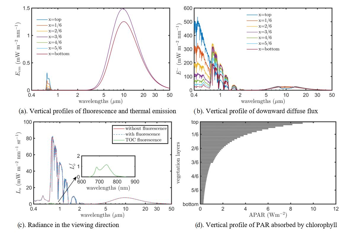
To demonstrate the capability of the present theory, we carry out an illustrative simulation. The setting of the scenarios is briefly described as follows. A vegetation canopy with two distinctive layers, of which the upper layer consists of leaves with high chlorophyll content ($C_{ab}=80$$\mathsf{\mu }$g cm${}^{-2}$) and the lower with $C_{ab}=20$$\mathsf{\mu }$g cm${}^{-2}$. The emissivity of the leaves in the canopy is set to 0.95. Moreover, the temperature of the leaves in the upper layer is set to 25 ${}^{\circ }$C and the lower 15 ${}^{\circ }$C. Besides leaf chlorophyll content and temperature, other properties of the two layers are identical. Specifically, both layers have LAI of 1.5 (i.e., total canopy is 3) and have spherical leaf angle distribution. The sun-observer geometry is defined as ${\theta }_s={30}^{\circ }$ and ${\theta }_v=0^{\circ }$.

The unified four-stream theory resolves the radiative transfer in vegetation canopies, and the profiles for fluorescence and thermal emission, upward, and downward diffuse fluxes, and vegetation absorption, as well as outgoing directional radiation, are simulated as shown in Figure 4. Different leaf chlorophyll content and leaf temperature of the two layers result in different leaf optical properties (Figure 4a) and thermal emission (Figure 4b), respectively. Furthermore, the fluorescence emission clearly shows vertical variation (the spectral region from 640 to 850 nm in Figure 4b). This is mainly affected by vertical variation of the radiation inside the vegetation canopy as shown in Figure 4c,d. The radiation in the photosynthetically active radiation (PAR) region for the downward diffuse flux decreases from top to bottom due to the strong absorption in this region (Figure 4c). The absorption of PAR decreases gradually from the top to the bottom of the canopy (Figure 4e). An abrupt change of absorbed PAR (APAR) occurs in the middle of the canopy (i.e., $x=1/2$) because of the change of high chlorophyll content of the upper layer to low chlorophyll content of the lower layer. Lastly, the radiance observed in the viewing direction is simulated, as well (Figure 4f), which can be used to compute canopy reflectance. Note the simulation results cover the spectral region from 0.4 $\mathsf{\mu }$m to 50 $\mathsf{\mu }$m and are in 1 nm spectral resolution, but other spectral resolutions are also possible for this unified theory.

4. Discussion

4.1. Hot Spot Effects for Remote Sensing Applications

This note presents a theory for the simulation of all the four streams, including fluxes in the viewing direction, which supports remote sensing applications. The fluxes inside the canopy can be used to predict net radiation and photosynthesis. Hence, this theory can be applied as a component in vegetation energy balance, photosynthesis, or physiological models.

However, in this report, the hot spot effect on fluxes in the viewing direction ($E_o$) is not considered. The hot spot effect is caused by the preferential reflectance (or emission) of a surface in the opposite direction to the incident radiation. This leads to an enhanced brightness in that direction relative to other directions. In a vegetated surface consisting of optically isotropic leaves and soil, the hotpot is caused by the coincidence of exposure to incident radiation and the direct transmittance of scattered radiation in opposite direction. In other words, if the incident radiation reaches a leaf by direct transmittance, then the scattered radiation can directly escape the canopy following the reversed path. The probability of direct transmittance may also be enhanced in directions close to this path, i.e., angles close to the incident angle. The range of angles in which the direct transmittance is enhanced determines the size of the hotspot (in angular units), which increases with the size of the objects (leaves) relative to the vegetation height. The radiative transfer theory presented in this report uses a turbid medium representation of the vegetation. In this representation, leaves are infinitely small, and the preferential reflectance only occurs the exact incident direction, such that the hotspot is infinitely small.

Accounting for the variation of $E_o$ in the horizontal plane caused by the hot spot effects in vegetation with leaves of a determined size requires further geometrical modeling and accounting for co-variances of projections in incident and viewing direction. One can compute $E_o$ separately by combining the four-stream theory with Kuusk’s approach for the hot spot effect [16,23].

4.2. Vertical Distribution of Leaf Area

We have considered the vertical variation of leaf optical properties and leaf orientations, which are expressed by the scattering and extinction coefficients of layers. In contrast, the distribution of leaf density in the vertical direction was not considered. Figure 2 depicts a uniform vertical distribution of leaves in the canopy, but a non-uniform arrangement of leaves in the vertical direction is very common in reality.

The radiative transfer theory presented here uses units of leaf area index ($Ldx$), rather than height above the soil surface, to define the depth of the canopy. The solution of the differential equations (Equation (1)) is therefore indifferent to the ways that the leaf area is distributed in the vertical direction. Thus, the use of a turbid medium representation of the canopy leads to the counterintuitive conclusion that the radiative transfer is indifferent to the vertical arrangement of leaf density.

However, one can imagine cases in which this is not the case, and the vertical distribution of leaf area matters for the radiative transfer. First, if optical properties are assigned to the air space between the leaves, then the optical properties of a layer are no longer determined by the properties of leaves alone. In that case, the vertical distribution of leaf density will affect the properties of the layers because the contribution of air to the layer properties will scale inversely with the leaf area density. Since the theory allows for layer properties to vary vertically, this can be accounted for easily by assigning appropriate layer properties. Second, if the objective is to model the hotspot or the position of sunlit and shaded locations in the canopy, then the turbid medium representation does not suffice. In that case, the theory can be blended with an approach to model specific effects of geometrical shapes. Apart from radiative transfer, the vertical distribution of leaf area also affects the physiology of vegetation via its effect on turbulent heat and matter exchanges and hydraulic pressure in the vegetation.

4.3. Applications to Other Systems

The theory is an extension of the classical four-stream theory to accommodate vertical heterogeneity of leaf properties and orientations in vegetation canopies (i.e., soil-vegetation systems). The modeling concept, however, has potential in radiative transfer modeling in media other than vegetation, such as water and atmosphere, which have a clear multi-layer structure [16,24]. The main differences are in the derivation of scattering, extinction, and excitation-emission coefficients of the sub-layers. Once these coefficients are derived for each layer, the solution of the system can be solved by using the solutions presented in this report (Equations (17) and (18)).

Additionally, the unified four-stream theory can be used to solve the radiative transfer problems in soil-water, soil-vegetation, soil-water-atmosphere, or soil-vegetation-atmosphere ensembles [25]. These ensembles can be considered as a multi-layer system. For example, compared with the soil-vegetation system presented in this report, the application of the unified theory to a soil-water system in coastal areas can be achieved by replacing the vegetation layer with a water layer. The radiative transfer problems in a soil-vegetation-atmosphere can be solved by adding an atmosphere layer on top of a soil-vegetation system.

References

1. Jacquemoud, S.; Baret, F. PROSPECT: A model of leaf optical properties spectra. Remote Sens. Environ. 1990, 34, 75–91. [Google Scholar] [CrossRef]
2. Li, X.; Strahler, A.H. Geometric-optical bidirectional reflectance modeling of a conifer forest canopy. IEEE Trans. Geosci. Remote Sens. 1986, 906–919. [Google Scholar] [CrossRef]
3. Ni, W.; Li, X.; Woodcock, C.E.; Caetano, M.R.; Strahler, A.H. An analytical hybrid GORT model for bidirectional reflectance over discontinuous plant canopies. IEEE Trans. Geosci. Remote Sens. 1999, 37, 987–999. [Google Scholar]
4. Allen, W.A.; Gayle, T.V.; Richardson, A.J. Plant-canopy irradiance specified by the Duntley equations. JOSA 1970, 60, 372–376. [Google Scholar] [CrossRef]
5. Suits, G.H. The calculation of the directional reflectance of a vegetative canopy. Remote Sens. Environ. 1971, 2, 117–125. [Google Scholar] [CrossRef] [Green Version]
6. Verhoef, W. Light scattering by leaf layers with application to canopy reflectance modeling: The SAIL model. Remote Sens. Environ. 1984, 16, 125–141. [Google Scholar] [CrossRef] [Green Version]
7. Kuusk, A. A two-layer canopy reflectance model. J. Quant. Spectrosc. Radiat. Transf. 2001, 71, 1–9. [Google Scholar] [CrossRef]
8. Wang, Q.; Li, P. Canopy vertical heterogeneity plays a critical role in reflectance simulation. Agric. For. Meteorol. 2013, 169, 111–121. [Google Scholar] [CrossRef]
9. Yang, P.; Verhoef, W.; Van der Tol, C. The mSCOPE model: A simple adaptation to the SCOPE model to describe reflectance, fluorescence and photosynthesis of vertically heterogeneous canopies. Remote Sens. Environ. 2017, 201, 1–11. [Google Scholar] [CrossRef]
10. Gastellu-Etchegorry, J.P.; Demarez, V.; Pinel, V.; Zagolski, F. Modeling radiative transfer in heterogeneous 3-D vegetation canopies. Remote Sens. Environ. 1996, 58, 131–156. [Google Scholar] [CrossRef] [Green Version]
11. North, P.R. Three-dimensional forest light interaction model using a Monte Carlo method. IEEE Trans. Geosci. Remote Sens. 1996, 34, 946–956. [Google Scholar] [CrossRef]
12. Disney, M.; Lewis, P.; North, P. Monte Carlo ray tracing in optical canopy reflectance modelling. Remote Sens. Rev. 2000, 18, 163–196. [Google Scholar] [CrossRef]
13. Knyazikhin, Y.V.; Marshak, A.L.; Myneni, R.B. Interaction of photons in a canopy of finite-dimensional leaves. Remote Sens. Environ. 1992, 39, 61–74. [Google Scholar] [CrossRef]
14. Gastellu-Etchegorry, J.P.; Yin, T.; Lauret, N.; Cajgfinger, T.; Gregoire, T.; Grau, E.; Feret, J.B.; Lopes, M.; Guilleux, J.; Dedieu, G.; et al. Discrete anisotropic radiative transfer (DART 5) for modeling airborne and satellite spectroradiometer and LIDAR acquisitions of natural and urban landscapes. Remote Sens. 2015, 7, 1667–1701. [Google Scholar] [CrossRef] [Green Version]
15. Verhoef, W. Earth observation modeling based on layer scattering matrices. Remote Sens. Environ. 1985, 17, 165–178. [Google Scholar] [CrossRef] [Green Version]
16. Verhoef, W. Theory of Radiative Transfer Models Applied in Optical Remote Sensing of Vegetation Canopies; Wageningen University: Wageningen, The Netherlands, 1998. [Google Scholar]
17. Verhoef, W.; Jia, L.; Xiao, Q.; Su, Z. Unified optical-thermal four-stream radiative transfer theory for homogeneous vegetation canopies. IEEE Trans. Geosci. Remote Sens. 2007, 45, 1808–1822. [Google Scholar] [CrossRef]
18. Zarco-Tejada, P.J.; Miller, J.R.; Pedrós, R.; Verhoef, W.; Berger, M. FluorMODgui V3. 0: A graphic user interface for the spectral simulation of leaf and canopy chlorophyll fluorescence. Comput. Geosci. 2006, 32, 577–591. [Google Scholar] [CrossRef] [Green Version]
19. Van der Tol, C.; Verhoef, W.; Timmermans, J.; Verhoef, A.; Su, Z. An integrated model of soil-canopy spectral radiances, photosynthesis, fluorescence, temperature and energy balance. BIogeosciences 2009, 6, 3109–3129. [Google Scholar] [CrossRef] [Green Version]
20. Van der Tol, C.; Vilfan, N.; Dauwe, D.; Cendrero-Mateo, M.P.; Yang, P. The scattering and re-absorption of red and near-infrared chlorophyll fluorescence in the models Fluspect and SCOPE. Remote Sens. Environ. 2019, 232, 111292. [Google Scholar] [CrossRef]
21. Farquhar, G.D.; von Caemmerer, S.V.; Berry, J.A. A biochemical model of photosynthetic CO2 assimilation in leaves of C3 species. Planta 1980, 149, 78–90. [Google Scholar] [CrossRef] [Green Version]
22. Verhoef, W.; Bach, H. Coupled soil–leaf-canopy and atmosphere radiative transfer modeling to simulate hyperspectral multi-angular surface reflectance and TOA radiance data. Remote Sens. Environ. 2007, 109, 166–182. [Google Scholar] [CrossRef]
23. Kuusk, A. The hot spot effect in plant canopy reflectance. In Photon-Vegetation Interactions; Springer: Berlin/Heidelberg, Germany, 1991; pp. 139–159. [Google Scholar]
24. Salama, M.S.; Verhoef, W. Two-stream remote sensing model for water quality mapping: 2SeaColor. Remote Sens. Environ. 2015, 157, 111–122. [Google Scholar] [CrossRef] [Green Version]
25. Yang, P.; van der Tol, C.; Yin, T.; Verhoef, W. The SPART model: A soil-plant-atmosphere radiative transfer model for satellite measurements in the solar spectrum. Remote Sens. Environ. 2020, 247, 111870. [Google Scholar] [CrossRef]
Figure 1. Flux interaction diagram for the combination of a vegetation layer on top of a reflecting surface (e.g., soil). A rectangle stands for incident radiation and a circle for reflected or transmitted radiation. The rectangles and circles are connected by arrows that indicate the direction of flow, and a symbol next to the arrow indicates the corresponding reflectance or transmittance. The notations t and b in the brackets indicate the top of and bottom of a vegetation layer, respectively. r and t are the reflectance and transmittance matrices where the subscripts attached to the matrices denote downward (d), upward (u), top (t), and bottom (b) (i.e., r t and r b are the reflectance at top and bottom of the vegetation layer, respectively. t d and t u are the downward and upward transmittance, respectively).
Remotesensing 12 03914 g001
Figure 2. Homogeneous (a) and multi-layer canopies with vertical heterogeneity of leaf optical properties and orientations (b). Numbering the layers (solid arrows) and flux levels (dashed arrows) for applying the four-stream theory to multi-layer canopies (c).
Remotesensing 12 03914 g002
Figure 3. Flux interaction diagram for the emitted radiation in a system of a vegetation layer on top of a reflecting surface (e.g., soil). U indicates the upward emitted fluxes at a surface. E e u and E e d are the upward and downward emission of the vegetation layer.
Remotesensing 12 03914 g003
Figure 4. Illustration of the capability of the unified four-stream radiative transfer theory in the spectral region from 0.4 to 50 μ m. (a) Leaf reflectance and transmittance of the leaves in the two layers. (b) Vertical profiles of fluorescence and thermal emission. (c) Vertical profile of downward diffuse flux. (d) Vertical profile of upward diffuse flux. (e) Vertical profile of photosynthetically active radiation (PAR) absorbed by chlorophyll. (f) Radiance in the viewing direction.
Remotesensing 12 03914 g004