Abstract
The Markov Random Field (MRF) energy function, constructed by existing OpenMVS-based 3D texture reconstruction algorithms, considers only the image label of the adjacent triangle face for the smoothness term and ignores the planar-structure information of the model. As a result, the generated texture charts results have too many fragments, leading to a serious local miscut and color discontinuity between texture charts. This paper fully utilizes the planar structure information of the mesh model and the visual information of the 3D triangle face on the image and proposes an improved, faster, and high-quality texture chart generation method based on the texture chart generation algorithm of the OpenMVS. This methodology of the proposed approach is as follows: (1) The visual quality on different visual images of each triangle face is scored using the visual information of the triangle face on each image in the mesh model. (2) A fully automatic Variational Shape Approximation (VSA) plane segmentation algorithm is used to segment the blocked 3D mesh models. The proposed fully automatic VSA-based plane segmentation algorithm is suitable for multi-threaded parallel processing, which solves the VSA framework needed to manually set the number of planes and the low computational efficiency in a large scene model. (3) The visual quality of the triangle face on different visual images is used as the data term, and the image label of adjective triangle and result of plane segmentation are utilized as the smoothness term to construct the MRF energy function. (4) An image label is assigned to each triangle by the minimizing energy function. A texture chart is generated by clustering the topologically-adjacent triangle faces with the same image label, and the jagged boundaries of the texture chart are smoothed. Three sets of data of different types were used for quantitative and qualitative evaluation. Compared with the original OpenMVS texture chart generation method, the experiments show that the proposed approach significantly reduces the number of texture charts, significantly improves miscuts and color differences between texture charts, and highly boosts the efficiency of VSA plane segmentation algorithm and OpenMVS texture reconstruction.
1. Introduction
Over the last two decades, 3D modeling from low-altitude oblique images has been used in a wide range of applications, including urban planning, tourism, and computer vision. 3D image-modeling technology primarily involves generating two kinds of reconstruction, the 3D model object [1,2,3,4,5] and its texture. To improve the visual realism of the model, the former increases the complexity of the model object, while the latter improves the precision of the texture mapping. Without increasing the model’s geometric complexity, accurate and reliable texture reconstruction is essential to achieve visual realism. Many sophisticated methods have been proposed for texture reconstruction. However, local miscuts and color discontinuity caused by vast texture chart fragments continue to be major challenges in the realistic texturing of models.
The texture chart is the basic unit of texture reconstruction, which is a connected region of the triangle mesh [6,7,8], and its main task is to map the model surface into a 2D image domain. Texture chart can establish the index relationship between the triangle face in the mesh model and texture image corresponding to the texture chart. The texture information of all faces in a texture chart comes from the same image. Color miscuts and discontinuity between the texture chart will cause a visual seam-line. The seam-line of adjacent texture charts has a different slope and texture scale in images, resulting in the inaccurate initial value of the color adjustment algorithm and influencing the model’s rendering effect at the texture chart boundary. The problem becomes more evident as the number of texture charts increases.
Texture reconstruction is the process of calculating and executing the image-to-geometry registration, which generally includes multiple techniques, such as mesh segmentation, texture transferring, and correction and optimization. Mesh segmentation generates texture charts, which is crucial in 3D texture reconstruction and will directly affect subsequent steps. Most texture chart generation approaches use the MRF energy function to assign an image label for each triangle face. Then, the topologically adjacent triangle faces with the same label are aggregated into texture charts [7,9,10,11,12,13,14]. The energy function contains the data term and the smoothness term. The main purpose of the data term is to select a high-resolution image (the image clarity) and reduce chart-to-chart miscuts to a certain extent. Intuitively, the purpose of the smoothness term is to reduce the number of texture charts and the overall color discontinuity, which can effectively improve the efficiency of subsequent texture mapping steps, and even have a better promotion effect on the future application of real-time dynamic local texture mapping visualization (3D texture model visualization). In addition, it can minimize the sampling error of the texture chart boundary seam-line to a certain extent.
The plane is basic geometric structure information in the model. Triangle faces in the same plane are easier to maintain a similar visual quality on the same image. In this paper, the plane is used as a constraint condition to limit the results of texture chart generation. Many scholars [15,16,17,18,19] introduced the Variational Shape Approximation (VSA) framework, which segments the input mesh surface into planar charts. The quality of the segmentation is measured by the sum of the derivation of each chart from its corresponding planar proxy. The VSA framework needs to manually set the number of charts, which is easy to do for small data models (such as Computer-Aided Design (CAD) parts) but not for large data models (such as an entire city). For each model, the number of texture charts required is different. The VSA results lack image information and cannot be used directly in the texture reconstruction process.
Open Multi-View Stereovision (OpenMVS) [20] is an open-source 3D reconstruction program that uses MRF energy function in texture reconstruction. This paper fully utilizes the planar structure information of the mesh model and the visual information of the 3D triangle face on the image and provides an improved, faster, and high-quality texture chart generation method based on the OpenMVS texture chart generation algorithm. Improvements include: adding improved VSA plane segmentation, modifying the smoothness term of the MRF energy function, and optimizing the boundary seam-line problem of texture charts. Using the method proposed in this paper, the number of generated texture chart fragments greatly reduces, which will help solve the problem of miscutting and large color discontinuity between texture charts, and will help to improve the efficiency of subsequent texture mapping steps and the visual expression of 3D texture models. Compared with the original OpenMVS texture chart generation method, this paper’s method achieves the following three goals: (1) improving the operating efficiency of the OpenMVS texture chart generation method to a certain extent; (2) reducing the number of texture charts (it helps ameliorate the problem by miscuts and large color discontinuity between texture charts); (3) to a certain extent, minimizing the sampling error of the boundary seam-line of texture charts.
The remainder of this paper is organized as follows. Section 2 introduces the related work of texture chart generation. Section 3 describes the texture reconstruction method of OpenMVS. In Section 4, we explain our proposed improved texture reconstruction method based on the block VSA fully automatic plane segmentation algorithm. Experiments and discussion are described and analyzed in Section 5. Conclusions are drawn in Section 6.
2. Related Works
2.1. 3D Texture Reconstruction
Blending-based method: It is the simplest method of texture mapping. Bi et al. [7], Callieri et al. [21], and Hoegner et al. [22] projected the captured images onto the surface of the geometric model according to the intrinsic and extrinsic orientation parameters of the camera and then merged all the images to obtain the final texture image. This method is suitable for processing close-range and small-range models, such as indoor scenes and small objects. It requires high calculation accuracy. The blurring and ghosting will easily emerge if the recovered camera poses or the 3D geometry model is slightly inaccurate. Besides, the process of model subdivision and model size in different perspectives also affect the texture reconstruction effect.
Parameterization-based method is the process of segmenting the model surface under certain rules (equal-area mapping, conformal mapping, minimum deformation [8,23,24,25]) and mapping the 3D mesh model to the 2D texture image domain. It computes the texture coordinate for each triangle face. This method generates small amounts of texture charts, but the 2D texture image domain is deformed compared to the original image, which will inevitably cause the loss of texture information and is not conducive to improving the texture reconstruction effect. Moreover, the triangle face in the same texture chart is invisible or has poor visual quality on the same image. Other standards (such as normal vector [26], area of the triangle face projected on the image [27]) are still required to assign an image label for each triangle face.
Projection-based method is projective texture mapping, which associates each triangle face with one image label, and then selects the topologically-adjacent triangle face with the same image label to form a texture chart. Lempitsky et al. [28] first proposed to use the MRF energy function to select an optimal image for each triangle face. On this basis, Fu et al. [29] and Li et al. [30] improved the data term of the energy function, and the image clarity was used as the value of the data term. Yang et al. [31] sampled the image sequence by using the spatio-temporal adaptive method. This method is a projection transformation from the model surface to the input image, which constitutes the optimal and most natural mapping. Compared with the blending-based method and parameterization-based method, the ghosting and the loss of texture information caused by the deformation are avoided.
The MRF energy function can avoid the discretization of label selection to a certain extent. However, the current smoothness terms of the MRF energy function are not fully considered, which will still result in a large number of texture chart fragments. Furthermore, there are generally serious local miscuts and color differences between texture charts, which reduces the execution efficiency of the texture mapping process.
2.2. Plane Structure Feature Segmentation
Plane structure feature segmentation is to segment the mesh model into planes based on the geometric attribute of the model.
The region growing approach is one of the most widely used segmentation methods. This method [32,33,34,35,36] selects a set of seed faces under certain rules and then grows around each seed face until all faces are assigned to a single region. When expanding a region, the local surface features are the main criteria. This method can separate the model well along high curvatures, but for surfaces with smooth curvatures (e.g., flat ellipse), this approach causes excessive planes.
The hierarchical approach comprises two main techniques: One way is the bottom-up region merging method [37,38,39,40]. This method assigns each face as a chart. In each step, a pair of adjacent charts with the least merging error is merged to form a new chart. The steps are repeated until the stop merging criteria are met. The merging criteria usually make use of the angle of the region normal vector, as proposed by Garland et al. [41]. This approach may encounter problems when blending charts with two smooth surfaces, merged in the early stages. Another technique is the gradual subdivision from top to bottom. Splitting algorithms [42,43] are based on the minima rule and part salience theory. The feature curves on mesh surfaces are first detected and used as segmentation criteria. Bi et al. [7], Kaiser et al. [44], and Yi et al. [45] defined various metrics for different application scenarios and subdivided them based on Cheng’s results. Since this approach tends to subdivide meshes in the concave region, many meaningful parts may be over-segmented.
Both the region growing approach and the hierarchical approach essentially belong to the same type of algorithm, where once the segmentation is done for a triangle face, it will not be changed in the subsequent process. However, mesh segmentation can also be treated as an energy minimization problem, where an energy function is defined and optimized for the segmentation. The planarity of the surface chart is usually used as error metrics to define the energy functions [16,17,46,47] in texture reconstruction. Because of its optimization nature, this method is often referred to as the variational method. Generally, the variational method provides better segmentation quality than the other approach.
The variational approach. Cohen-Steiner et al. [16] firstly proposed a VSA framework with minimal approximation errors. This framework uses the angle or distance between the face and the plane as the error term, and consistent energy minimization is applied to drive down the approximation error. A distortion minimization flooding algorithm is designed to keep the connectivity for each region. For different application scenarios, many types of surface element features were also introduced to extend this segmentation method. Kaiser et al. [44], Quan et al. [48], and Simari et al. [49] used the ellipsoid surface as an approximate plane to segment the ellipsoid area in the model by minimizing combined energy functions. Sun et al. [47], Wu et al. [50], and Thul et al. [51] also adopted a similar method and introduced spheres, cylinders, and rolling spheres as several basic approximate shapes. These methods have achieved good results in fitting known planes, but there may be under-segmenting or over-segmenting for different types of surface elements. Moreover, because this approach needs to manually set the number of charts, an automated setting method needs to be incorporated when used in urban texture reconstruction to provide automatic segmentation.
3. OpenMVS Texture Reconstruction Method
The texture reconstruction method of OpenMVS is based on the MRF energy function [52]. The energy function contains two parts: data term and smoothness term . The data term prefers high-quality views (visual quality) for texturing a face. The scoring formula for visual quality is expressed in Equation (1):
where is the area occupied by the faces projected on the image; is the number of all grid points obtained by rasterizing the projection result of ; is the gradient value of each grid point of on the image labeled ; and is the score of the on the image labeled .
The smoothness term minimizes seam (edges between faces textured with different images) visibility. The value is determined by the image label selected by the adjacent face. If the same image is selected for adjacent triangles, value is 0, and if different images are selected for the adjacent faces, value is infinite value.
At last, the energy function is minimized by graph-cut to assign the image label for each face, and the topologically adjacent triangles with the same label are aggregated into a texture chart. In addition, OpenMVS used the MVE‘s [12] method to adjust the texture chart color and packed the image information corresponding to the texture chart to output the texture image.
4. Improved Texture Reconstruction Method Based on the Fully automatic Plane Segmentation
This paper proposes an improved OpenMVS texture chart generation algorithm. Improvements include: (1) adding a fully automatic VSA-based plane segmentation algorithm for blocked 3D mesh models, which uses the degree of planar approximate error change as the standard for fully-automatic plane segmentation and realizes the multi-threaded parallel processing of the VSA algorithm by partition and merging the meshes after plane segmentation; (2) modifying the smoothness term of the MRF energy function, which combines the planar-structure information of the mesh model and the visual information to generate texture chart; and, (3) providing strategies for optimizing the jagged boundary problem of the texture chart. The flowchart of our algorithm is shown in Figure 1.
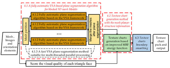
Figure 1.
Flowchart of improved texture reconstruction method based on the fully automatic plane segmentation.
4.1. A Fully Automatic VSA-Based Plane Segmentation Algorithm for Blocked 3D Mesh Models
In this step, the VSA framework is adopted as the basic method for extracting the model’s planar structural feature. The efficiency and effects of the VSA framework are improved by analyzing the deficiencies of the framework in processing models.
4.1.1. The VSA Framework
The overall segmentation strategy of the VSA framework includes two steps: First, the entire model is taken as the initial plane, and the framework is used in calculating the approximate error of the initial plane. The approximate error of the plane is the accumulation of the approximate error from each face to the planar proxy. The seed face of the plane is the face with the smallest approximation error. Yan et al. [17] provided two approximation error calculation methods (, ), which are based on the distance from the face to the planar proxy and the angle between the normal vectors of the face and planar proxy. Given a planar surface represented by , refers to the plane passing through of normal . The normal of the plane is the normal of the corresponding seed face. The error function for a plane is expressed as:
where , , are the orthogonal distances from three vertices of to the plane. and are the normal vector and area of each face, and is the normal vector of a planar proxy.
Next, the face with the largest error of all the planes is selected as a new seed face, and the Distortion-minimizing Flooding method is used to grow around the seed faces of the mesh. This step is repeated until the number of planes reaches a pre-specified tolerance (user manual setting). Since the seed face represents the proxy plane, all the approximate errors need to be recalculated after a new proxy plane is added. The seed face would be updated using the smallest error face for each plane.
4.1.2. Fully Automatic Plane Segmentation Algorithm Based on the VSA Framework
The number of planes in the VSA framework needs to be set manually. Achieving great results would be difficult when the set number of planes is insufficient. The number of planes required for different models varies considerably, and the fixed number of planes lacks versatility. This study proposes a fully automatic plane segmentation algorithm based on the VSA framework, which uses the change in the plane error as the stopping segmentation criteria after adding a new plane. We take as the error function for the plane. Since the images are taken by oblique photography, close faces are more likely to maintain a similar degree of deformation on the same image. The texture charts should be approximate to a connected plane. Mathematically, the computational cost of the approximate procedure using the normal vector is smaller than the distance. The formula is defined as:
where and are the error drop ratio before and after adding a new plane. The value of is the ratio of to , where is the error sum of all current planes and is the error of the initial plane (same as ). is the difference between the and . The smaller indicates that the segmentation result is more approximate a plane. With the number of planes increasing, and gradually decrease. declines until it is less than the threshold ( in all our experiments), which then stops the addition of new planes. At this point, all the planes have been extracted, and the mesh is segmented by the planes. The segmentation result is shown in Figure 2. Different planes are marked with different colors in each picture. Figure 2a shows the raw RGB model. Figure 2b displays the segmentation results when using a fixed value of 500. Some objects are not segmented, such as roof and plants on the ground. Figure 2c presents the results when the planes are dynamically increased. Unlike in Figure 2b, the main objects are extracted appropriately.

Figure 2.
Segmentation results were generated by two methods: (a) raw RGB model; (b) fixed the number of planes; (c) dynamically increasing the plane.
4.1.3. A Fast VSA Plane Segmentation Method Suitable for Multi-Threaded Parallel Processing
In the segmentation process, each time a new plane is added, the errors of all planes need to be recalculated. Parallel processing is not suitable for this algorithm, which means that the computer is not able to perform at its maximum performance. To deal with parallelism, the model is split into multiple blocks on the XOY plane, and then the algorithm uses multi-threading to fully automatically segment the planes of blocks at the same time. The range of each block is approximately equal, and the number of blocks is set by the user or can use the default value of 9. As shown in Figure 3, the model is divided into nine blocks.
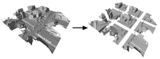
Figure 3.
Dividing mesh into nine blocks.
A plane may be split into multiple parts in this method, and the generated planes would be merged. The merging of adjacent plane is realized by the dual graph. The dual graph is defined by mapping every plane to a node in the dual graph, and the two dual nodes are connected by an edge if the corresponding plane is adjacent in the mesh. An edge collapse in this graph will merge two nodes into one, which corresponds to grouping their associated faces into a single plane. Figure 4 illustrates an example. In the dual graph, underlying planes are shown in a different color. Figure 4a is a mesh where each dual node corresponds to a plane. Similar to edge collapse [53], a new vertex is created after each contraction. The edge is contracted on the top of the graph, and its dual nodes are merged. After a collapse, the two regions are merged to produce a single region, as shown in Figure 4b.
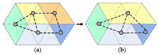
Figure 4.
Merge plane. Each color represents a plane. (a) The correspondence between the plane and dual graphs. (b) An edge in the dual graph is collapsed, and the two planes corresponding to the edge endpoints are merged into a new plane.
For this study, a simple greedy approach is adopted in the merging process, similar to the existing mesh decimation algorithm. Each edge is assigned a price-value, and the edge with the least price-value is collapsed in each iteration. The result of the merge should satisfy two objectives: (1) The effect on the approximate error of the plane should be minimized after merging, and (2) the merged region with a more regular shape should be prioritized. Thus, the price-value of the edge is defined by:
where the price-value is composed of two components: and . The first term in Equation (5) corresponds to the first objective, which measures the change of error before and after the plane merge. It is defined as:
where and are the errors of planes and , respectively, and is the error of the new plane after plane and are merged. The plane error is the sum of the error of each face in the plane. The value of is greater than or . The larger the value of , the merged result less approximate to a plane, and will increase.
The second term in Equation (5) corresponds to the second objective, which measures the changes of shape. It is defined as:
where and are the shape factors of planes , , respectively, is the shape factor of the merging planes and . is the ratio of the squared perimeter to the squared perimeter of a circle with area . In the ideal case , the plane is a circle. The larger value of corresponds to the more irregular plane. To quickly calculate the shape factor, the area and the perimeter of the plane have to be determined. The area is easy to calculate, which is simply the sum of the area of the constituent planes. For the perimeter, the values are not additive. In each plane, the perimeter information is recorded in a dual node. When two planes are merged, the perimeter of the resulting plane is the sum of the perimeters of the constituent planes minus twice the length of the boundary separating them.
Figure 5 shows the changes of the merged result after the shape factor is added. Each color represents a plane in each result. In Figure 5b, only the plane error is considered, and the merged result is irregular. In Figure 5c, the merged result shows a more regular form than Figure 5b, after the shape factor is added.
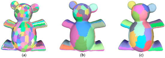
Figure 5.
Merging results from different factors. (a) Variational Shape Approximation (VSA) mesh segmentation; (b) only with approximation error; (c) combined shape factors.
The geometry attribute of the mesh is not altered by this merging algorithm. Each vertex remains in its original position, and the connectivity of faces is unchanged. Only the number of nodes in the graph is constantly decreasing. When the minimum price–value of the edge reaches the set threshold, the merging algorithm stops collapsing, and the merge is completed.
4.2. Texture Chart Generation Method with the Mesh Planar-Structure Information
A texture chart is a set of topologically adjacent faces with the same image label. The result of the texture chart generation depends on the selected image label for each face. Typically, there is more than one visual image for each face, and choosing an optimal visual image from all candidate images for each face is essentially a multi-label graph cut optimization problem. As shown in Figure 6, we constructed an undirected weighted graph of mesh, where the number of nodes and the number of faces is equal. Each face in the surface model is regarded as a node in graph , and the edges between nodes represent the adjacent relationship between faces. There are k terminal nodes, with each corresponding to an image in the graph. The edges connecting the terminal node and common nodes are t-link, which means that the face is visible on this image. Moreover, the edges connecting the common nodes are n-link, indicating an adjacent relationship between the two faces. When considering these edges as pipelines, finding the max flow from one terminal to another terminal is a Max Flow problem. Liu et al. [54] pointed out that when the n-link edges are located in the max flow and separate the terminal nodes, the cut of these edges is the minimum cut. Therefore, this becomes a MaxFlow cut and MinCut problem.
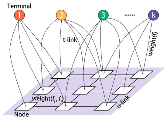
Figure 6.
Our multi-labeled graph.
The graph cut energy function is the mathematical expression of the actual problem and provides the bridge between the graph cut theory and specific problems. The weights of the edges are determined by the MRF energy function in the graph. Compared with the original MRF energy function, the mesh model’s structural information (plane) is introduced and integrated with the visual information of the 3D triangle face on the image as the constraint condition of the smoothness term’s value. Our improved energy function formula is as follows:
The data item indicates the possibility of node selecting the image with the label . The visual quality of the face on the image is used as the value of the data item. is the smoothness term, which affects the image selection of the adjacent faces. To ensure that the faces do not deviate too far from the original segmentation plane during the optimization process, this study also takes the angle between each pair of adjacent nodes , the charts that the nodes belong to, and the selected image, as three factors. Different weights to were given for the six different cases, as presented in Table 1.

Table 1.
The value of .
Texture mapping should prioritize image quality. When the adjacent faces are on the same chart and can be captured by the same image (), the value of the smoothness term is 0 (). On the contrary, when the adjacent faces are neither in the same plane nor captured by the same image, the value of the smoothness term is infinite (). If the dihedral angle is greater than the threshold (30 degrees in this study) (), the visual quality on the same image cannot be assured, and the smoothness term is also infinite (). The above four cases have fixed parameters, and the optimization effect of the energy function depends on the settings of and . The optimization of texture charts would eventually affect the display effect. The display effect can be evaluated by the texture quality of each face and the number of texture charts. In this study, we propose the use of texture clarity to evaluate the optimized texture quality. Formula is defined as follows:
where is the visual clarity for each face on the specified image after optimization, and is the number of texture charts after optimization. As shown in Figure 7, the influence of and on the optimization effect is tested separately by the control variable method. When , , the texture visual quality increases rapidly, and the number of texture charts continuously decreases. When , the optimization effect begins to converge. When , , the texture clarity declines slowly, and the number of texture charts gradually increases. The change is not obvious. When , it would be more advisable to reduce the number of texture charts and improve the display effect of textures. In this study, we used and as the smoothness term’s value.
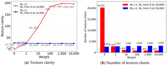
Figure 7.
The influence of , on optimization results: (a) fix the values of ,, respectively, the changes of texture clarity; (b) fix the values of ,, respectively, the change of texture charts’ number.
Moreover, the value of the data item needs to be normalized. This is because the fluctuating value of the energy is supposed to be in the same order of magnitude in the graph cut problem; otherwise, the expected result and the abstract model will intensify the difference. Here, we adopted the value of 99.5% for the normalization.
For this study, we used the - optimization algorithm to solve the energy function. This algorithm can split the initially labeled data set and transform the multidimensional undirected graph into a two-dimensional simple undirected single graph, thereby avoiding the uncertainty of t-link and n-link capacity [55]. The basic idea behind this algorithm is that by exchanging α and β label sets, a new label set can be formed by assuming that there are two labels and in the known label set and the segmented set . To ensure that the cut in the Graph-Cuts is smaller than the original ones in the new label set, the algorithm is iterated until the minimum cut in the Graph-Cuts appears. The label set that splits the set can be expressed as , where is the definitional domain of the label set, and is the subset of label in the set . The - is applied to a given set of labels and , indicating the exchange of and and forms a new segmented set . The remaining set of and , which is not contained in label , remains unchanged.
4.3. Texture Charts Boundary Smoothing
The texture chart generated according to the graph-cut would result in a jagged boundary, increasing the sampling error of the chart’s boundary seam. A smoothing method needs to be adopted to shorten the boundary length. For this study, two boundary smoothing principles are proposed when the face is visible in the selected image of the adjacent texture chart. These principles are implemented as follows:
- Quantity priority principle: Traverse all adjacent charts of the face, and count the number of texture charts. If two or more faces belong to the same texture chart, the current face is also added to this largest texture chart.
- The longest side principle: Count the length of the three sides of the face if the texture charts to which the adjacent faces belong are different. Sort the edges in order from large to small, and the current face is added to the texture chart corresponding to the longest edge.
Figure 8 presents the results of boundary smoothing, where the different texture charts are represented by different colors. In the image, there are only two texture blocks around the triangles and . According to the principle of number dominance, and are smoothed to the pink and green charts, respectively. For the triangle surface , three texture charts surround the surface, which, according to the longest side principle, is optimized into the green texture chart.
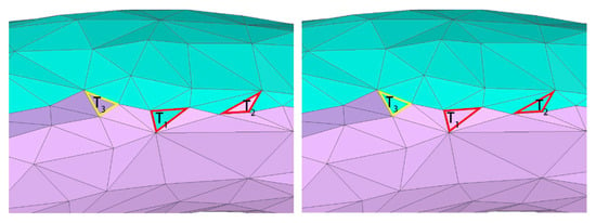
Figure 8.
Boundary smoothing. Left: un-smoothed boundary; Right: smoothed boundary.
5. Experiments and Analysis
To verify the effectiveness of our algorithm, we utilized the model using different data types and images from different regions with varying numbers and angles. The experiment content includes two parts: qualitative assessment and quantitative evaluation. We compared the experimental results with the open-source program OpenMVS, which provides a complete set of processes to recover the full surface of the scene from being reconstructed. OpenMVS is an open-source method that is convenient for others to learn and improve and can be easily transplanted to other application scenarios. This experiment is modified based on OpenMVS, and the theoretical content of this study is implemented by replacing the code of the texture chart generation.
The experimental models and images are divided into three data sets. The image details are specified in Table 2. Figure 9 shows the 3D models without texture. The experimental models were all generated from the corresponding images using OpenMVS. Among them, Church is a close-range model (building gate), Villa is a small-scale model (a building), and City is a large-scale model (the entire city). These models cover the major reconstruction types, and it is of universal significance to texturing them. The computer environment used in the experiments was a Win10 64-bit operating system, with 64G computer memory, Intel Core i7 (3.6 GHz, four cores, and eight threads). The test program was written in the C++ language, and the model display software was MeshLab [56].

Table 2.
Experimental data information.

Figure 9.
3D models without texture.
5.1. Qualitative Assessment Experiments
5.1.1. Qualitative Comparison of the Number of Texture Charts
To verify the effect of our proposed approach, our algorithm and the OpenMVS method were used to generate the texture charts. Our algorithm contains two results planar structural segmentation and generated texture chart. Planar structural segmentation results were produced using the methodology discussed in Section 4.1. The method used in generating texture chart results is discussed in Section 4.2 and Section 4.3. The default value of 9 was used for the number of blocks.
The results are presented in Figure 10, Figure 11 and Figure 12. In each method, different colors represent different texture charts. The number of texture charts generated by our algorithm is less than the number generated by OpenMVS.
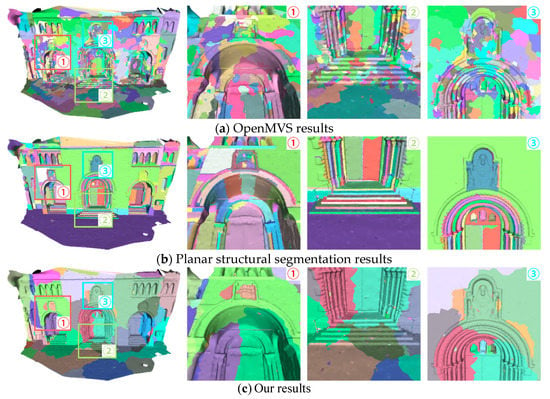
Figure 10.
The texture charts with different methods for the Church. In each method, different colors represent different texture charts; (a) OpenMVS results; (b) planar structural segmentation results; (c) our results.
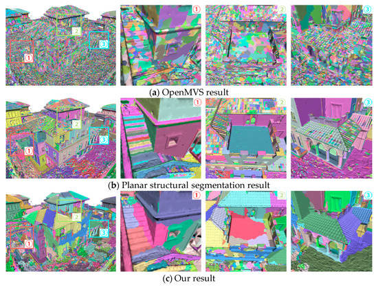
Figure 11.
The texture charts with different methods for Villa. In each method, different colors represent different texture charts; (a) OpenMVS results; (b) planar structural segmentation results; (c) our results.
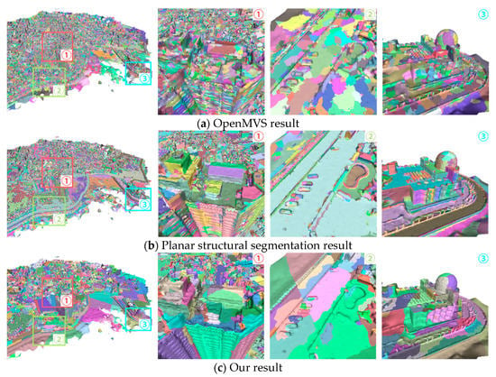
Figure 12.
The texture charts with different methods for City. In each method, different colors represent different texture charts; (a) OpenMVS results; (b) planar structural segmentation results; (c) our results.
From the local zoom view, the boundaries of planer structural segmentation results are mostly located in high curvature regions of the models, such as wall corners (Church: region 1 of Figure 10; Villa: region 1 and 2 of Figure 11; City: region 1 and 3 of Figure 12) and staircase edges (Church: region 2 of Figure 10; Villa: region 1 of Figure 11), and can represent all the planes of the model well. For the results of our method, the texture charts differed significantly. In the plane region, the texture charts were further segmented by MRF energy function. In the non-planar region, A large number of planes are merged. For example, in region 3 of Figure 11, due to the undulations of roof tiles, the OpenMVS and plane segmentation results showed large numbers of fragments. In the results using our MRF energy function, the number of texture charts is significantly declined. The same observation can be made for the observatory’s dome in the City (region 1 and 3 of Figure 12).
5.1.2. Qualitative Comparison of Texture Reconstruction Results
The texture charts produced in Section 5.1.1 were used for texture reconstruction. The texture reconstruction result of our algorithm and OpenMVS is visually shown in Figure 13, Figure 14 and Figure 15. As shown by comparing the overall display effects, the texture reconstruction effects generated by the two methods are relatively similar. However, the overall effect generated by OpenMVS is darker, and the model texture resolution is lower, which is due to the large number of generated texture charts. From the local zoom view, OpenMVS generated a large number of texture charts that resulted in problems, such as color inconsistency, mapping errors, and seam lines. For example, errors and inconsistencies can be found in the generated images displaying the wall corner of the Church (region 1 and 3 of Figure 13), the roof of the Villa (region 1 of Figure 14), and the parking area of the City (region 2 of Figure 15). In contrast, our algorithm significantly reduced or even eliminated some of these problems. Using our proposed approach, more texture information was retained, and the problem of miscutting and large color discontinuity between texture charts had been resolved.
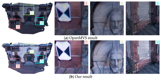
Figure 13.
The texture display effect of two methods for Church. (a) OpenMVS result; (b) our result.
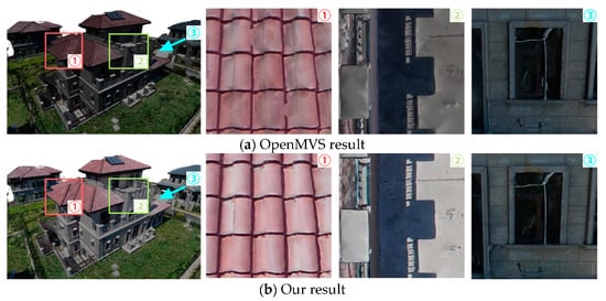
Figure 14.
The texture display effect of two methods for Villa. (a) OpenMVS result; (b) our result.
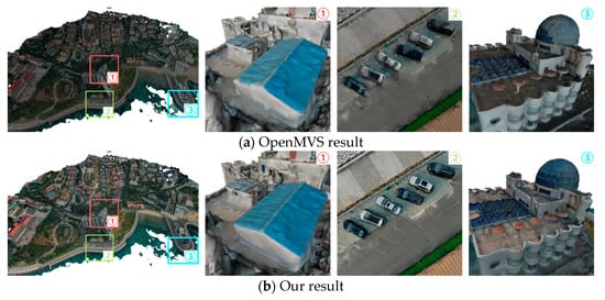
Figure 15.
The texture display effect of two methods for City. (a) OpenMVS result; (b) our result.
5.2. Quantitative Evaluation Experiments
5.2.1. Efficiency Comparison with OpenMVS Texture Reconstruction Algorithm
In Section 4.1.3, we showed that our algorithm could improve the efficiency of texture chart segmentation through the model split. In both the OpenMVS and our proposed algorithm, the color adjustment algorithm by Lempitsky et al. [28] is adopted, which separately adjusts the color of the texture image corresponding to each pair of adjacent texture charts. The reduction in the number of texture charts would significantly result in less time required by the color adjustment algorithm.
To verify if our method can improve the efficiency in plane segmentation, we compared the time consumed with original VSA algorithm. As shown in the summary of results presented in Table 3, our fully automatic plane segmentation algorithm consumed less processing time than the original VSA algorithm. The highest efficiency improvement was found in the processing of the City model.

Table 3.
Efficiency comparison of VSA and our method.
This experiment simplifies the mesh model to different data quantities to test the texture reconstruction efficiency of our method. In Figure 16, the texture reconstruction running time from the proposed approach is compared with the OpenMVS method for the three models. The horizontal axis is the number of triangles of the simplified model, and the vertical axis is the running time. The bar with a red border is the statistical results of running time using the OpenMVS method, and the bar with green borders is the statistical results from our proposed approach. Overall, the total time for texture reconstruction generated in our method was shorter than in the OpenMVS. With the number of faces increased, our proposed algorithm was able to shorten the running time. In terms of image scoring, the two methods registered similar times due to having similar image scoring strategies. Since our proposed approach uses parallel computing, the segmentation efficiency is better than the OpenMVS. In terms of color adjustment, owing to cutting down the number of texture charts, the running time decreased when the proposed algorithm was used. With the number of faces increased, the efficiency of color adjustment significantly improved. The results suggest that the efficiency improvements of our method are more significant for the texture mapping of larger scenes.

Figure 16.
Comparison of texture reconstruction efficiency (unit of the running time is second). (a) Church running times; (b) villa running times; (c) city running times.
5.2.2. Quantitative Comparison of the Number of Texture Charts
The number of texture charts is a quantitative evaluation index that is currently used more frequently [57,58]. Figure 17 presents the statistics of the number of texture charts generated by OpenMVS and our proposed algorithm. Different methods are marked with different colors. As shown in Figure 17, the texture charts generated by our proposed algorithm have been significantly reduced compared with the OpenMVS technique. Besides, the number of texture charts generated by our method is smaller than the number of model planes.

Figure 17.
Changes in the number of texture charts generated by our algorithm and OpenMVS. (a) Church results; (b) villa results; (c) city results.
5.2.3. Quantitative Comparison of the Total Length of Texture Seam-Line
The seam-line is the common boundary edge between two adjacent texture charts. Texture color discontinuities are prone to appear at the seam-line. The longer the seam-line, the more the color errors. Calculating the length of the seam-line can effectively measure the texture discontinuity problem of texture reconstruction results. Our algorithm can reduce the length of the seam-line by reducing the number of texture charts. To verify the improvement in the reconstruction effect, we analyzed the seam-line length. The statistical results of the seam-line length in Figure 18. The seam-line length of the texture chart generated by our method is significantly smaller than the boundary length generated by OpenMVS.
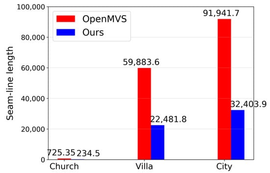
Figure 18.
Seam-line length of OpenMVS and our algorithm.
5.2.4. Quantitative Comparison of Texture Clarity
Shan et al. [59] mentioned that the resolution (clarity) of texture is an important indicator of the true degree of authenticity of texture reconstruction. However, if only the clarity is used, the method of directly specifying the sharpest image for each triangle face will get the highest score. It is unreasonable because the number of texture charts also needs to be considered. Therefore, this paper uses the average texture clarity of each texture chart (formula 9) as the evaluation index. The statistical results of texture clarity are shown in Figure 19. The texture clarity generated by our algorithm is gradually improved with the amount of data increasing, while the texture clarity generated by OpenMVS is gradually decreasing. This suggests that our proposed algorithm could improve the texture reconstruction effect.
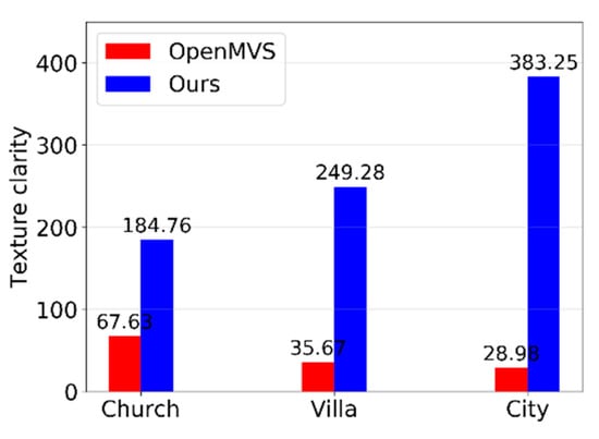
Figure 19.
Texture clarity comparison of OpenMVS and our algorithm.
5.3. Discussion
Based on experiments on three typical sets of UAV data with different reconstruction range, the experimental conclusions are as follows: (1) the improved OpenMVS texture chart generation method proposed in this paper was suitable for scenes with different reconstruction ranges. Compared with the original OpenMVS texture chart generation method, our method reduced the number of texture charts, and exerted a profound improvement on the miscuts and color differences between texture charts. The texture reconstruction results were more natural. (2) Due to the improved VSA plane segmentation algorithm adopted multithread parallel processing, compared with the original VSA algorithm, the proposed algorithm highly boosted the extraction efficiency of mesh model planar structure features. To a certain extent, it also improved the efficiency of OpenMVS texture reconstruction algorithm. Compared with the original OpenMVS texture chart generation method, the proposed method greatly reduced the number of texture charts, shortened the total length of the seam-line, and significantly improved the average texture chart clarity.
From the experiments, however, we also found that there is still room for improvement in our method. Parallel computing requires the merging of texture charts, which would still require the use of considerable time. For future studies, the algorithm can be further improved to achieve a more detailed and faster 3D texture reconstruction.
6. Conclusions
Texture reconstruction is a hot topic in the field of digital photogrammetry and computer vision. Given insufficient consideration of the smoothness term in the MRF energy function constructed by existing 3D texture reconstruction methods, the generated texture chart results still had considerable fragment problems (which will result in serious local miscuts and color discontinuity between texture charts and reduce the execution efficiency), and jaggy boundaries between texture charts. This study fully utilized the planar structure information of the mesh model and the visual information of the 3D triangle face on the image and proposed an improved, faster, and high-quality texture chart generation method based on the OpenMVS texture chart generation algorithm. The main methodology is as follows: first, the visual quality of different visual images is scored for each triangle face. The plane structural features of the mesh model are extracted, and the processing flow is partitioned into three parts: (1) splitting mesh into blocks; (2) automatic segmentation of all planes in each block; and (3) merging of planes that are on the same plane between adjacent blocks. Finally, the plane structure information of the model is integrated into the MRF energy function. The graph cut is used to minimize the energy function to obtain the texture charts, and the boundary of the texture chart is smoothed.
In general, we proposed a novel OpenMVS-based texture reconstruction method based on the fully automatic plane segmentation algorithm using the improved variational shape approximation framework for 3D mesh models. Our method solves the problem of the existing MRF energy function, wherein it only considers the selection of the image label of the adjacent triangle face for the smoothness term and ignores the planar-structure information of the model. Compared with the original OpenMVS texture chart generation method, this study’s method achieved the following three goals: (1) improving the operating efficiency of the OpenMVS texture chart generation method to a certain extent; (2) reducing the number of texture charts (it helps ameliorate the problem by miscuts and large color discontinuity between texture charts); (3) to a certain extent, minimizing the sampling error of the boundary seam-line of texture charts.
Author Contributions
S.L., X.X., and B.G. proposed the idea and wrote the manuscript; S.L., X.X., and L.Z. designed and performed experiments; X.X. and S.L. revised the manuscript and added several experiments to improve the quality of the manuscript. All authors have read and agreed to the published version of the manuscript.
Funding
This research was funded by the National Natural Science Foundation of China (Grant Nos. 91638203, 91738302), Fundamental Research Funds for the Central Universities of China (Grant No. 2042019kf0002), China Scholarship Council (Grant No. 201606270125), the Science and Technology Program of Southwest China Research Institute of Electronic Equipment (Grant No. JS20200500114), the Key Laboratory of Urban Land Resources Monitoring and Simulation, Ministry of Land and Resources (Grant No. KF-2018-03-052), the Science and Technology Program of Guangzhou, China (Grant No. 2017010160173) and LIESMARS Special Research Funding.
Acknowledgments
We would like to thank the reviewers for their detailed comments and nice suggestions, which greatly improved the manuscript. We also thank Zhe Peng for conceiving and designing the experiments. This work is partly supported by Wuhan Xuntu Technology Co. Ltd. We are thankful for Stephen C. McClure for providing us English editing of the manuscript freely.
Conflicts of Interest
The authors declare no conflict of interest.
References
- Xie, H.; Yao, H.; Sun, X.; Zhou, S.; Zhang, S. Pix2vox: Context-aware 3d reconstruction from single and multi-view images. In Proceedings of the IEEE International Conference on Computer Vision, Seoul, Korea, 27 October–2 November 2019; pp. 2690–2698. [Google Scholar]
- Jing-Xue, Y.; Qiang, Z.; Wei-Xi, Y. A dense matching algorithm of multi-view image based on the integrated multiple matching primitives. Acta Geod. Cartogr. Sin. 2013, 42, 691. [Google Scholar]
- Seitz, S.M.; Curless, B.; Diebel, J.; Scharstein, D.; Szeliski, R. A comparison and evaluation of multi-view stereo reconstruction algorithms. In Proceedings of the 2006 IEEE Computer Society Conference on Computer Vision and Pattern Recognition (CVPR’06), New York, NY, USA, 17–22 June 2006; pp. 519–528. [Google Scholar]
- Rouhani, M.; Lafarge, F.; Alliez, P. Semantic segmentation of 3D textured meshes for urban scene analysis. ISPRS J. Photogramm. Remote Sens. 2017, 123, 124–139. [Google Scholar] [CrossRef]
- Pepe, M.; Fregonese, L.; Crocetto, N. Use of SfM-MVS approach to nadir and oblique images generated throught aerial cameras to build 2.5 D map and 3D models in urban areas. Geocarto Int. 2019, 1–22. [Google Scholar] [CrossRef]
- Purnomo, B.; Cohen, J.D.; Kumar, S. Seamless texture atlases. In Proceedings of the 2004 Eurographics/ACM SIGGRAPH Symposium on Geometry Processing, Nice, France, 8–10 July 2004; pp. 65–74. [Google Scholar]
- Bi, S.; Kalantari, N.K.; Ramamoorthi, R. Patch-based optimization for image-based texture mapping. ACM Trans. Graph. 2017, 36, 106:1–106:11. [Google Scholar] [CrossRef]
- Inzerillo, L.; Di Paola, F.; Alogna, Y. High quality texture mapping process aimed at the optimization of 3d structured light models. Int. Arch. Photogramm. Remote Sens. Spat. Inf. Sci. 2019, 389–396. [Google Scholar] [CrossRef]
- Lai, J.-Y.; Wu, T.-C.; Phothong, W.; Wang, D.W.; Liao, C.-Y.; Lee, J.-Y. A high-resolution texture mapping technique for 3D textured model. Appl. Sci. 2018, 8, 2228. [Google Scholar] [CrossRef]
- Xu, L.; Li, E.; Li, J.; Chen, Y.; Zhang, Y. A general texture mapping framework for image-based 3D modeling. In Proceedings of the 2010 IEEE International Conference on Image Processing, Hong Kong, China, 12–15 September 2010; pp. 2713–2716. [Google Scholar]
- Schönberger, J.L.; Zheng, E.; Frahm, J.-M.; Pollefeys, M. Pixelwise view selection for unstructured multi-view stereo. In Proceedings of the European Conference on Computer Vision, Amsterdam, The Netherlands, 11–14 October 2016; pp. 501–518. [Google Scholar]
- Fuhrmann, S.; Langguth, F.; Moehrle, N.; Waechter, M.; Goesele, M. MVE—An image-based reconstruction environment. Comput. Graph. 2015, 53, 44–53. [Google Scholar] [CrossRef]
- Hepp, B.; Nießner, M.; Hilliges, O. Plan3d: Viewpoint and trajectory optimization for aerial multi-view stereo reconstruction. ACM Trans. Graph. TOG 2018, 38, 1–17. [Google Scholar] [CrossRef]
- Iizuka, S.; Simo-Serra, E.; Ishikawa, H. Let there be color! Joint end-to-end learning of global and local image priors for automatic image colorization with simultaneous classification. ACM Trans. Graph. ToG 2016, 35, 1–11. [Google Scholar] [CrossRef]
- Yeo, D.; Lee, C.-O. Variational shape prior segmentation with an initial curve based on image registration technique. Image Vis. Comput. 2020, 94, 103865. [Google Scholar] [CrossRef]
- Cohen-Steiner, D.; Alliez, P.; Desbrun, M. Variational shape approximation. In ACM SIGGRAPH 2004 Papers; Association for Computing Machinery: New York, NY, USA, 2004; pp. 905–914. [Google Scholar]
- Yan, D.-M.; Wang, W.; Liu, Y.; Yang, Z. Variational mesh segmentation via quadric surface fitting. Comput. Aided Des. 2012, 44, 1072–1082. [Google Scholar] [CrossRef]
- Wu, N.; Zhang, D.; Deng, Z.; Jin, X. Variational Mannequin Approximation Using Spheres and Capsules. IEEE Access 2018, 6, 25921–25929. [Google Scholar] [CrossRef]
- Morigi, S.; Huska, M. Sparsity-inducing variational shape partitioning. Electron. Trans. Numer. Anal. 2017, 46, 36–54. [Google Scholar]
- Cernea, D. OpenMVS: Open Multiple View Stereovision. Available online: https://github.com/cdcseacave/openMVS/ (accessed on 18 November 2020).
- Callieri, M.; Cignoni, P.; Corsini, M.; Scopigno, R. Masked photo blending: Mapping dense photographic data set on high-resolution sampled 3D models. Comput. Graph. 2008, 32, 464–473. [Google Scholar] [CrossRef]
- Hoegner, L.; Stilla, U. Automatic 3D reconstruction and texture extraction for 3D building models from thermal infrared image sequences. Quant. InfraRed Thermogr. 2016. [Google Scholar] [CrossRef]
- Liu, L.; Ye, C.; Ni, R.; Fu, X.-M. Progressive parameterizations. ACM Trans. Graph. TOG 2018, 37, 1–12. [Google Scholar] [CrossRef]
- Li, S.; Luo, Z.; Zhen, M.; Yao, Y.; Shen, T.; Fang, T.; Quan, L. Cross-atlas convolution for parameterization invariant learning on textured mesh surface. In Proceedings of the IEEE Conference on Computer Vision and Pattern Recognition, Long Beach, CA, USA, 15–21 June 2019; pp. 6143–6152. [Google Scholar]
- Zhao, H.; Li, X.; Ge, H.; Lei, N.; Zhang, M.; Wang, X.; Gu, X. Conformal mesh parameterization using discrete Calabi flow. Comput. Aided Geom. Des. 2018, 63, 96–108. [Google Scholar] [CrossRef]
- Lee, J.; Yang, B. Developing an optimized texture mapping for photorealistic 3D buildings. Trans. GIS 2019, 23, 1–21. [Google Scholar] [CrossRef]
- Yin, Y.; Chen, H.; Meng, X.; Yang, X.; Peng, X. Texture mapping based on photogrammetric reconstruction of the coded markers. Appl. Opt. 2019, 58, A48–A54. [Google Scholar] [CrossRef]
- Lempitsky, V.; Ivanov, D. Seamless mosaicing of image-based texture maps. In Proceedings of the 2007 IEEE Conference on Computer Vision and Pattern Recognition, Minneapolis, MN, USA, 17–22 June 2007; pp. 1–6. [Google Scholar]
- Fu, Y.; Yan, Q.; Yang, L.; Liao, J.; Xiao, C. Texture mapping for 3d reconstruction with rgb-d sensor. In Proceedings of the IEEE Conference on Computer Vision and Pattern Recognition, Salt Lake City, UT, USA, 18–22 June 2018; pp. 4645–4653. [Google Scholar]
- Li, W.; Gong, H.; Yang, R. Fast texture mapping adjustment via local/global optimization. IEEE Trans. Vis. Comput. Graph. 2018, 25, 2296–2303. [Google Scholar] [CrossRef]
- Yang, Y.; Zhang, Y. A high-realistic texture mapping algorithm based on image sequences. In Proceedings of the 2018 26th International Conference on Geoinformatics, Kunming, China, 28–30 June 2018; pp. 1–8. [Google Scholar]
- Jagannathan, A.; Miller, E.L. Three-dimensional surface mesh segmentation using curvedness-based region growing approach. IEEE Trans. Pattern Anal. Mach. Intell. 2007, 29, 2195–2204. [Google Scholar] [CrossRef] [PubMed]
- Vieira, M.; Shimada, K. Surface mesh segmentation and smooth surface extraction through region growing. Comput. Aided Geom. Des. 2005, 22, 771–792. [Google Scholar] [CrossRef]
- Liu, S.; Ferguson, Z.; Jacobson, A.; Gingold, Y.I. Seamless: Seam erasure and seam-aware decoupling of shape from mesh resolution. ACM Trans. Graph. 2017, 36, 216:1–216:15. [Google Scholar] [CrossRef]
- Jiao, X.; Wu, T.; Qin, X. Mesh segmentation by combining mesh saliency with spectral clustering. J. Comput. Appl. Math. 2018, 329, 134–146. [Google Scholar] [CrossRef]
- Lee, J.; Kim, S.; Kim, S.-J. Mesh segmentation based on curvatures using the GPU. Multimed. Tools Appl. 2015, 74, 3401–3412. [Google Scholar] [CrossRef]
- He, C.; Wang, C. A survey on segmentation of 3D models. Wirel. Pers. Commun. 2018, 102, 3835–3842. [Google Scholar] [CrossRef]
- Attene, M.; Falcidieno, B.; Spagnuolo, M. Hierarchical mesh segmentation based on fitting primitives. Vis. Comput. 2006, 22, 181–193. [Google Scholar] [CrossRef]
- Marinov, M.; Kobbelt, L. Automatic generation of structure preserving multiresolution models. In Proceedings of the Computer Graphics Forum, Amsterdam, The Netherlands, 18–20 May 2005; pp. 479–486. [Google Scholar]
- Khattab, D.; Ebeid, H.M.; Hussein, A.S.; Tolba, M.F. 3D Mesh Segmentation Based on Unsupervised Clustering. In Proceedings of the International Conference on Advanced Intelligent Systems and Informatics, Cairo, Egypt, 24–26 October 2016; pp. 598–607. [Google Scholar]
- Garland, M.; Willmott, A.; Heckbert, P.S. Hierarchical face clustering on polygonal surfaces. In Proceedings of the 2001 Symposium on Interactive 3D Graphics, Chapel Hill, NC, USA, 26–29 March 2001; pp. 49–58. [Google Scholar]
- Wang, H.; Lu, T.; Au, O.K.-C.; Tai, C.-L. Spectral 3D mesh segmentation with a novel single segmentation field. Graph. Models 2014, 76, 440–456. [Google Scholar] [CrossRef]
- Cheng, S.-C.; Kuo, C.-T.; Wu, D.-C. A novel 3D mesh compression using mesh segmentation with multiple principal plane analysis. Pattern Recognit. 2010, 43, 267–279. [Google Scholar] [CrossRef]
- Kaiser, A.; Ybanez Zepeda, J.A.; Boubekeur, T. A survey of simple geometric primitives detection methods for captured 3d data. In Proceedings of the Computer Graphics Forum, Brno, Czech Republic, 4–8 June 2018; pp. 167–196. [Google Scholar]
- Yi, B.; Liu, Z.; Tan, J.; Cheng, F.; Duan, G.; Liu, L. Shape recognition of CAD models via iterative slippage analysis. Comput. Aided Des. 2014, 55, 13–25. [Google Scholar] [CrossRef]
- Wang, J.; Yu, Z. Surface feature based mesh segmentation. Comput. Graph. 2011, 35, 661–667. [Google Scholar] [CrossRef]
- Sun, C.-Y.; Zou, Q.-F.; Tong, X.; Liu, Y. Learning adaptive hierarchical cuboid abstractions of 3d shape collections. ACM Trans. Graph. TOG 2019, 38, 1–13. [Google Scholar] [CrossRef]
- Quan, W.; Guo, J.; Zhang, X.; Dongming, Y.; Yan, D. Improved quadric surfaces recognition from scanned mechanical models. CADDM 2016, 26, 9–19. [Google Scholar]
- Simari, P.D.; Singh, K. Extraction and remeshing of ellipsoidal representations from mesh data. In Proceedings of the Graphics Interface, Victoria, BC, Canada, 9–11 May 2005; pp. 161–168. [Google Scholar]
- Wu, J.; Kobbelt, L. Structure Recovery via Hybrid Variational Surface Approximation. In Proceedings of the Comput. Graph. Forum, Amsterdam, The Netherlands, 18–20 May 2005; pp. 277–284. [Google Scholar]
- Thul, D.; Ladický, L.U.; Jeong, S.; Pollefeys, M. Approximate convex decomposition and transfer for animated meshes. ACM Trans. Graph. TOG 2018, 37, 1–10. [Google Scholar] [CrossRef]
- Waechter, M.; Moehrle, N.; Goesele, M. Let there be color! Large-scale texturing of 3D reconstructions. In Proceedings of the European Conference on Computer Vision, Zurich, Switzerland, 6–12 September 2014; pp. 836–850. [Google Scholar]
- Salinas, D.; Lafarge, F.; Alliez, P. Structure-aware mesh decimation. In Proceedings of the Computer Graphics Forum, Graz, Austria, 6–8 July 2015; pp. 211–227. [Google Scholar]
- Liu, L.; Sheng, Y.; Zhang, G.; Ugail, H. Graph cut based mesh segmentation using feature points and geodesic distance. In Proceedings of the 2015 International Conference on Cyberworlds (CW), Visby, Sweden, 7–9 October 2015; pp. 115–120. [Google Scholar]
- Schmidt, M.; Alahari, K. Generalized fast approximate energy minimization via graph cuts: Alpha-expansion beta-shrink moves. arXiv 2011, arXiv:Preprint/1108.5710. [Google Scholar]
- Cignoni, P.; Callieri, M.; Corsini, M.; Dellepiane, M.; Ganovelli, F.; Ranzuglia, G. Meshlab: An open-source mesh processing tool. In Proceedings of the Eurographics Italian Chapter Conference, Salerno, Italy, 2–4 July 2008; pp. 129–136. [Google Scholar]
- Schuster, K.; Trettner, P.; Schmitz, P.; Kobbelt, L. A Three-Level Approach to Texture Mapping and Synthesis on 3D Surfaces. Proc. ACM Comput. Graph. Interact. Tech. 2020, 3, 1–19. [Google Scholar]
- Velho, L.; Sossai, J., Jr. Projective texture atlas construction for 3D photography. Vis. Comput. 2007, 23, 621–629. [Google Scholar] [CrossRef]
- Shan, Q.; Adams, R.; Curless, B.; Furukawa, Y.; Seitz, S.M. The visual turing test for scene reconstruction. In Proceedings of the 2013 International Conference on 3D Vision-3DV 2013, Seattle, WA, USA, 29 June–1 July 2013; pp. 25–32. [Google Scholar]
Publisher’s Note: MDPI stays neutral with regard to jurisdictional claims in published maps and institutional affiliations. |
© 2020 by the authors. Licensee MDPI, Basel, Switzerland. This article is an open access article distributed under the terms and conditions of the Creative Commons Attribution (CC BY) license (http://creativecommons.org/licenses/by/4.0/).