The New Landsat Collection-2 Digital Elevation Model

Abstract

The Landsat Collection-2 distribution introduces a new global Digital Elevation Model (DEM) for scene orthorectification. The new global DEM is a composite of the latest and most accurate freely available DEM sources and will include reprocessed Shuttle Radar Topographic Mission (SRTM) data (called NASADEM), high-resolution stereo optical data (ArcticDEM), a new National Elevation Dataset (NED) and various publicly available national datasets including the Canadian Digital Elevation Model (CDEM) and DEMs for Sweden, Norway and Finland (SNF). The new DEM will be available world-wide with few exceptions. It is anticipated that the transition from the Collection-1 DEM at 3 arcsecond to the new DEM will be seamless because processing methods to maintain a seamless transition were employed, void filling techniques were used, where persistent gaps were found, and the pixel spacing is the same between the two collections. Improvements to the vertical accuracy were realized by differencing accuracies of other elevation datasets to the new DEM. The greatest improvement occurred where ArcticDEM data were used, where an improvement of 35 m was measured. By using theses improved vertical values in a line of sight algorithm, horizontal improvements were noted in some of the most mountainous regions over multiple 30-m Landsat pixels. This new DEM will be used to process all of the scenes from Landsat 1-8 in Collection-2 processing and will be made available to the public by the end of 2020.

1. Introduction

The U.S. Geological Survey (USGS) Earth Resources Observation and Science (EROS) Center processes and delivers Landsat terrain-corrected products to the public through the implementation of Collections. The strategy of Collections requires reprocessing of the entire Landsat archive on a periodic basis to update the radiometric and geometric accuracies of the standard products using improved reference data and algorithms. The first implementation of the Collections processing, referred to as Collection-1, was released in 2016. The Landsat products in Collection-1 are corrected for terrain elevation effects using the Global Land Survey Digital Elevation Model (GLSDEM), which is a mosaic of multiple sources of Digital Elevation Models (DEM), developed initially by MacDonald, Dettwiler and Associates Federal (subsidiary of Maxar Technologies) in 2007 and later updated by the Calibration and Validation Team (CalVal) at USGS EROS. The GLSDEM used the USGS National Elevation Dataset (NED) over the United States and Alaska, whereas Canadian Digital Elevation Data (CDED) were used over Canada. North of 60 degrees north latitude, a combination of Digital Terrain Elevation Data (DTED) level-1 and Global Multiresolution Terrain Elevation Data (GMTED) 2010 data were used. For the rest of the landmass, the Consultative Group on International Agricultural Research (CGIAR) “hole-filled” Shuttle Radar Topographic Mission (SRTM) data were used. Prior to Collection-1, the USGS updated DEM tiles with large artifacts using improved elevation datasets, which generated a consistent global DEM at 3 arcsecond post-spacing, and is referred to as the Collection-1 DEM.

The USGS has endorsed a policy of providing the reference data used for the radiometric and geometric correction of its standard products free, to the extent possible, to its users. Historically, the geometric reference data have consisted of Ground Control Points (GCPs) and the DEM. These datasets are available to the user free-of-cost and can be requested from the USGS [1]. The GCPs were generated from the Landsat data and are owned and managed by the USGS; however, the elevation datasets were generated by fusing multiple elevation sources. Therefore, it is necessary that any improvements to the Collection-1 elevation reference using alternate elevation sources are free of redistribution or license restrictions. The primary data source for the Collection-1 GLSDEM were the “hole-filled” SRTM data produced by CGIAR in 2007. Since then, several improvements have been made to the SRTM data, mostly by filling voids, removing large artifacts and by reprocessing the original SRTM data using new software and ancillary data that did not exist in the original processing [2]. Beyond the limits of SRTM coverage, the Collection-1 DEM used various other DEM datasets with varying qualities and resolutions, introducing additional elevation ambiguities in the Landsat terrain corrected products. In order to improve the geometric accuracy of the Landsat orthorectified products in Collection-2 processing, the CalVal Team at the USGS EROS Center initiated a study to determine if better DEM datasets were available to replace the existing Collection-1 DEM.

Since the release of the original SRTM dataset, several global elevation datasets such as the National Aeronautics and Space Administration’s DEM (NASADEM), ASTER Global DEM (GDEM), ALOS World 3D (AW3D) have become available to the public free of charge with a pixel size of 30 m. Accuracy assessment studies on these global DEMs have shown that the overall vertical accuracies are significantly better than the SRTM dataset, but each of these datasets presents additional challenges in terms of global coverage, voids and artifacts such as spikes and pits [3,4,5,6,7]. Using elevation sources such as ICESat and GDEM3, the NASADEM improved the vertical accuracy and removed spikes observed in the earlier version of the SRTM data [2]. However, the dataset is still limited to the range of north 60 degrees to south 56 degrees latitude and complementary elevation sources were needed for latitudes beyond this range. Although the scientific community has access to DEMs with complete global coverage, better horizontal resolution and improved relative and absolute vertical accuracies from products, such as Tandem-X DEM and WorldDEM [8,9], these datasets have license restrictions that would conflict with the current USGS policy of free reference data distribution. Therefore, the CalVal Team chose to use freely available national and regional datasets such as the Canadian DEM (CDEM) [10], Greenland Icesheet Mapping Project (GIMP) [11], Sweden-Norway-Finland (SNF) [12,13,14], Alaska-National Elevation Dataset (AK_NED), Global Multi-resolution Terrain Elevation Data 2010 (GMTED2010), NPI (Norwegian Polar Institute) [15], ArcticDEM, the Radarsat Antarctic Mapping Project (RAMP) DEM in Antarctica and NASADEM for the rest of the globe. Note that not all of these datasets are a new addition from Collection-1. The improved global elevation dataset from this study, called the Landsat Collection-2 DEM or simply Collection-2 DEM, is expected to be released by the end 2020 and will be used to process the entire Landsat archive in Collection-2 processing.

This paper describes the different DEM datasets used to create the Collection-2 DEM, qualitative and quantitative assessments of these sources and the improvements expected in the Collection-2 processing. The structure of this paper is such that first the datasets evaluated for their improvement and the considerations relevant to Collection-2 inclusion are introduced. Then, in Section 2.2, the reference datasets that were used for accuracy comparisons are discussed. In the methodology section (Section 3), we describe how each of the evaluated datasets were processed, how the reference datasets were selected and used, how voids were filled and the algorithms that were used for finding various artifacts are explained. In Section 4, the results and discussion of the study are given and, lastly, in Section 5, conclusions are presented summarizing the results, improvements and limitations of the new Collection-2 DEM.

2. Data Used in Study

2.1. Evaluated Landsat Collection-2 Source Data

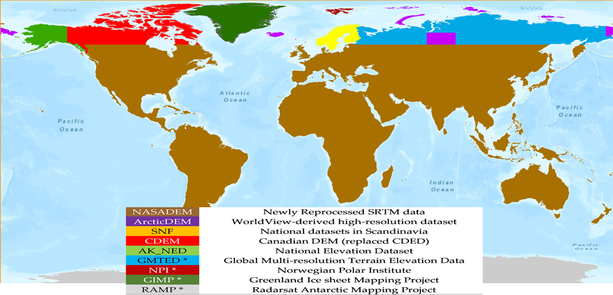
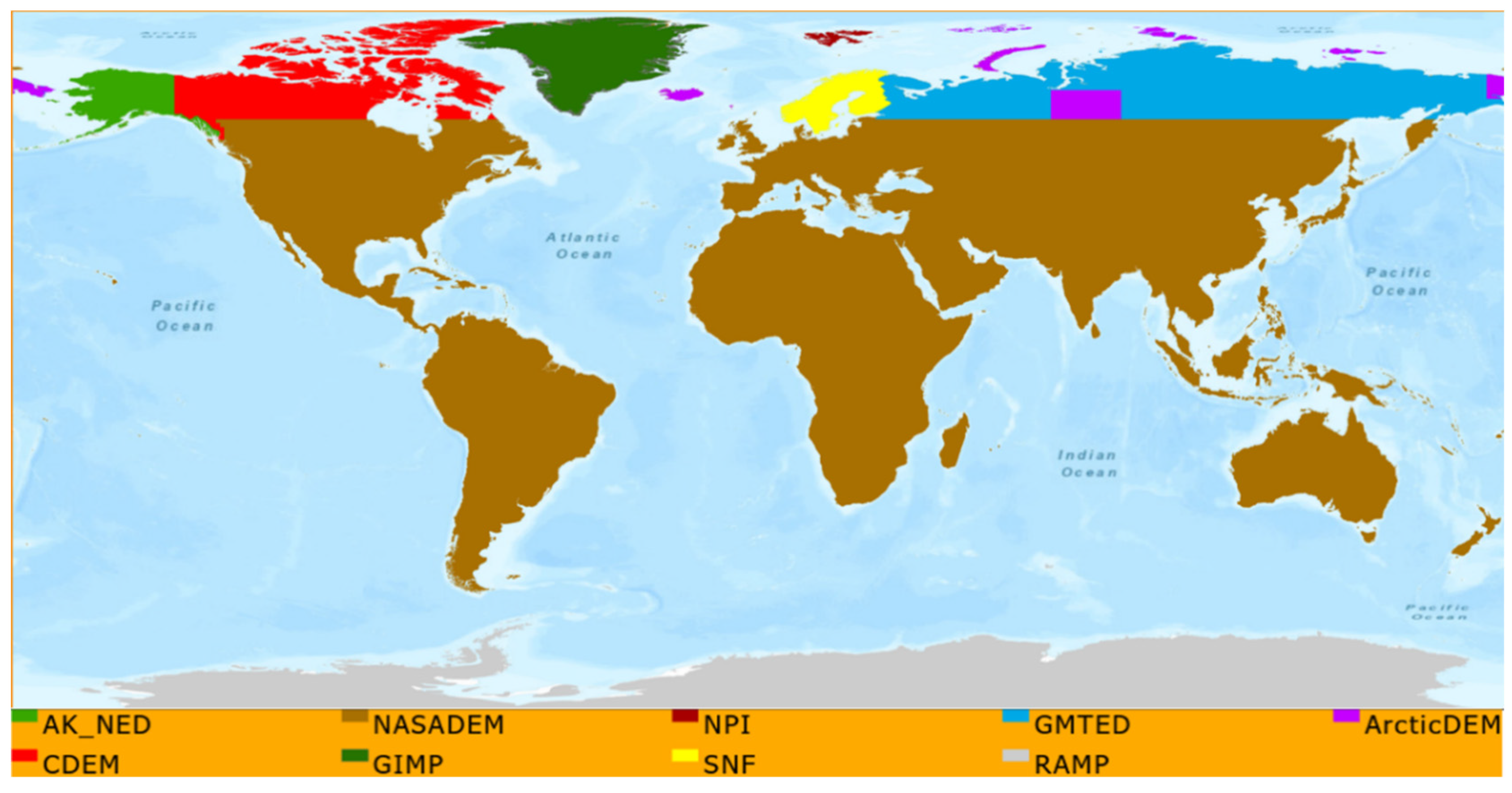
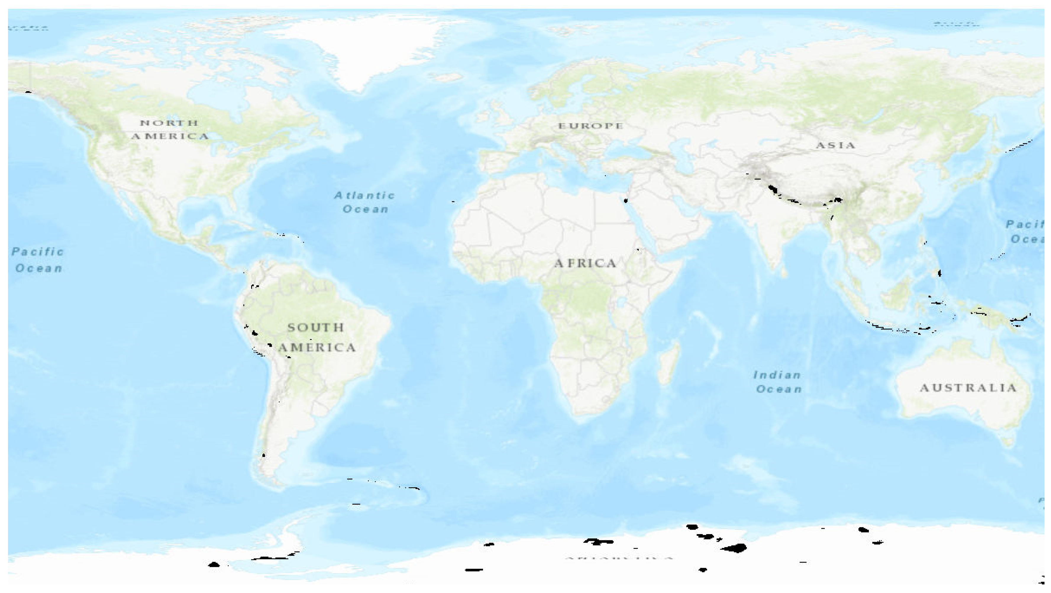
Various new DEM datasets were acquired and tested for their improvements over the current Collection-1 DEM. While several regions were not updated with a new DEM (denoted by an asterisk in

Table 1. Datasets that comprise new Landsat (Collection-2) Digital Elevation Model (DEM). The color of the headings shows where they are geographically in Figure 1.

	Full Name or Details	Region Used
NASADEM	Newly Reprocessed SRTM data	60°N–56°S
ArcticDEM	WorldView-derived high-resolution dataset	High Latitudes
SNF	National datasets in Scandinavia	Scandinavia
CDEM	Canadian DEM (replaced CDED)	Canada
AK_NED	National Elevation Dataset	Alaska
GMTED *	Global Multi-resolution Terrain Elevation Data	Russia
NPI *	Norwegian Polar Institute	Svalbard
GIMP *	Greenland Ice sheet Mapping Project	Greenland
RAMP *	Radarsat Antarctic Mapping Project	Antarctica

* These source datasets where not updated from Collection-1.

), most were. The datasets that comprise the new Landsat DEM and the regions where they will be used can be found in Table 1 and their geographical distribution can be seen in Figure 1.

2.1.1. NASADEM

The NASADEM dataset is a reprocessed DEM from the SRTM with many improvements to its quality and processing techniques. Additional elevation control from ICESat laser altimeter data (which did not exist during original SRTM production), in addition to improved radar interferometric unwrapping techniques, allowed for a more accurate product. Improved void filling was also applied by using concurrently produced GDEM3 [16], which allowed for synergistic improvements and greatly increased the quality of the NASADEM. NASADEM was created by the NASA MEaSUREs (Making Earth System Data Records for Use in Research Environments) program and was downloaded from the NASA LP DAAC (Land Processes Distributed Active Archive Center) [17]. The data are relative to the geoid (i.e., Orthometric) using the Earth Gravitational Model of 1996 (EGM96). Collection of the data is technically of the surface (i.e., Digital Surface Model), but the creators of the dataset (NASA Jet Propulsion Laboratory) claim that the radar does a good job penetrating the vegetation canopy so the Digital Terrain Model (DTM) bias is not large rendering the surface reference as a virtual DTM. The specific dataset that was used in the study was 1 arcsecondond, short integer void-filled data [2,18]. See

Table 2. Original specifications of evaluated DEMs.

Dataset	Pixel Size	Vertical Reference	Published Accuracy
NASADEM	1 arcsecond	EGM96 Geoid	4.0 m RMSE 1 [19]
ArcticDEM	5 m	WGS84 ellipsoid	Sub 1-m [20]
SNF	50 m	Geoid (version N/A)	N/A
CDEM	0.75 to 3 arcsecond	CGVD28 Geoid	see Figure 2
AK_NED	2 arcsecond	NGVD29 Geoid	2.44 m RMSE [21]
Collection-1 DEMs	3 arcsecond	EGM96 Geoid	varies per source

¹ Statistics are calculated only for North America.

for the original specifications of NASADEM and the other datasets evaluated in this study.

2.1.2. ArcticDEM

ArcticDEM data are produced by the Polar Geospatial Center (PGC) [22] using stereo high-resolution commercial imagery (mostly Worldview) for polar regions above 60 degrees north. Published absolute accuracy estimates are extremely high for this dataset, being sub-meter [20]. Since there are widespread voids [23,24], ArcticDEM data would have been difficult to use on a continental basis, so the decision was made to use ArcticDEM in localized regions and in northern island chains, where the Collection-1 DEM was known to have artifacts and inconsistent levels of accuracy due to multiple elevation sources used. Additionally, since Siberia is often clouded [25] and cloud coverage is one of the major factors in causing artifacts in optical data [26,27], there is an increase in the number of voids, in comparison to other northern regions where ArcticDEM has coverage. For this study, the 5-m mosaics were downloaded and used in the analysis. The dataset is vertically referenced to the World Geodetic System of 1984 (WGS84) ellipsoid and models the surface elevation (i.e., Digital Surface Model—DSM) [28].

2.1.3. Scandinavian DEM (SNF)

National datasets of Sweden, Norway and Finland (SNF) were produced by the Norwegian Mapping Authority, the Swedish Mapping Authority (Landmateriet) and the National Land Survey of Finland. These datasets were distributed at 25-m or 50-m pixel size and were projected to the Universal Transverse Mercator (UTM), zone 30 N coordinate system and mosaicked to create a single coverage. The dataset was vertically referenced to the geoid, so an elevation of zero is mean sea level (MSL).

2.1.4. The Canadian Digital Elevation Model (CDEM)

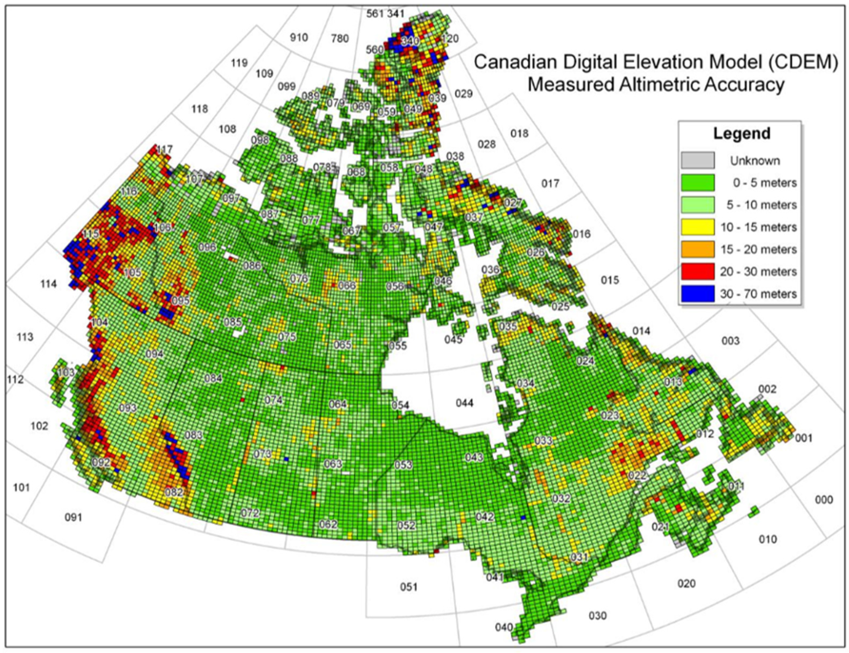
CDEM is produced by Natural Resources Canada (NRC) using an array of ground and reflective surface elevations. The post spacing varies per latitude from 0.75 to 3 arcseconds and the data are stored in geographic coordinates using the North American Datum of 1983 (NAD83) reference system. Vertical accuracy varies widely geographically, but in general is very good (see Figure 2). The dataset is vertically referenced to mean sea level using the Canadian Geodetic Vertical Datum of 1928 (CGVD28) geoid model [29].

2.1.5. National Elevation Dataset (NED)

The National Elevation Dataset (NED) is a seamless raster product primarily derived from USGS 10- and 30-m DEMs. NED data are available from The National Map Viewer [30] as 1 arcsecond (approximately 30 m) for all of the contiguous United States, and at 1/3 and 1/9 arcseconds (approximately 10 and 3 m, respectively) for parts of the United States. For Alaska, it is available as 2 arcsecond. NED data are distributed in a geographic projection and relative to mean sea level using the North American Vertical Datum of 1988 (NAVD88) geoid model for the United States and National Geodetic Vertical Datum (NGVD29) in Alaska.

2.1.6. Collection-1 DEMs Used in Collection-2

Four of the datasets used in Collection-2 were not updated from Collection-1. This was the case when there were no newer, superior data that were readily available. Those datasets were GMTED2010 in Russia, NPI in Svalbard, GIMP in Greenland and RAMP in Antarctica. Since these datasets were used in Collection-1, they have all been previously formatted to 3 arcsecondond resolution, projected to Lat/Long geographic and are relative to mean sea level using the EGM96 geoid. The original data specifications and characteristics are provided in the references: GMTED [31], NPI [26], GIMP [28] and RAMP [29].

2.2. Datasets Used for Comparison

2.2.1. Landsat Collection-1 DEM (GLSDEM)

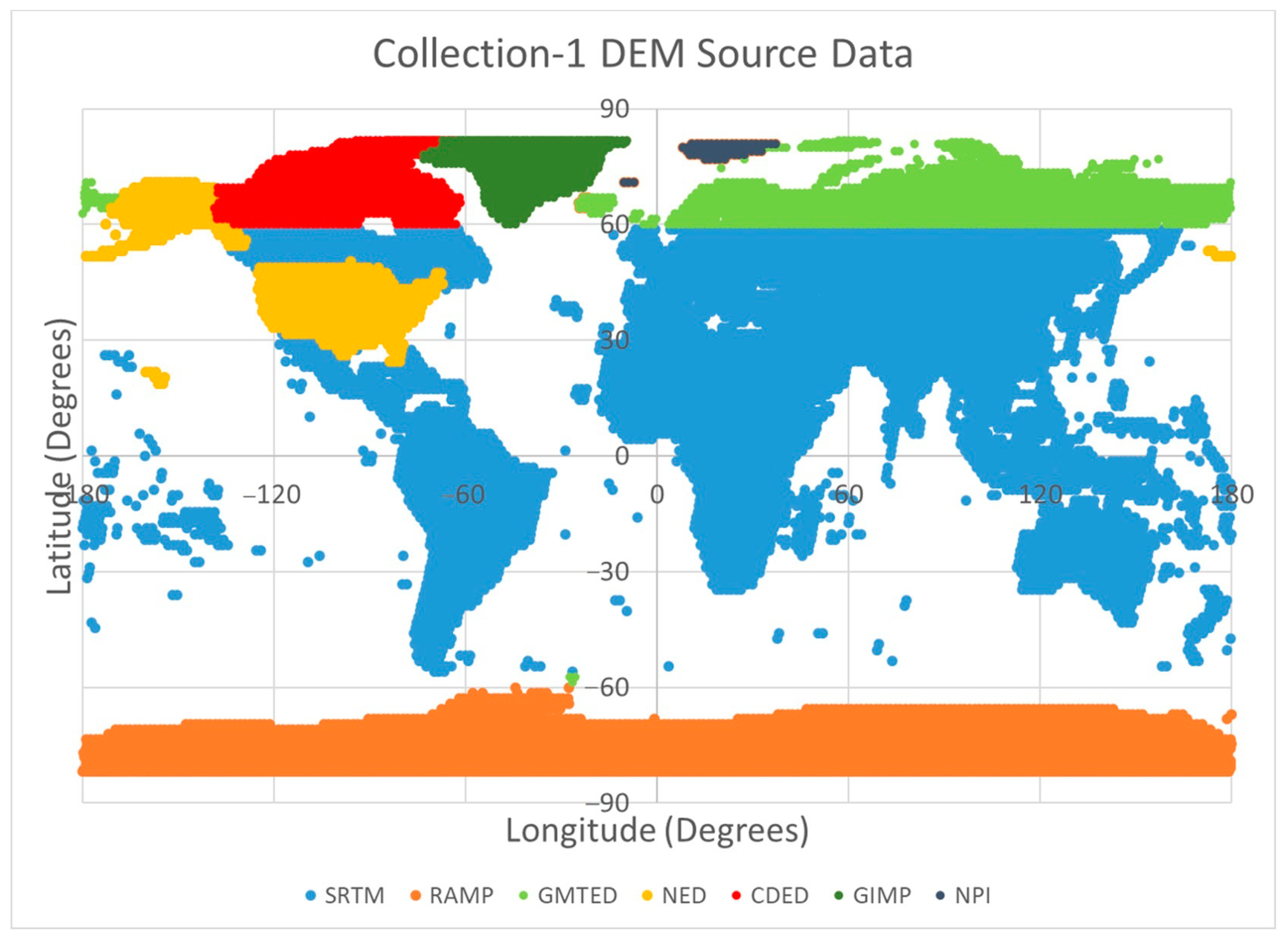
Since 2007, Landsat imagery has been orthorectified using virtually the same Digital Elevation Model because the Collection-1 DEM was not all that different from the original GLSDEM. Most of the elevation data for this dataset have come from the SRTM, which imaged the globe from 56°S to 60°N for 11 days consecutively in February of 2000 onboard the Space Shuttle Endeavor. While the overall absolute accuracy is roughly 10 m for most of the world, for latitudes north of 60 degrees, various other datasets were used in a “best available” approach (see Figure 3) with worst-case accuracies being 25 to 42 m root mean square error (RMSE) for GMTED [31] in the higher latitudes. This DEM was used to orthorectify the Global Land Survey 2000 (GLS2000), to which the entire Landsat archive was thereafter referenced [32]. The Collection-1 DEM will become a legacy dataset after the Landsat archive is reprocessed using Collection-2 sources.

These DEM renditions were also used to geometrically correct the popular image datasets GeoCover and GLS. These datasets were created for the epochs of the 1970s, circa 1990, circa 2000, circa 2005 and circa 2010 [32,33,34,35]. They were commonly used for studies of Land Use Land Cover Change (LULCC) before the complete Landsat archive was made publicly available at no cost in 2008 [36,37,38]. While these datasets mostly include the same elevation sources for orthorectification, the name was changed from GeoCover to the Global Land Survey (GLS) in 2007. That year, the GeoCover 2000 dataset was reprocessed to improve the geometric accuracy by using all available ground control points, Landsat-7 definitive ephemeris and tie points in a block configuration to create the GLS 2000 reference dataset [39]. Additionally, more widespread use of SRTM data was employed for the GLS, whereas for GeoCover it was only used in the continental United States and Alaska due to its provisional status [40]. After reprocessing using the improved geodetic information, the GeoCover datasets were renamed GLS [35].

From 2007 to 2020, the GLSDEM was used for all Landsat processing. This dataset has been stored in 1-degree tiles, 3 arcsecondond pixel spacing and referenced to mean sea level (MSL) using the EGM96 geoid. All the Landsat products in Collection-1 are corrected for terrain elevation effects using the GLSDEM, which is a mosaic of multiple sources of DEMs. Since the USGS is transitioning to a “Collection” version of this DEM, the “GLS” name will be replaced with “Collection-1”.

2.2.2. Esri-Served Airbus WorldDEM

The primary reference data used in this study to estimate error were from the Airbus WorldDEM elevation model served by the Environmental Systems Research Institute, Inc. (Esri) through their Geographic Information System (GIS) platforms. This DEM product is based on radar satellite data acquired during the TanDEM-X Mission, which is funded by the German Aerospace Centre (DLR) and Airbus Defense and Space. In regions of voids, the dataset was filled on a local basis with the following DEMs: Advanced Spaceborne Thermal Emission and Reflection Radiometer (ASTER), SRTM, SRTM90, SRTM30, SRTM30plus, GMTED2010, TerraSAR-X Radargrammetric DEM and the Advanced Land Observation Satellite (ALOS) World 3D 30-m. Published vertical accuracy is 2-m relative and 4-m absolute [41].

The Esri-served WorldDEM consists of the Airbus “WorldDEM4Ortho” data, an automatically generated elevation product created from WorldDEM DSM raw data, which is a hybrid between a DSM and DTM (Digital Surface/Terrain Model) [42,43]. This dataset is served at 0.8 arcsecond (approx. 24 m), and covers the entire Earth’s land surface, with pole-to-pole coverage. Access to this layer is provided as part of the Esri World Elevation Services dataset [44], through their “Terrain” layer and was parsed to only include the WorldDEM data source. Since these data are pulled from a server (as opposed to downloaded locally), changes can be made on the fly so there are many options to view and analyze. To most closely match the compared datasets, along with the base Collection-1 DEM, the format of the Esri WorldDEM data used in the study were referenced to mean sea level (i.e., Orthometric) using the Earth Gravitational Model of 2008 (EGM08) geoid.

Downloading the dataset is not possible; however, comparisons for testing purposes could be made using the Esri ArcGIS platforms. This dataset, with its global coverage, uniform collection methods and dependable accuracy, proved essential to this study for developing the accuracy statistics and for finding and analyzing artifacts.

2.2.3. Ice, Cloud, and Land Elevation Satellite (ICESat) Data

ICESat is the benchmark NASA Earth Observing System (EOS) mission for measuring ice sheet mass balance, cloud and aerosol heights, land topography and vegetation characteristics. From 2003 to 2009, the ICESat-1 mission provided multi-year elevation data for not only polar regions, but other areas including vegetation data around the globe. The ICESat-1 satellite was decommissioned in August 2010 [45]. The ICESat-1 time series product used in our analysis was GLAH14: GLAS/ICESat L2 Global Land Surface Altimetry Data. GLAH14 contains the land elevation and elevation distribution corrected for geodetic and atmospheric effects calculated from algorithms fine-tuned for over-land returns [46]. GLAH14 provides the surface height at a given point on the Earth’s surface at a given time relative to the WGS84 ellipsoid. To convert the elevation points to be relative to the geoid, the heights were converted using provided ancillary data.

The ICESat-2 satellite, which was launched in 2018 [46], has much better absolute accuracy [47], carrying the more advanced ATLAS sensor. However, due to its limited coverage at that time (our study started not long after the satellite was launched) we decided against using it. We were able to use the ICESat-1 sensor to some extent, but due to problems encountered with bad laser collects and because the sensors estimates heights of the Earth’s surface (i.e., DSM) and not the Earth’s terrain (i.e., DTM or DEM), we used it on a more limited basis than originally anticipated. Additionally, and while the effect is relatively small, both sensors onboard the ICESat-1 and ICESat-2 satellites suffer from unreliable height estimates with increasing slope and vegetation cover [47,48,49], which this study focused on. Lastly, these systems had limited ability to find surface imperfections and artifacts since it only samples the Earth with laser shots, rather than modeling the whole surface.

In an attempt to quantify how much impact the ICESat limitations would have on accuracy, we compared ArcticDEM, WorldDEM and ICESat-1 data over Iceland with one another to see if any of the datasets showed disagreement. The results indicated (

Table 3. Relative accuracy of ICESat-1 data over Iceland, compared to WorldDEM and ArcticDEM. No artifacts were removed (number of points = 96,381).

	Mean	STD	Range
WorldDEM—ICESat	−3.8	53.8	−2246 to 857
ArcticDEM—ICESat	−4.3	54.0	−2250 to 855
WorldDEM—ArcticDEM	0.6	6.3	−482 to 929

) that the difference between ArcticDEM and WorldDEM was less than that of the difference between ICESat-1 and WorldDEM or ICESat-1 and ArcticDEM. Therefore, we concluded that it was better to use WorldDEM as the reference than ICESat-1 since ICESat-1 did not agree well with either of the other two datasets. This poor agreement probably is due to the limitations we mentioned above. Nonetheless, ICESat-1 data were still useful as an independent evaluation of vertical accuracy, albeit not the primary source.

3. Methodology

To gauge improvement, the datasets were evaluated in two ways: (1) quantitatively, where the respective datasets were differenced from Esri-served Airbus WorldDEM data to ascertain how accurate the vertical estimations are; and (2) qualitatively, which looked for artifacts or data irregularities that would degrade the quality of the product orthorectification. In addition to the accuracy and quality assessments of the datasets, the potential for their inclusion was evaluated based on availability, consistency, and the difficulty of processing each dataset to the standards of the Collection-2 DEM. The Collection-1 DEM was also compared to the reference dataset and those results were compared to the results of the new DEMs to determine if the new datasets were an improvement over the Collection-1 DEM.

Since the Landsat Collection-2 DEM will have the same specifications as the Collection-1 DEM, all prospective datasets that were evaluated for their improvements first needed to be processed in various ways, depending on their original specifications (Table 2), to match that of the Collection-1 DEM. The Collection-1 DEM pixel size is 3 arcsecond, which is equal angle grid spacing in both longitude and latitude. All datasets evaluated for their improvement needed to be resampled to 3 arcsecond from their original pixel spacing and map projection. Some datasets needed cosmetic touch-ups, such as cleaning up inconsistent tile edges or converting water values to zero. Lastly, ArcticDEM data needed voids filled and the vertical datum converted to orthometric (see

Table 4. Dataset processing steps for each dataset to match Collection-1 DEM standards.

Dataset	Resampled 1	Reprojected to Lat/Long	Converted Water from Null to “0”	Cleaned up Water Edges 2	Filled Voids 3	Geoid Conversion 4
NASADEM	x
ArcticDEM	x	x		x	x	x
SNF	x	x	x
CDEM	x
AK_NED	x

¹ Resampling was done using cubic convolution. ² Edges were cleaned up using land water shapefiles. ³ Voids were filled following methods detailed in Section 3.2. ⁴ GDAL was used to convert to Orthometric units using the EGM08 geoid.

for the complete list of processing steps for each dataset). The only specification that was not always met was that the geoid model used for conversion did not always match. Since most datasets (all except ArcticDEM) were provided in orthometric standards, no conversion was needed. However, those datasets were not all referenced using the same geoid model as the Collection-1 GLS DEM, which was EGM96. CDEM used CGVD28, NED used NGVD29 and ArcticDEM was converted to orthometric using EGM08. Additionally, the two reference datasets that were used, WorldDEM and ICESat-1, were relative to the EGM08 geoid model [50]. Globally, the differences between EGM96 and EGM08 rarely exceed 5 m, mostly in Antarctica (see Figure 4). Nowhere do the differences exceed 11 m. As such, we did not expect this small difference in the reference geoid models to affect the analysis and the results shown in this study. For example, in the high latitude regions where ArcticDEM was used, the differences between EGM96 and EGM08 geoids is less than 3.5 m. In contrast, the differences between the Collection-1 and Collection-2 dataset sources were greater than 35 m. The differences between the EGM08 geoid and CGVD28 or NGVD29 are likewise small, being less than 2.5 m in Canada and the United States, where they were used [51]. The main features of the reference data used in the analysis can be found in

Table 5. The main features of the reference data.

Reference DEM	Pixel Size	Projection	Statistical Comparison	Surface Reference	Geoid
Esri WorldDEM	3 arcsecond	Geographic	Raster differencing	DSM/DTM	EGM08
ICESat-1 GLAS	70 m	UTM	Point differencing	DSM	EGM08

.

3.1. Methods Used to Access, Prepare, and Use Reference Datasets

3.1.1. Airbus WorldDEM Data

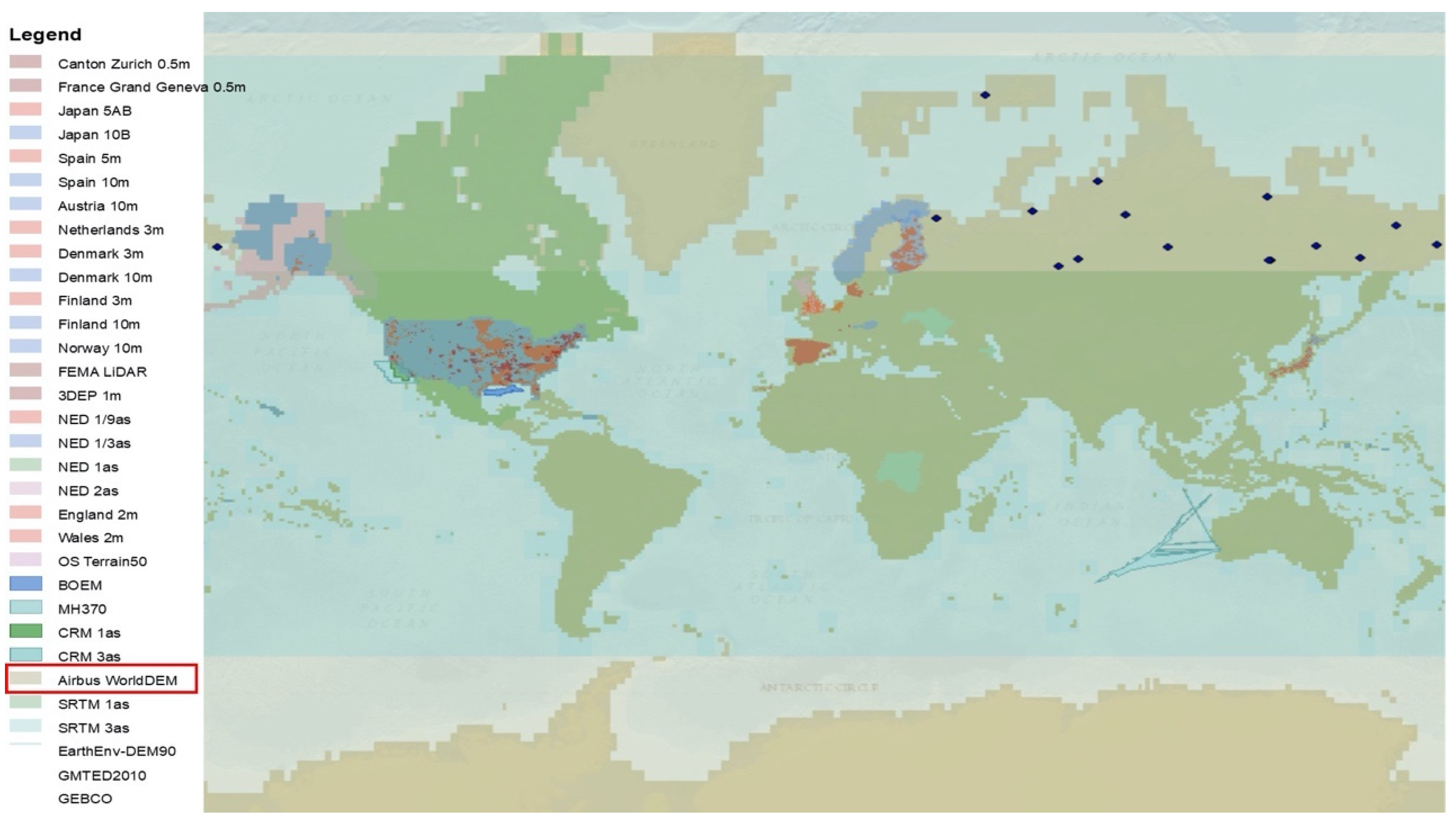
The Esri-served WorldDEM data are available through Esri World Elevation Services for use within the ArcGIS Online platform and are part of the Living Atlas. The entire collection of layers can be accessed from within the Elevation Layers Group on ArcGIS online. Access to these global layers is free, but an ArcGIS organizational account is needed. Once within the Elevation Layers group, the “Terrain” layer was accessed, which is a dynamic collection of elevation datasets. These datasets are based on multiple sources at multiple resolutions (See Figure 5 for a subset of the sources). The mosaic was stacked with all available elevation layers, such that higher resolution datasets were displayed at higher priority. To “lock” the layers to only evaluate Airbus WorldDEM, a definition query was set to only use data from that source. This was done to assure that when differencing the datasets, it was against the WorldDEM data and not from one of the other layers in the dataset.

Once the WorldDEM layer was isolated for analysis in ArcGIS, it was differenced from the various datasets of interest, giving statistics of the mean, standard deviation and the range of the differences between the DEM of interest and the WorldDEM. The statistics from the differenced datasets were used to determine the relative accuracy, since the Airbus WorldDEM was being used as the main reference. For those same regions for each new DEM, the Collection-1 DEM was also differenced from WorldDEM and those statistics were compared against the ones derived from differencing the new DEMs. It was those comparative statistics that determined which DEM (the new DEMs or the Collection-1 DEM) was more accurate.

3.1.2. ICESat-1 Data

Preparing the ICESat data where they could be used in our analysis had many steps. The data were first downloaded as ACSCII files from NASA’s Earthdata website [52]. To eliminate problematic returns, the data points were filtered for cloud-contamination, saturation and fill values (from the quality flags). To match the vertical reference frame of the Collection-1 DEM, ellipsoidal heights were converted to orthometric by applying the geoid separation value (found in “d_gtHt” file) for each point using the accompanying ancillary data (found in the “Geophysical” folder).

Even after the filtering, there still were points with erroneous values, mostly close to filtered-out clouds, high vegetation, or regions with steep topography. Those points were further screened by comparing them to the Airbus WorldDEM and removed if the ICESat data points were inconsistent with WorldDEM by more than 50 m (i.e., differences >50 m are probable errors in the ICESat data).

Northeast Russia is an example where ICESat data were used, and where it was suspected that the Collection-1 DEM was unreliable due to the presence of apparent artifacts such as large tile-to-tile discontinuities. In this area we wanted to test for improvement using ArcticDEM, but we also knew that processing the ArcticDEM would be difficult since it had many voids in that region. Instead of solely trusting WorldDEM data in that area, we wanted confirmation that by switching to ArcticDEM it would be a significant improvement, so we used ICESat data for this confirmation. The Collection-1 DEM was first differenced from WorldDEM and then was compared to the difference between void-filled ArcticDEM and WorldDEM. Noting that this showed a significant improvement, we then confirmed that result by making the same comparison using the ICESat-1 layer (see Figure 6 and

Table 6. Comparative results using WorldDEM and ICESat-1 as reference datasets in northeast Russia.

	Mean		STD		Range
Reference Dataset	Collection-2 1	Collection-1	Collection-2 1	Collection-1	Collection-2 1	Collection-1
Airbus WorldDEM	1.0	2.7	8.5	37.0	−467 to 456	−634 to 450
ICESat-1 data	0.7	−2.0	3.7	19.7	−36 to 35	−887 to 210

¹ In this region, the Collection-2 data source are ArcticDEM.

). Note that the reason the ICESat-1 data in Table 6 shows more agreement with ArcticDEM, while in Table 3 they show much less agreement is that the ICESat points that were used in Table 6 had the secondary filtering done, where the additional bad (i.e., >50 m from WorldDEM) returns were eliminated.

3.2. ArcticDEM Void Filling

Void filling of the ArcticDEM data were necessary to have a complete dataset without holes where data are missing. The smaller voids were interpolated over using a plane fitting/inverse distance weighted (IDW) interpolation method offered by Esri software specifically designed for filling DEM voids [53]. For larger voids, where the interpolation method could not successfully cover, we employed a fill method that used ASTER GDEM (Global Digital Elevation Model) and the original Collection-1 DEM. The procedure used was to bias the hole filling dataset (e.g., GDEM) to match the ArcticDEM data using common points around the perimeter of the void area, insert the biased fill data to replace the void areas and then smooth the patched area to suppress discontinuities at the seams. In addition to treating voids in this manner, this process was also used for WorldDEM identified artifacts (regions where differences were greater than 50 m) in the ArcticDEM data. Those identified regions were extracted and then refilled using the same interpolation/filling method. An example of the process is shown in Figure 7 of the Zemlya Gorga Islands off the northern coast of Russia. First the ArcticDEM layer was differenced from WorldDEM to obtain initial statistics, then the voids and large errors were identified and fixed and lastly the difference statistics were re-calculated. In this example, there were no holes in the ArcticDEM data that were not able to be fixed by interpolation, so filling was not necessary. The improvement in the difference statistics (

Table 7. Difference statistics, in meters, between ArcticDEM and WorldDEM before and after filling voids in ArcticDEM data of Zemlya Gorga Islands.

	Mean	STD	Range
Initial difference	0.95	6.3	−886 to 224
Final difference	0.96	5.9	−128 to 126

) were not large, but the objective was mostly to fill the voids, not to improve the statistics.

3.3. Artifact Detection

Since most of the Collection-1 DEM consisted of SRTM data, which are known to have artifacts, it was necessary to develop an algorithm to search for the artifacts rather than visually review the images. This was accomplished by using a topographic modeling tool [54] in ENVI^® software to calculate slopes within the DEMs, based on the premise that irregularly high slopes found in an image are probably attributed to an artifact of some sort, like a pit, spike, or void. This tool was scripted in IDL to calculate the slope values (Equation (1)) found for each pixel in each image and create a flag if that value was greater than a threshold:

$$slope \left(percent\right)=100\ast \sqrt{{\left(\frac{dz}{dx}\right)}^2+{\left(\frac{dz}{dy}\right)}^2},$$

(1)

where d_z is the change in elevation over a given distance in longitude, d_x and latitude, d_y.

For the SRTM tiles that were flagged, the same script was run on the corresponding NASADEM tiles to learn if similar slope values were present, with the assumption being that if the high slope values were only present in the Collection-1 DEM, then an artifact is the most likely cause. Additional statistics for the flagged tiles were printed, giving information about the normal distribution of values and helping to determine what other slopes were found in the tile. Because of the high degree of variability around the globe, the slope thresholds varied depending upon the region of interest and other slope values found in the region, but they varied from 350% to 600% (74° to 80° angle). 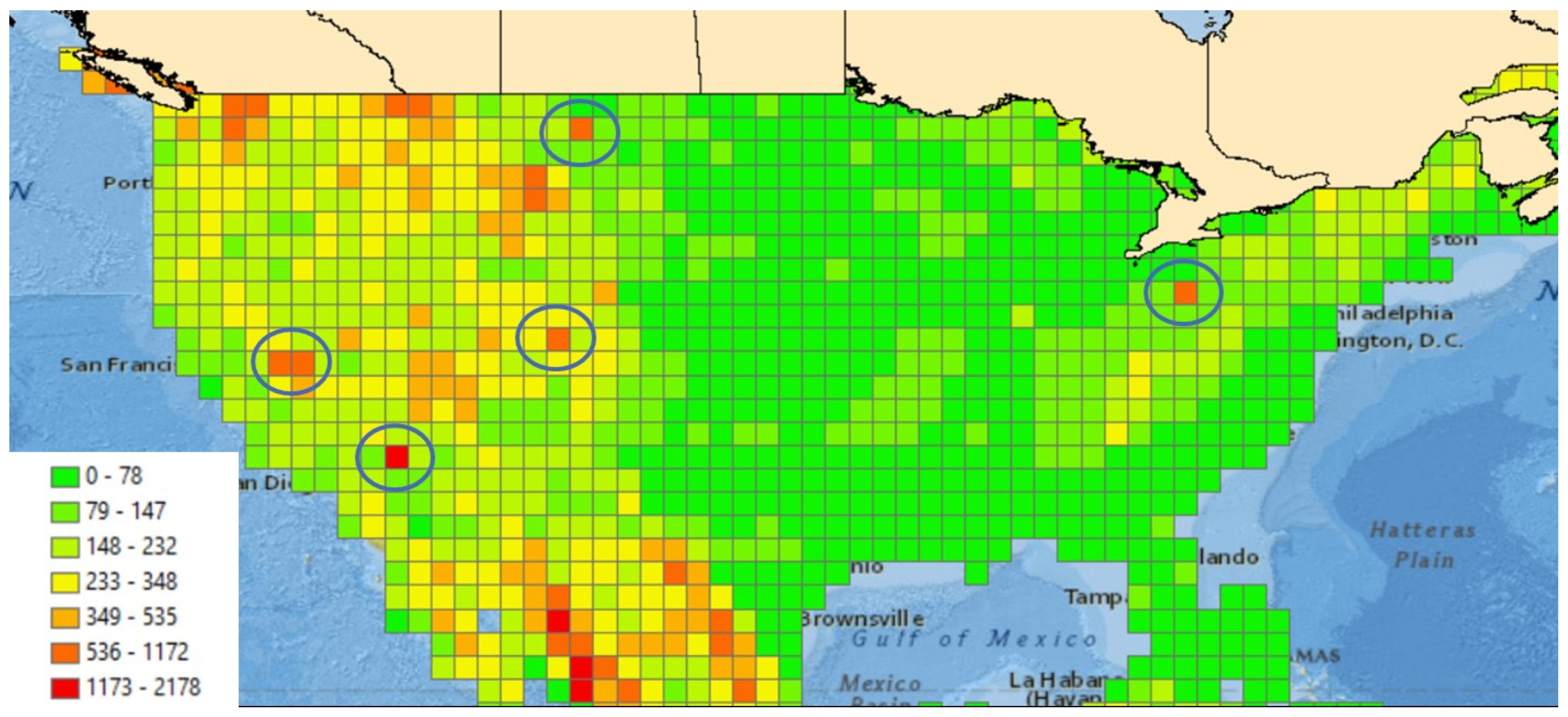A flow diagram of the artifact detection algorithm can be found in Figure 8. Furthermore, mapping the maximum slope values found in each tile helped to isolate unusual values, as surrounding tiles in the same geographic region should typically have similar steepness. Figure 9 shows an example in the United States where several tiles exhibit outlier behavior when compared to the slope values of its neighbors. Between flagging high values of slopes within the imagery, comparing those slopes to the normal distribution of values and mapping the maximum slopes of its neighboring tiles, we were able to identify tiles that were suspect and should be further inspected for artifacts.

4. Results and Discussion

The goal of this study was to evaluate newly available digital elevation datasets for their improvement over the current Collection-1 DEM and their potential for inclusion into a newer Collection-2 DEM that is currently under development.

4.1. Qualitative Assessment

As the various elevation datasets were being evaluated, special attention was paid to irregularities that would hinder or otherwise degrade the value of each source when compiling the global dataset that will be used for Landsat orthorectification. Artifacts play an important role in the orthorectification process because large irregular errors in the elevations develop into large horizontal geodetic errors, locating pixels in the wrong places and causing visual image discontinuities. Note that artifacts were discovered in different ways since no single method proved successful in detecting all DEM flaws. For example, the slope detection algorithm proved effective for finding the pits, spikes and voids, but it did not work well for artifacts that did not cause sharp slopes as in the case of washouts. Those types of artifacts predominately appeared in mountainous regions and were found easily by visual assessment. Additionally, other artifacts such as the tiling pattern that was discovered in Scandinavia was only discovered by differencing two layers. In summary, some artifacts were found by searching for them using a developed method, like that of the slope detection algorithm, while others were discovered in a less formal fashion either when visually looking at the DEM or when differencing layers and noticing odd patterns. Below are some of the more striking examples that were found.

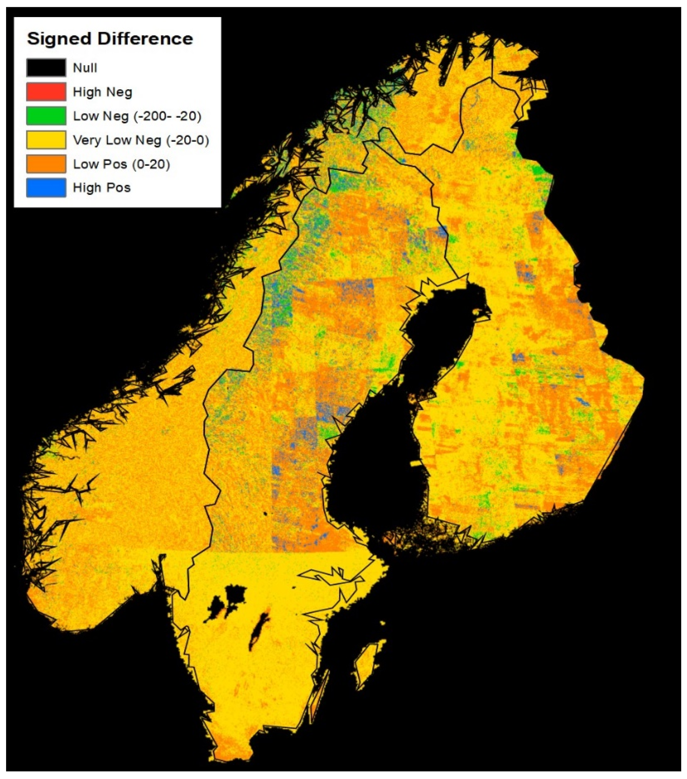
When differencing the Scandinavian (SNF) dataset against the Collection-1 DEM, a significant tiling pattern was distinguished in Sweden (Figure 10). To determine if the tile pattern was due to irregularities in the SNF dataset or the Collection-1 dataset, looking at the datasets individually and zooming into the most dramatic areas revealed that the tiling pattern lay within the Collection-1 DEM. Looking at the differenced layer (Figure 10) of the datasets also highlighted where the source data for the Collection-1 DEM dataset changed. Above 60° north latitude, not only was there the tiling artifact, but substantially more variability between the datasets was found. The variability is because above 60° north the source data for the Collection-1 DEM is GMTED, whereas below 60° north it is SRTM, which shows much more uniformity and consistency. In summary, although this tiling pattern was found when analyzing the SNF dataset, the pattern was due to the irregularities in the Collection-1 DEM source data (GMTED) for this region. As such, this substantiated that a switch to the SNF DEM for Scandinavia was warranted.

ArcticDEM data were one of the most anticipated new datasets being considered for inclusion in the Collection-2 DEM. Not only does this dataset have extremely high accuracy, on par with WorldDEM when resampled to 3 arcsecond, but above 60° north latitude is the zone where the Collection-1 DEM is most challenged due to the use of many different datasets with varying levels of quality and source resolutions. ArcticDEM was completed and updated in phases (called “releases” by PGC) as more regions were processed and more voids were filled. Their final release (release 7) was the version that was evaluated in this study and used in the generation of the Collection-2 DEM. While many of the voids were filled in comparison to earlier versions of the dataset, there remained a substantial amount of void area, which made ArcticDEM unsuitable for wholesale replacement. 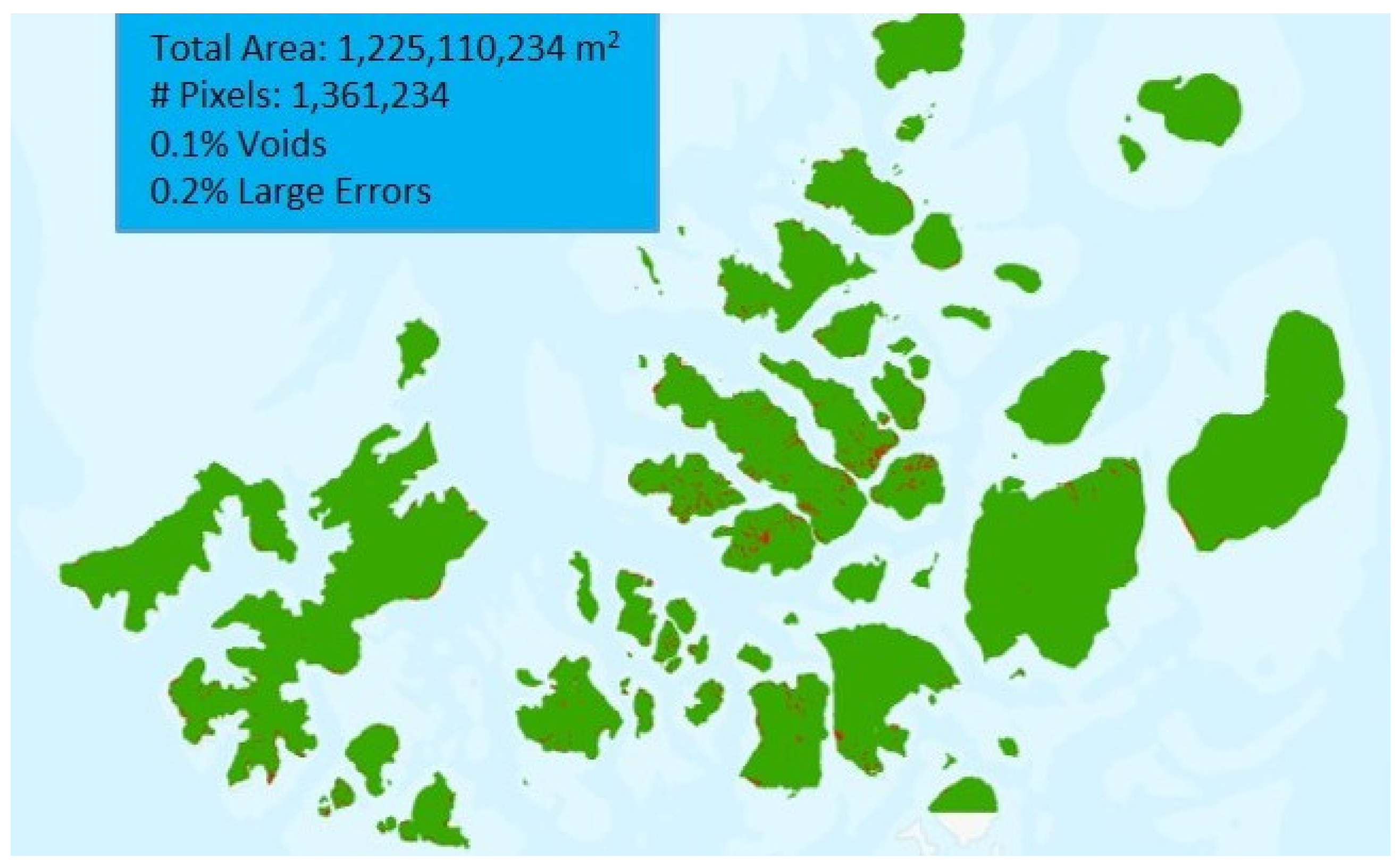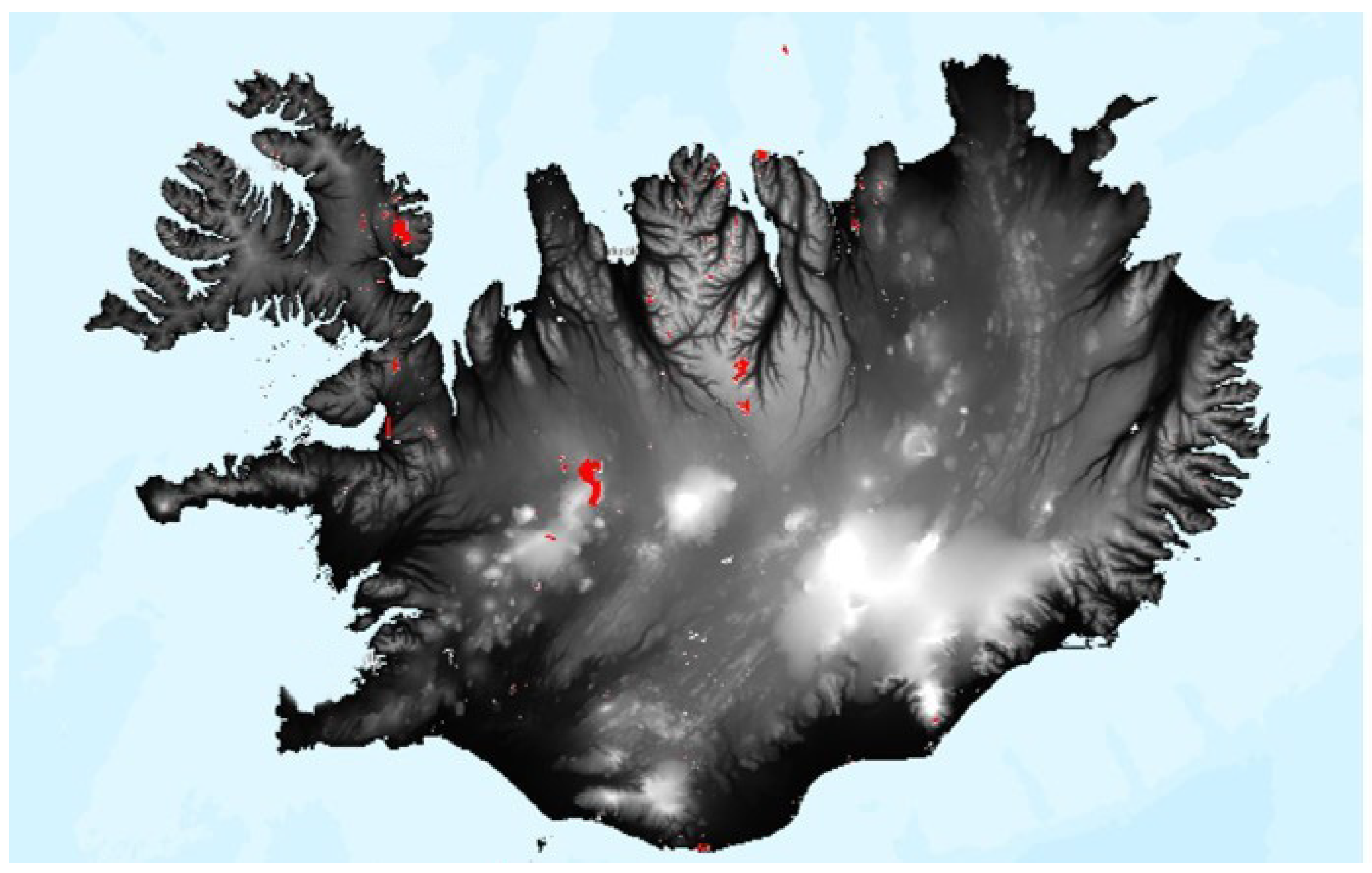Figure 11 shows an example of where ArcticDEM was used over Iceland and the voids are still present in release 7. Without zooming closely into the DEM image only a handful of the voids in the figure can be visually observed, but the voids were numerous. In the Iceland example, the number of voids that needed to be filled was 863. While a method was developed to compensate for the voids, the labor involved in this process limited the usability to smaller regions where newer data were most needed. The hope is that in the near future, producers of the ArcticDEM dataset will be able to ensure that their dataset is void free for all regions north of 60 degrees where SRTM is unavailable. Doing so will certainly benefit the scientific community as there are not many freely accessible datasets available in these regions that are as accurate as the ArcticDEM.

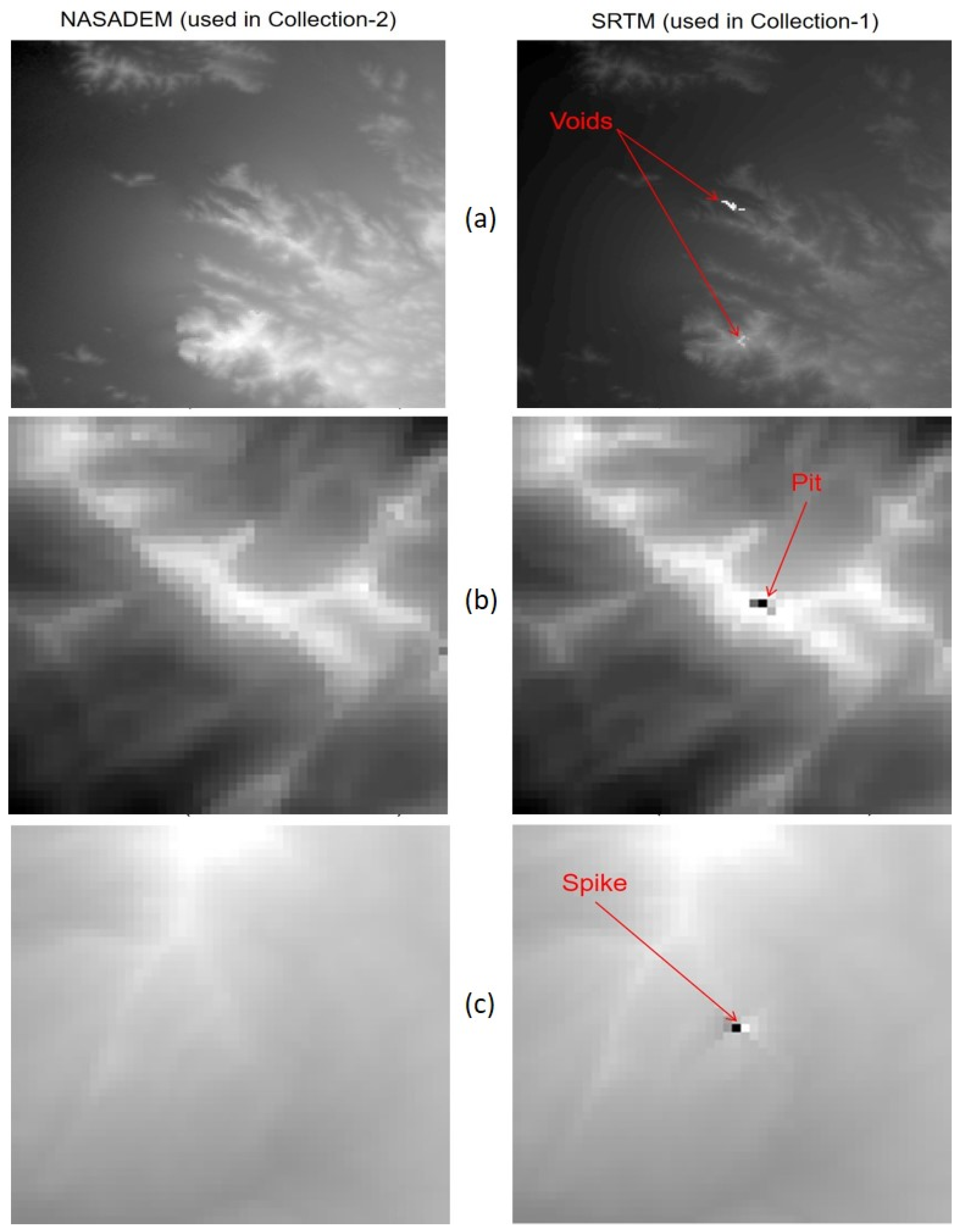
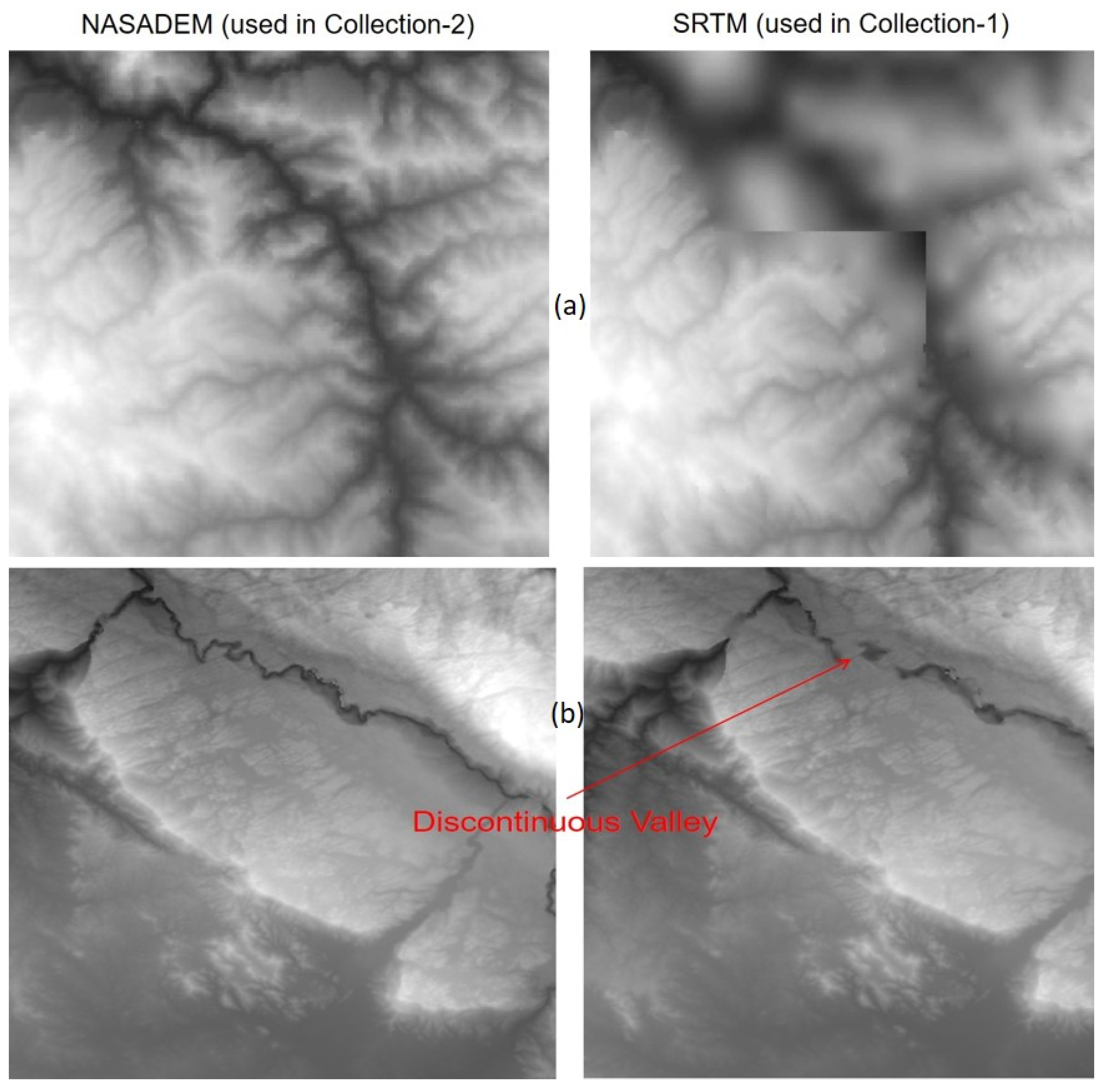
The Collection-1 DEM uses SRTM data as its primary elevation source for most of the globe, covering everything from 56° south to 60° north latitude. With such a vast landscape, finding artifacts in the SRTM imagery benefited by using an artifact detection algorithm that calculated slopes to highlight tiles with potential problems. Numerous artifacts in the SRTM imagery were highlighted and corrected in NASADEM reprocessing, including voids (Figure 12a), pits (Figure 12b), and spikes (Figure 12c), all of which were found using the artifact detection algorithm. Other types of artifacts that were found by other means where washouts (Figure 13a) and other minor artifacts (Figure 13b). In total, 21 tiles containing artifacts were found in the SRTM data using the artifact detection algorithm (

Table 8. Artifacts found in SRTM data using slope analysis algorithm, per region.

	Number of Tiles Analyzed	Artifacts
United States	1169	7
MX/C.A./Caribbean	447	2
South America	1738	1
Africa	2755	1
Europe	1333	1
NE Asia	4066	4
SE Asia	709	5
South Pacific	920	0
	13,137	21

). Many of the artifacts were found in high elevations of Asia where there is a more widespread benefit to using NASADEM due to its higher fidelity in regions with steep slopes. The least number of artifacts were found in regions of lower elevations, including the South Pacific, where no such artifacts were found. The increased quality of NASADEM, especially in the mountainous regions, was the largest reason why it was accepted into the new Collection-2 DEM, as no evidence of an overall improvement in accuracy was found.

4.2. Statistical Assessment of Datasets

To estimate a measure of accuracy in the compared datasets, the Esri-served WorldDEM was used as a reference to which the prospective DEMs were compared by differencing the layers. This WorldDEM dataset covers the entire globe and the collection strategy was uniform throughout. This was important, as it would have been difficult to compare the accuracy of various datasets if the reference for each dataset was different or if the quality was not uniform. As noted previously, our goal was not to ascertain absolute accuracy, but rather to get a measure of consistency between compared DEMs to make a judgement as to which ones are best to include in the new Collection-2 DEM.

All the evaluated DEMs were compared to the Esri-served WorldDEM layer and statistics of those differences were used to gauge accuracy. The statistics for those comparisons are provided in

Table 9. Dataset comparisons against WorldDEM, in meters. Colored headings are to help in locating datasets, geographically, in Figure 1.

	Mean		Standard Deviation
	Collection-1	Collection-2	Collection-1	Collection-2
NASADEM	0.8	1.1	26.8	11.2
ArcticDEM	0.9	−0.1	42.2	6.8
SNF	0.1	1.6	13.8	6.7
CDEM	1.6	−1.6	31.1	12.4
AK_NED	−2.6	−1.0	28.1	10.2
GLS DEM *	−1.8		18.2
NPI *	−3.5	1.6	20.7
GIMP *	−2.8		24.3
RAMP *	−0.2		58.7

* These source datasets were not updated (i.e., the values would be the same in Collection-1 and Collection-2 DEM).

.

ArcticDEM was used in the Arctic Islands and a few problem areas in Northeast Asia. These regions replaced with ArcticDEM had the greatest improvement, with differences from the reference layer having a standard deviation of 42.2 m in the Collection-1 DEM, whereas for the Collection-2 DEM, the standard deviation was 6.8 m, showing much better agreement. This was important as these regions had known quality issues. ArcticDEM was an excellent substitute and would have been much more widely used for all of Siberia if not for the numerous voids currently contained in the dataset.

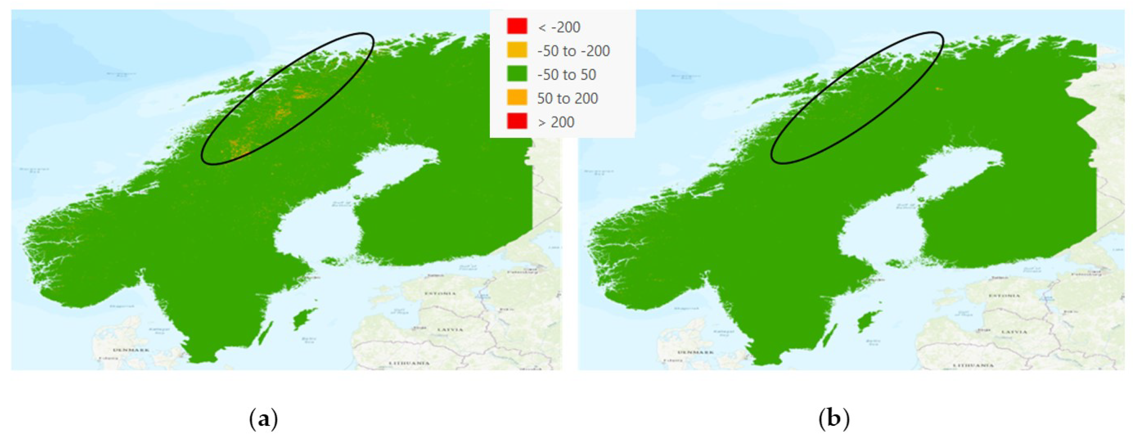
The accuracy of the Scandinavian dataset (SNF) was about twice that of the Collection-1 DEM, with the standard deviation between the SNF and reference dataset decreasing from 13.8 to 6.7 m. This resulted in accuracy close to that of ArcticDEM, with both being slightly less than 7 m from the reference layer. Most of that improvement was along the Scandinavian Mountains on the Norway/Sweden border as can be seen in Figure 14. Using the SNF dataset also cleaned up the blocking pattern that was observed above 60° north in the Collection-1 DEM (Figure 10).

Upgrading to CDEM was strongly indicated since the previous CDED dataset was no longer supported by Natural Resources Canada (NRC) [10]. Indeed, the accuracy of the height estimates in Canada improved considerably when compared to the reference dataset (see Table 9). The Canadian NRC has an even newer dataset that they created, called High Resolution Digital Elevation Model (HRDEM), which is a combination of ArcticDEM and Light Detection and Ranging (LiDAR) sources. Both HRDEM and ArcticDEM are more accurate than CDEM, but HRDEM was not complete at the time of this study and ArcticDEM was not used because of numerous voids (even in their final release 7 version).

For both the NED dataset in Alaska and everywhere below 60 degrees north where NASADEM was evaluated, the results were similar. There were no large differences in the flat regions, but in mountainous regions, there tended to be more artifacts in the Collection-1 data, and this is where the newer datasets greatly improved the Collection-2 DEM. The correction of the artifacts is what drove the improvements of the statistics when compared to the reference layer. Similar trends appeared in both the NED and NASADEM areas, with the vertical error reduced by 16 to 18 m compared to the Collection-1 DEM, mostly due to the aforementioned correction of artifacts. This was a significant amount of improvement and shows how much the correction of artifacts can improve the accuracy of a DEM.

Regarding the other data sources that composed the rest of the Collection-1 DEM, we decided not to make an update and those sources were carried over to be used in the Collection-2 dataset. For these regions, covering Svalbard, Greenland, and Northern Siberia, we retained the Collection-1 DEM tiles as their relative accuracies are in line with the other improved datasets. Additionally, they have relatively flat terrain and therefore are less likely to introduce horizontal errors in the Landsat orthorectification process.

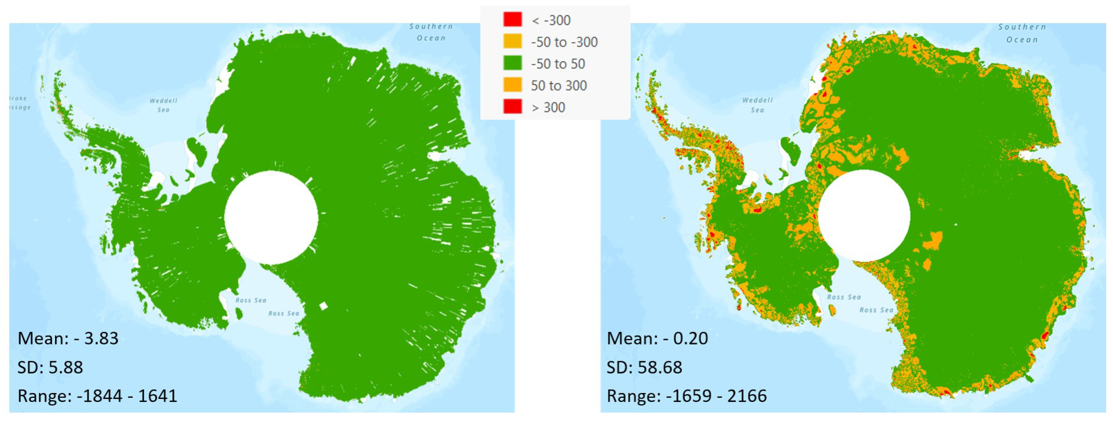
The RAMP dataset over Antarctica was retained for a different reason. It was clear from the statistics that this dataset leaves much room for improvement in terms of accuracy, having a difference in the standard deviation from WorldDEM close to 60 m. We considered using the Reference Elevation Model of Antarctica (REMA) DEM to replace RAMP, as this dataset had much more agreement with WorldDEM (see Figure 15). Clearly the REMA dataset is better accurate than RAMP, but it is incomplete and has too many voids to consider, since it uses the same methodology that is used to generate ArcticDEM. Release 2 for REMA is not yet completed but is supposed to fill many of the voids.

4.3. Geometric Accuracy Improvements

Improvements in the absolute precision of the Digital Elevation Models (DEMs) used for scene orthorectification will affect final Landsat Level-1 Precision and Terrain (L1TP) geolocation in different ways. This is a function of both the topography of the individual scene and the accuracy improvements of the DEM.

Table 10. Horizontal Geodetic Improvement, in meters.

	Mean	STD	Min	Max
NASADEM	0.0	0.4	−367.0	360.0
ArcticDEM	0.0	1.5	−104.0	88.0
SNF	0.0	0.8	−84.0	70.0
CDEM	0.0	1.6	−156.0	156.0
AK_NED	0.0	1.7	−189.0	179.0

shows the estimated improvements, in meters, in location accuracy the improved DEMs will provide. The differences in some datasets will lead to geolocation improvements of up to hundreds of meters. The script used to calculate these values considers the differences in elevation estimates along with the viewing geometry of the Landsat sensor in the Worldwide Reference System-2 (WRS-2) grid to compute parallax. Off-nadir observations with large DEM differences produce the largest horizontal displacements. This calculation was used to learn which areas to expect the largest differences in horizontal error based on improved vertical accuracy of the DEMs.

The largest improvement in geodetic accuracy is in the region where original SRTM data from Collection-1 will be replaced with NASADEM data in Collection-2. Interestingly, however, this is not the dataset that is improving the most in vertical accuracy (see Table 9); that title belongs to ArcticDEM. This improvement is due to a combination of factors. First and foremost, it is primarily driven by artifacts in the DEM and not necessarily due to large systematic error. Additionally, the topography of the regions where ArcticDEM was used is not as mountainous as in parts of Asia where NASADEM will be used and, consequently, where the largest geodetic improvements are found. The WRS path and row that showed the greatest improvement due to the more accurate DEM was Path 150 Row 35, in the Himalayan Mountains of Pakistan. In this most affected area, the horizonal accuracy will be improved up to 12 pixels (360 m) for the regions where a dramatic artifact is coupled with off-nadir viewing geometry. It is important to note that the whole image is not shifted or misplaced at this magnitude, but only the area within the image around that specific artifact. Satellite sensors, like those found on Landsat, only view off nadir up to 7.5 degrees at its edges. Other sensors, especially those that can point at greater off-nadir angles will be even more affected by DEM inaccuracies as parallax increases at those geometries.

5. Conclusions

In 2017, the USGS initiated a study to determine if better DEM datasets were available than were currently being used to orthorectify Landsat data. The Collection-1 DEM has sources that were collected up to 20 years ago, and the improved geometric accuracy of newer data will improve the accuracy of the horizontal placement of Landsat data in the orthorectification process. The improved global elevation dataset from this study, referred to in this document as the Landsat Collection-2 DEM or simply Collection-2 DEM, will be used to process all past, present, and future Landsat images and is expected to be released by the end of 2020.

The new global DEM update is complete. Elevation sources used for the updated dataset include NASADEM (where SRTM was previously used in Collection-1), CDEM (Canada), NED (Alaska), national datasets (Scandinavia, Svalbard, Jan Mayen), GIMP (Greenland) and ArcticDEM (Iceland, Faroe Islands and selected high latitude areas). The most important benefit of the new Collection-2 DEM when compared to the Collection-1 DEM is the reduction of artifacts, as large absolute errors introduced by artifacts have the largest impact in terrain correction of satellite imagery. Many voids, spikes, pits and other inconsistencies found in the Collection-1 DEM have been identified and fixed in the Collection-2 DEM. All dataset updates improved the vertical accuracies by more than a factor of two in comparison to the Collection-1 DEM dataset, with the biggest improvement in regions where ArcticDEM was used with vertical accuracy improving from over 42 m to under 7 m, when compared to the Airbus WorldDEM reference layer. The effect of improved vertical accuracy in the DEM for Landsat orthorectified products showed an improvement of over 300 m in horizontal displacement for a DEM artifact with worst-case Landsat view geometry. This large horizontal error is primarily driven by the localized artifacts in the DEM tiles (spikes/pits) and is not to be confused with the horizontal mis-registration error for the entire scene. The parts of the globe where the Landsat DEM was not updated were in northern Siberia (mainland), Svalbard, Greenland and Antarctica. The DEM in those regions will most likely be updated in Landsat Collection-3.

Airbus WorldDEM (via Esri) and ICESat-1 data were used as validation data sources. While ICESat-1 data could have been useful for assessing overall dataset accuracy if additional filtering was applied, it was not used as the primary source to gauge accuracy. This was because ICESat was found to exhibit artifacts near regions identified as clouds when using the normal quality flag information. Additionally, ICESat are point data and were not found suitable for modeling the complete surface to find anomalies such as artifacts, which was a major factor for quality assessment. In the future, validation using ICESat-2 and Global Ecosystems Dynamics Investigation (GEDI) data would be best as they have better accuracy than either ICESat-1 or WorldDEM. However, WorldDEM was more than sufficient for the needs of this study and using more accurate reference data most likely would not have changed the results. Additionally, a raster layer would still be necessary as both ICESat-2 and GEDI are sampling sensors that would not model the complete surface, and hence not find all artifacts. WorldDEM’s properties make it suitable for assessing both accuracy and the presence of artifacts.

It should also be mentioned that in some cases, having a newer Landsat DEM may cause other problems, even if it is more accurate. There are instances, such as when landslides or volcanic eruptions occur, where the actual topography has changed and by introducing a new DEM and applying it to older data, it may misregister the land. This will be a limitation to the “collections” strategy that the USGS is following and users should be careful in localized regions where such dramatic land transformations have occurred.