Article

Sentinel-1 and Sentinel-2 Data for Savannah Land Cover Mapping: Optimising the Combination of Sensors and Seasons

1
Department of Natural Sciences, Manchester Metropolitan University, Manchester M15 6BH, UK
2
School of Mechanical, Aerospace and Civil Engineering, University of Manchester, Manchester M13 9PL, UK
*
Author to whom correspondence should be addressed.
Remote Sens. 2020, 12(23), 3862; https://doi.org/10.3390/rs12233862
Submission received: 5 November 2020 / Revised: 18 November 2020 / Accepted: 23 November 2020 / Published: 25 November 2020

Abstract

:
Savannahs are heterogeneous environments with an important role in supporting biodiversity and providing essential ecosystem services. Due to extensive land use/cover changes and subsequent land degradation, the provision of ecosystems services from savannahs has increasingly declined over recent years. Mapping the extent and the composition of savannah environments is challenging but essential in order to improve monitoring capabilities, prevent biodiversity loss and ensure the provision of ecosystem services. Here, we tested combinations of Sentinel-1 and Sentinel-2 data from three different seasons to optimise land cover mapping, focusing in the Ngorongoro Conservation Area (NCA) in Tanzania. The NCA has a bimodal rainfall pattern and is composed of a combination savannah and woodland landscapes. The best performing model achieved an overall accuracy of 86.3 ± 1.5% and included a combination of Sentinel-1 and 2 from the dry and short-dry seasons. Our results show that the optical models outperform their radar counterparts, the combination of multisensor data improves the overall accuracy in all scenarios and this is particularly advantageous in single-season models. Regarding the effect of season, models that included the short-dry season outperform the dry and wet season models, as this season is able to provide cloud free data and is wet enough to allow for the distinction between woody and herbaceous vegetation. Additionally, the combination of more than one season is beneficial for the classification, specifically if it includes the dry or the short-dry season. Combining several seasons is, overall, more beneficial for single-sensor data; however, the accuracies varied with land cover. In summary, the combination of several seasons and sensors provides a more accurate classification, but the target vegetation types should be taken into consideration.

Graphical Abstract

1. Introduction

Savannahs are heterogeneous landscapes combining grassland, open canopy trees and shrubs. These ecosystems occur in tropical and subtropical climate zones, mainly in the Americas and Australia, as well as in Africa, where they cover half of the land surface [1]. Savannah ecosystems are important for biodiversity and the global carbon cycle and provide essential ecosystem services for some of the world’s poorest communities [2,3,4,5,6]. In recent years, the provision of ecosystems services from savannahs has increasingly declined due to extensive land use/cover changes and subsequent land degradation [5,6]. Woody vegetation encroachment or densification, attributed to climate change and altered rainfall patterns, can have negative impacts on carbon storage, biodiversity, grazing capacity, and tourism [7,8,9,10,11,12,13]. Additionally, management policies (e.g., fire management), herbivore pressure, and invasive plant species directly impact savannah dynamics [8,9,14].
Savannahs in southern and eastern Africa are similar in their ecological structure and function, sharing similar fauna and flora [15,16]. However, there are key differences in conservation land management. Southern Africa adopted a proactive approach, using fences, culling, fire, and large-mammal translocation programs [16]. Conversely, East Africa’s protected areas are often unfenced and follow a ‘hands-off’ approach allowing wildlife to roam freely and intervening as little as possible [17]. In this region, around 20% of the land is officially protected [18]; however, due to population growth driving demand for crop and rangeland, pressure on the savannah is increasing. Sustainable ecosystems require an understanding of how savannahs work and how losses of function can be mitigated or prevented through informed management decisions [16]. Therefore, to improve monitoring capabilities, prevent biodiversity loss and ensure savannah ecosystem services, it is essential to produce high-resolution, up-to-date and highly accurate land cover information [19,20].
Over small areas, traditional methods of land cover mapping, e.g., ground-based surveys and aerial photographs, are able to provide information on the dynamics of savannah vegetation structure and distribution. However, to portray the spatial patterns of vegetation change over larger areas, these techniques are time consuming, limited in extent and expensive, and therefore, inefficient [19,20]. In the last five decades, satellite Earth observation (EO) data are increasingly used to map and monitor vegetation cover and its characteristics [21,22,23]. The use of EO technologies with open-access data archives provide the opportunity to study inaccessible areas and to assess the vegetative cover and its evolution through time [19]. Mapping savannah vegetation, however, is challenging due to varying degrees of vegetation cover, high background soil signal and the spectral similarities between land cover types [10,24,25]. In East Africa, in particular, high cloud coverage represents an additional challenge [26,27].
For almost 50 years, the Landsat archive has been the workhorse for vegetation and land cover mapping and monitoring, mainly due to its unparalleled archive. More recently, Sentinel-2 data with improved spatial and spectral resolution have also been successfully employed to map African savannah vegetation characteristics [10]. However, optical data come with their limitations, such as the presence of cloud coverage and the difficulty in discriminating between woody vegetation and grassland [28]. To address these inherent problems, a number of studies have combined Synthetic Aperture Radar (SAR) data (e.g., from the Advanced Land Observing Satellite Phased Array type L-band Synthetic Aperture Radar, ALOS PALSAR); or Sentinel-1, with optical data to improve classifications, as SAR sensors are insensitive to cloud cover, discriminate woody vegetation effectively and are, therefore, particularly helpful for savannah environments [10,28,29,30,31].
In addition to multisensor approaches, previous studies examined the effect of single season and biseasonal data on classification accuracies [28,29,32]. Biseasonal data provide improved accuracies in savannah land cover mapping [28,29,32]. If a single season approach is chosen, the dry-season is preferred due to lower cloud cover and higher contrasts between woody and grassland components [29,32]. However, when the mapping of herbaceous vegetation is of interest, using dry season data only can be suboptimal, as most of the vegetation is dry. In areas where bimodal rainfall patterns occur, using data from the short-dry season, which takes place after the short rains, may be beneficial. To our knowledge, land cover classification performance using short-dry season data has never been studied before but could be particularly useful due to the availability of cloud free data and herbaceous vegetation being photosynthetically active [33].
Regardless of the sensors or seasons used, most studies focussing on African savannah consider either a distinction between woody and non-woody vegetation or represent woody vegetation as a gradient [10,28,29,30]. However, such information might not always be meaningful as it might obscure important differences between ecologically distinct land cover types. Considering the amount and types of data currently available, there is an opportunity to develop meaningful, detailed classifications of the savannah environment. Furthermore, recent advancements in computing power, cloud computing (e.g., Google Earth Engine) and the development of machine and deep learning algorithms (e.g., random forests (RF) and support vector machines (SVMs)), have given rise to new approaches in mapping and monitoring land cover, e.g., spectral-temporal variability metrics [28,34] or image compositing [35]. These new approaches have proven to be robust in characterising savannah landscapes [6,25,28,29,33,36,37,38]. Within this context, the aim of this study is to create a detailed, high-resolution and highly accurate land cover map of a montane savannah system: the Ngorongoro Conservation Area (NCA) in Tanzania. We used different combinations of optical (Sentinel-2) and radar data (Sentinel-1) from different seasons (wet, dry and the short-dry season) and compared the classification accuracies to address the following research questions:
  • Can Sentinel-1 and Sentinel-2 seasonal imagery be used to accurately map savannah land cover types at the regional scale?
  • Can the combination of optical and radar data improve classification accuracies?
  • How does the combination of data from different seasons influence the accuracy of the classification?

2. Study Area

The NCA, located in northern Tanzania, is a protected area and a World Heritage Site that forms part of the Serengeti ecosystem. It covers an area of around 8283 km2 and includes the famous Ngorongoro Crater, the world’s largest inactive, intact and unfilled volcanic caldera [39,40]. The NCA boarders Loliondo Game Controlled Area to the North, Serengeti National Park to the West, Lake Eyasi to the Southwest, the area between Lake Eyasi, Lake Manyara and Manyara National Park to the South and agricultural communities to the Southeast (Figure 1b,c). The temperature ranges between 7 and 15 °C in the wet season and 11–20 °C in the dry season [41]. Annual rainfall ranges from 450 mm/year in the lowlands to 1200 mm/year in the highlands [42] There is a distinctive variation in rainfall patterns, consisting of two wet seasons from March until May and October to December, and two dry seasons from January to February and from June to October ([43], Figure 1a). Considering the typical pattern of bimodal seasons, for 2018/2019 February was particularly wet (Figure 1a).
The NCA is composed of more than 15,000 km2 of savannah habitat [44] and is included in the Greater Serengeti Ecosystem (GSE), where the great African wildebeest migration takes place [39,44]. The NCA vegetation ranges between highland plains, savannah woodland, forest and savannah grasslands [45]. The northwest part, bordering with the Serengeti National Park, comprises savannah grassland plains and some woodland areas. Within the Ngorongoro Crater itself, the vegetation comprises mostly of short-to-medium grasses, wetlands, and a soda lake, Lake Magadi. Southwest of the lake is the Lerai Forest, which is degrading and gradually disappearing [46]. Lerai Forest was dominated by mature Acacia xanthophloea trees, which have not been replaced by young Acacia trees [41]. A combination of factors, such as high herbivore pressure, high salinity, water availability and encroachment of invasive species, could explain the forest’s dieback [41,45,46]. In the past, Lerai Forest was regularly used by black rhinos for shelter, browsing and breeding [41,46]. Due to vegetation changes or the presence of other herbivores, black rhinos are now rarely seen in this area [41,46].
The NCA is managed by the NCA Authority (NCAA) as a ‘multiple land-use area’ to promote biodiversity conservation and the interests of the resident Maasai pastoralists [14,47]. In the last 50 years, the NCA followed a ‘hands-off’ management approach. For instance, fire regimes, traditionally implemented by the Maasai and used to improve pasture, control bush encroachment, and reduce tick populations, were banned in 1974 [41]. This measure is thought to have contributed to woody encroachment, grassland growth and the spread of invasive plant species, which consequently favour species like elephant (Loxodonta africana) and buffalo (Syncerus caffer caffer) [14,41,46]. Fire was used in 2003 to control invasive plant species as it has been identified as an important step towards active management. However, an official fire management programme has not been implemented yet [41]. Cultivation was also banned in 1974 when the Maasai pastoralists were relocated out of the Ngorongoro Crater [42]. Nonetheless, in order to support the Masaai communities living within the NCAs boundaries, the cultivation ban was partially lifted in 1992, allowing the cultivation of 1 acre per household [41,42]. Nowadays, the NCAA is looking into more active management approaches to tackle some of the ‘wicked’ problems that the NCA is facing [48], e.g., inbreeding of endangered species such as black rhino (Diceros bicornis michaeli), changes in habitat suitability, food security and the spread of invasive species. However, there is a lack of empirical data on these issues that could be used to support and advise decision making.
Herlocker and Dirschl [45] carried out the first detailed land cover study in the NCA in 1960s and distinguished eight land cover types: (1) Montane heath; (2) Bamboo forest; (3) Evergreen forest; (4) High woodlands; (5) Low woodlands; (6) Medium grasslands; (7) Short grasslands; (8) Sand dune grasslands. Here we combined the nomenclature and descriptions of Herlocker and Dirschl (1972; [45]) and Pratt and Gwyne (1966) [49], which enabled the identification of nine land cover types:
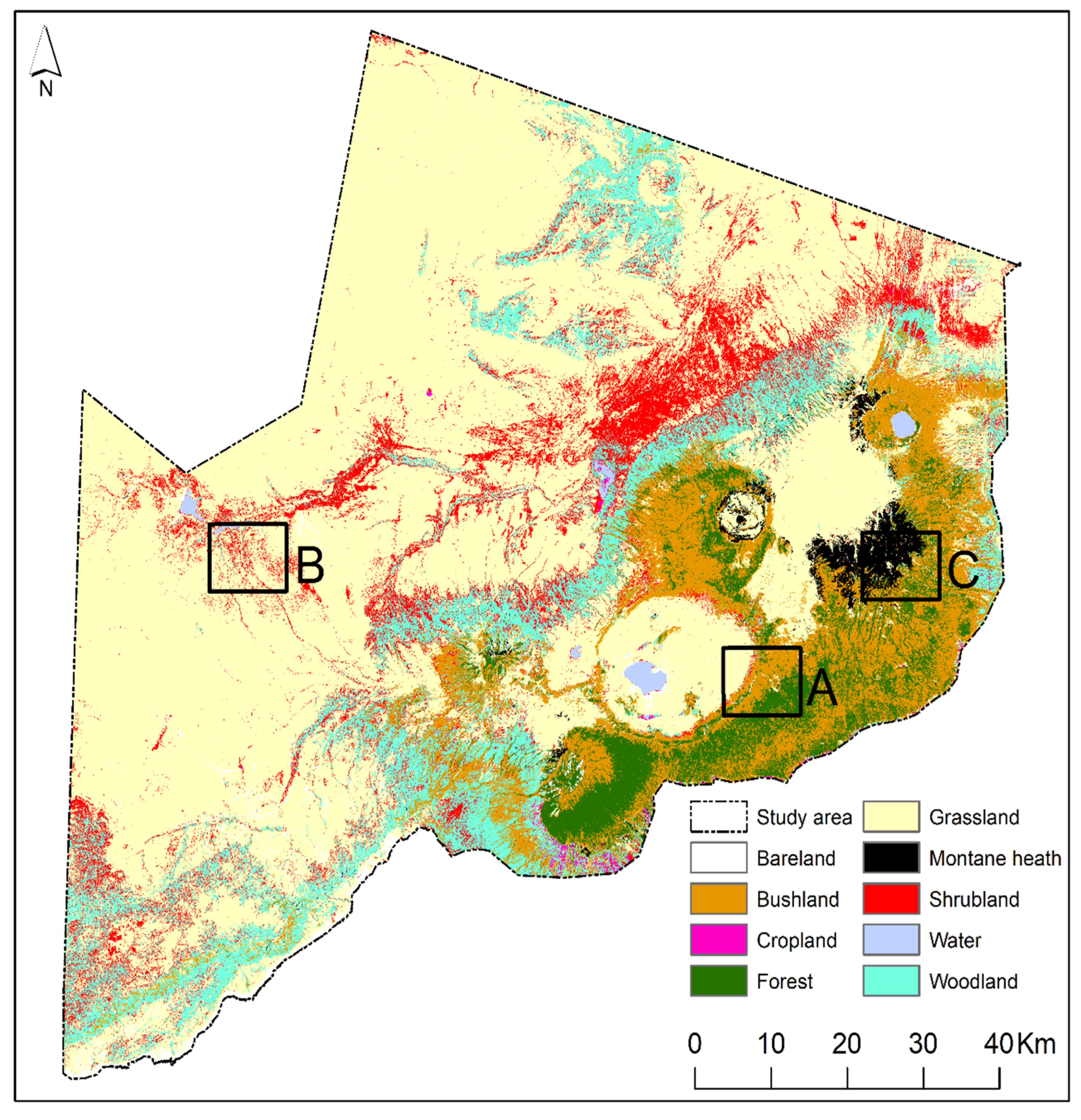
  • Bareland: areas with minimal plant cover that include bare rock, sand, alpine snow and ice, saline or alkaline flats or riverine deposits. These areas often experience extreme environmental conditions, such as low rainfall, high winds, high salinity and toxic or infertile soils that prevent vegetation from developing.
  • Bushland: areas of woody plants, bushes or trees, with a closed shrub canopy between 3 and 6 m in height. The closed canopy of bushland thicket has little grazing value and makes it challenging for large animals to navigate through [49].
  • Cropland: areas where natural vegetation has been removed or modified and replaced by other types of vegetation that requires human activity to maintain it in the long term. Cropland fields may be fallow at certain times during the year.
  • Forest: areas with closed canopy trees of one or more storeys, rising from 7 to ≥40 m in height. Bushes and shrubs dominate the ground making it difficult for animals to travel through it.
  • Grassland: areas dominated by grasses <25 to 150 cm tall, sometimes with herbs, scarred trees or shrubs, with a high grazing value for both wildlife and livestock. Areas may contain some woody cover and may be almost bare during the dry season and during drought episodes.
  • Montane heath: areas with medium sized woody vegetation (<1 m) that can be shrubs, grasses, ferns and mosses. Montane heath occurs in environments ≥600 m in altitude, usually on mountains, but also on hills with lower and more variable temperatures and rainfall.
  • Shrubland: areas with medium sized woody vegetation (<6 m in [49]), generally open canopy, surrounded by grassland or dry land. Some occasional trees and bushes are present depending on location.
  • Water: areas that can be lakes, rivers, ponds or reservoirs, which vary with season.
  • Woodland: tree-covered area with trees as tall as 20 m and an open canopy surrounded by grassland and sometimes shrub but not thicket. These areas are sometimes dominated by only a few species of trees.

3. Materials and Methods

We combined SAR (Sentinel-1) and optical (Sentinel-2) data from three different seasons (dry, wet and short-dry seasons) and compared the outcomes to optimise land cover mapping in savannahs. Sentinel-2 data were obtained and processed in the Framework for Operational Radiometric Correction for Environmental monitoring (FORCE) software version v.2.0 and three Best Available Pixel composites were created for each targeted season [35]. The NDVI bands were also calculated and added. The Google Earth Engine computing platform was used to acquire, process and calculate the textural metrics for Sentinel-1 data for the three target seasons [50,51]. Training data were collected based on our knowledge of the area and Google Earth (Digital Globe) imagery. The land cover classifications were produced using random forests (RF; [52]) and validated with a two-stage random sampling procedure according to best practice guidelines [53]. Figure 2 is a flowchart of our methodological framework.

3.1. Data

3.1.1. Sentinel-2

Sentinel-2 is an Earth Observation mission from the European Space Agency’s (ESA) Copernicus Programme. It consists of two satellites, Sentinal-2A and Sentinel-2B, launched in 2015 and 2017, respectively [10]. Sentinel-2 carries a Multi-Spectral Instrument (MSI) that images 13 spectral bands in the visible, near infrared and shortwave infrared spectral range (SWIR) at 10–60 m spatial resolution. The combination of Sentinel 2A and 2B provides a 5-day revisit rate. Sentinel-2 imagery are freely available and accessible through the Copernicus API Hub.
We obtained all Sentinel 2 images that intersected our study area between 1 January 2019 and 30 September 2019, with less than 75% cloud cover, resulting in 521 images (Table 1). All image processing was in the Framework for Operational Radiometric Correction for Environmental monitoring (FORCE) software version v.2.0 [35]. Firstly, Level 1C images were downloaded from the Copernicus API hub. Secondly, the raw images were processed to Level 2 using the FORCE L2PS module, applying: atmospheric and topographic correction, cloud and cloud shadow masking, data cubing, and downscaling of the 20 m bands using the ImproPhe algorithm [54,55,56].
Next, we produced three Best Available Pixel Composites using the L3PS module. The temporal windows were chosen according to the general climatological patterns in the study area but also the specific rainfall dynamics for the year of study (i.e., 2019): March to May for the wet season; June to September for the dry season, and January to February for the short-dry season (Table 1). These composites score all available observations within the temporal window selecting the optimal observation based on nonparametric quality scoring. The final products included three composites with 10 bands each to which a normalised difference vegetation index (NDVI) band was then calculated and added.

3.1.2. Sentinel-1

Sentinel-1 is an Earth Observation mission from ESA’s Copernicus Programme consisting of two satellites, Sentinal-1A and Sentinel-1B, launched in 2014 and 2016, respectively [10]. Sentinel-1 carries a C-band Synthetic-aperture radar (SAR), which is unaffected by clouds and has been successfully employed in savannah environments for mapping land cover characteristics [10,57]. In comparison to the ALOS PALSAR 2 L-band, the C-band is a shorter wavelength with a shallower penetration into open savannah vegetation [31]. The C-band is better at detecting leaves and grasses and therefore more useful for canopy and cropland studies [31]. The L-band is a long wave band more suitable for closed canopy forested environments as it successfully detects woody vegetation [31].
The Google Earth Engine (GEE) computing platform [50,51] was used to process the Sentinel-1 data and to calculate the metrics from the VV and VH bands (25th, 50th, and 90th percentiles and standard deviation). The temporal windows used were the same as for the Sentinel-2 processing. The final products consisted of three composites, one for each season, with eight bands each.

3.2. Classification Strategy

3.2.1. Training Samples and Classification

The training data were collected based on our knowledge of the area and high-resolution Google Earth (Digital Globe) imagery acquired between 2013 and 2019. A total of 4430 training points were used (306 for ‘Bareland’; 397 for ‘Bushland’; 320 for ‘Cropland’; 370 for ‘Forest’; 1093 for ‘Grassland’; 337 for ‘Montane heath’; 580 for ‘Shrubland’; 301 ‘Water’ and 726 for ‘Woodland’).
Classifications were carried out in the R statistical Software Environment, using the ‘RStoolbox’ and ‘randomforest’ packages [58,59]. The land cover maps were created using the ‘SuperClass’ function [58] and random forests (RF; [52]). RF is a nonparametric machine learning classifier, that combines decision trees with bootstrapping and aggregation [28,52,60,61]. It has been proven to be more time effective and highly accurate in comparison to traditional approaches, such as maximum likelihood, and support vector machines (SMV) [60,61]. RF was implemented using the ‘SuperClass’ function, which takes as an input, the training data and the corrected Landsat image [58]. Specifically in African savannahs, RF classification has successfully been applied in southern Africa [29,36,37,38] and eastern Africa [62,63].

3.2.2. Modelling Framework: Season and Sensor Combinations

In order to determine the best sensor and seasonal combinations to map savannah landscapes, we developed 21 models consisting of combinations of three seasons using Sentinel-1 and 2 imagery (Table 2).

3.2.3. Validation and Accuracy Assessment

The final classified maps were validated using a two-stage random sampling procedure as recommended the best practice guidelines [53]. First, an initial sample of 675 points (75 per class) was randomly obtained from the classified map with the preliminary higher overall accuracy (Model 4 in Table 2). The accuracy was calculated together with the size of the area covered by each land cover class from the same map (Model 4 in Table 2). The second stage used this information as a basis for identifying a suitable validation sample size. The final validation samples were 2147 in total, covering seven classes: 82 for ‘Bareland’; 218 for ‘Bushland’; 103 for ‘Forest’; 1262 for ‘Grassland’; 56 for ‘Montane heath’; 184 for ‘Shrubland’; 242 for ‘Woodland’. The area covered by the ‘Water’ and ‘Cropland’ classes was too small and, therefore, they were not considered in the validation process.
Following the validation, the accuracy assessment was determined by calculating the following statistics: the overall accuracy, user’s accuracy and producer’s accuracies. A nonparametric McNemar’s test was carried out to determine if there were statistically significant differences between the classifications performance [64].

4. Results

4.1. Sentinel-2 and Sentinel-1 Seasonal Imagery to Map Savannah Land Cover Types

The multisensor and multiseason model, incorporating Sentinel-1 and Sentinel-2 data for both the dry and the short-dry season (Model 18) was the best preforming model, with an overall accuracy of 86.3 ± 1.5% (Figure 3 and Figure 4). A land cover map produced from this model is shown in Figure 3, with the associated confusion matrix and accuracy statistics in Table 3. Adjusting the mapped areas, using stratified area estimation, identified ‘Grassland’ as the predominant land cover type covering 60% of the study area (5631 ± 106 km2), followed by ‘Woodland’ (1205 ± 90 km2), ‘Shrubland’ (922 ± 111 km2) and ‘Bushland’ (842 ± 63 km2). Smaller classes comprised the remaining 8% of the NCA, with ‘Forest’ accounting for 5% (507 ± 44 km2), and ‘Bareland’ and ‘Montane heath’ combined covering 3% (276 ± 30 km2).
Models 4, 7, 16, 20 and 21 all achieved accuracies greater than 85%, using different season and sensor combinations (Table 2, Table S1, Figure 4). These five models, and the best-performing model, were able to map the majority of the savannah vegetation types, with the exception of ‘Shrubland’ (Figure 5 and Figure 6, Table S2), with comparable accuracies.
In all models, the most reliably mapped class was ‘Grassland’, with maximum producer’s and user’s accuracies of 96% and 92%, respectively, achieved by Model 21 (Figure 5 and Figure 6). The accuracy of the remaining six classes varied considerably in several models. ‘Shrubland’, for instance, was mapped poorly by all models, with a maximum user’s and producer’s accuracy of 59% and 54%, respectively, achieved by Model 16. The ‘Forest’ class was mapped accurately by Sentinel-2 or multisensor models (e.g., Models 7 and 18). However, Sentinel-1-only models were unable to map it successfully scoring a maximum user’s accuracy of 38% and producer’s accuracy of 33% achieved by Model 11 (Figure 5 and Figure 6). The remaining classes, namely ‘Bushland’, ‘Woodland’, ‘Shrubland’ and ‘Montane heath’ were also mapped more accurately by Sentinel-2 and multisensor models than by the Sentinel-1-only models.

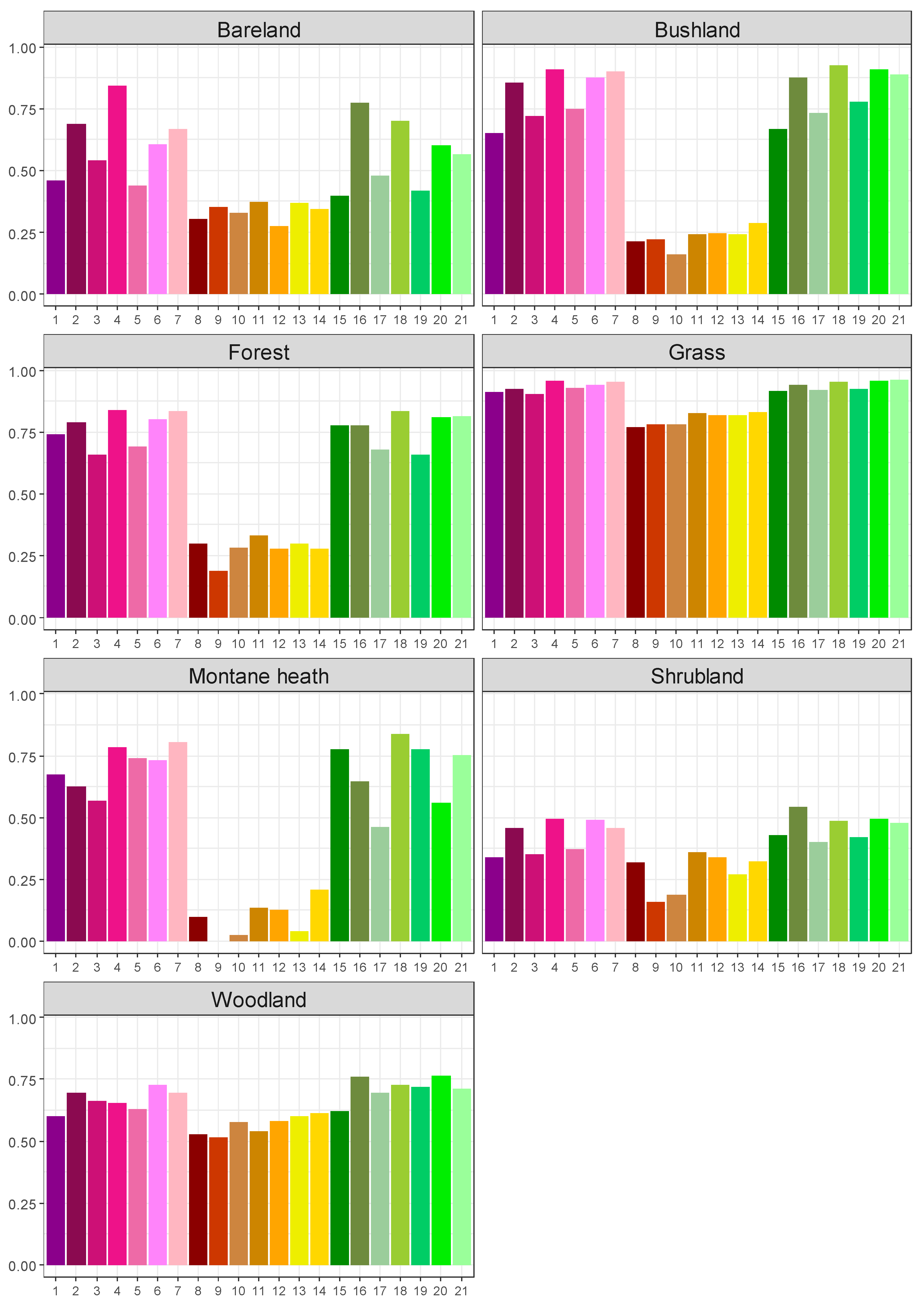
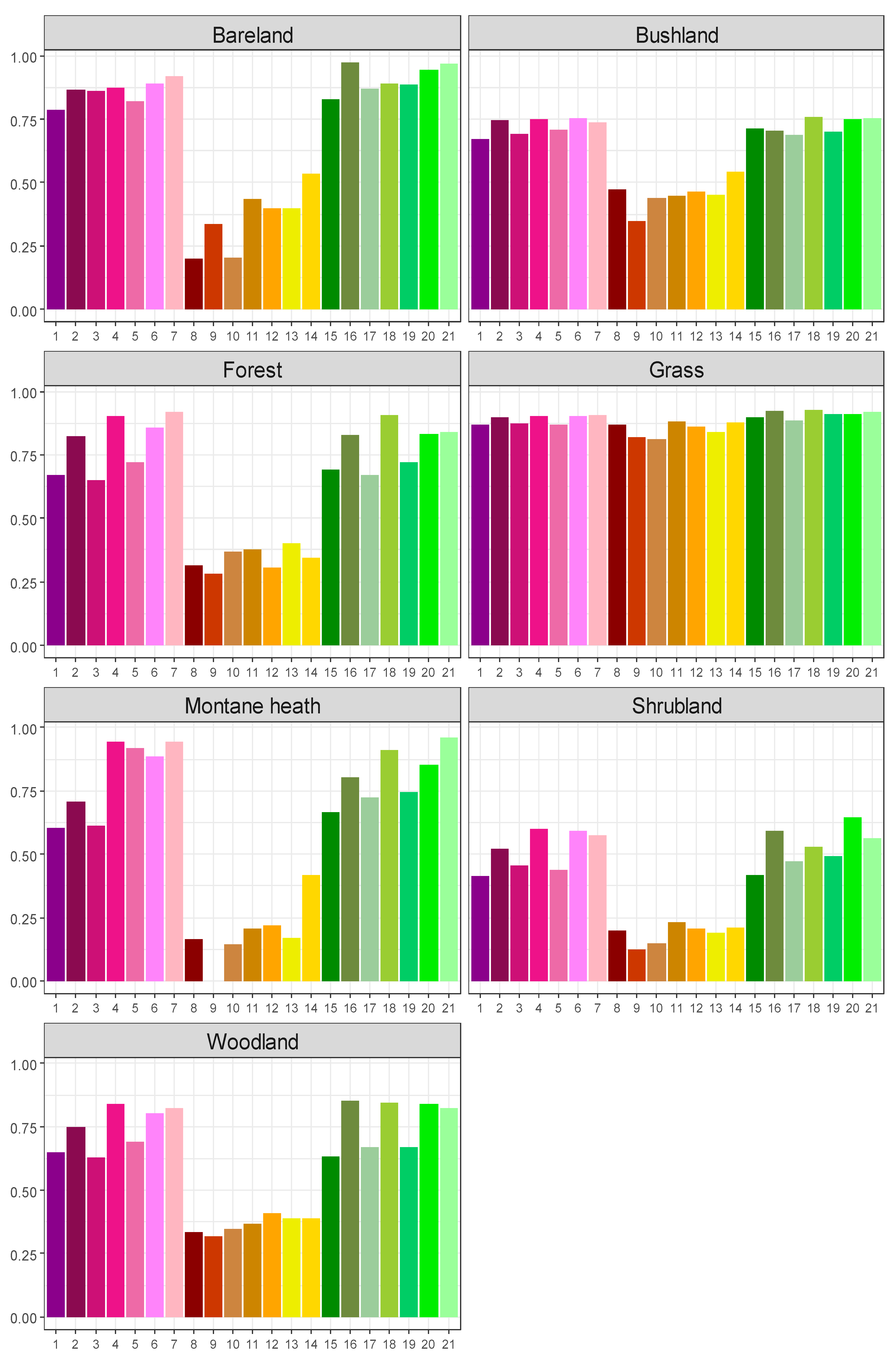
4.2. The Role of C-Band SAR

Comparing the two different sensors, Sentinel-2 models outperform the Sentinel-1 ones, in all combinations and land cover types (Figure 4). Sentinel-1 models have much lower overall accuracies and fail to distinguish most land cover types well, especially ‘Montane heath’, which goes completely undetected in Model 9 (Figure 5 and Figure 6). In terms of the spatial configuration of the classified land cover maps, those produced by the Sentinel-1 models also show a higher degree of confusion between ‘Woodland’, ‘Bushland’ and ‘Forest’, and tend to overestimate ‘Shrubland’ (Figure 7(A4, B4 and C4)). ‘Grassland’ was the only land cover type that Sentinel-1-only models were able to identify with higher accuracies (>76.8%; Model 10; Figure 5 and Figure 6). When combining Sentinel-2 and Sentinel-1 data, all models scored higher overall accuracies when compared to their single sensor counterparts (Figure 4). For example, the overall accuracy of Model 2 (i.e., Sentinel-2-only, short-dry season) increased from 82.7% (±1.6%) to 85.7% (±1.5%) after the Sentinel-1 data were added (Figure 4; McNemar test: p < 0.05).
For single season models, adding radar data improved accuracies for nearly all land cover types, with few exceptions (Figure 5 and Figure 6). For instance, adding Sentinel-1 data to the short-dry single-season (Model 2), increased the accuracy for most land cover types, except for the user’s accuracy of ‘Bushland’ and producer’s accuracy for ‘Forest’ (Figure 5 and Figure 6). For multiseason models, adding Sentinel-1 data only improved the overall accuracy slightly (Figure 4), and visually the land cover maps are very similar (Figure 7(A1–C1,A3–C3)). For instance, the overall accuracy for Model 4 (i.e., Sentinel-2, dry and short-dry seasons) increased slightly from 85.5% (±1.5%) to 86.3% (±1.5%) after the Sentinel-1 data were added; however, this increase is within the respective confidence interval and is statistically insignificant (Figure 4; McNemar test: p > 0.05). Moreover, adding the SAR data to Model 4 decreased the producer’s accuracy for ‘Bareland’, ‘Grassland’, ‘Forest’ and ‘Shrubland’ and decreased the user’s accuracy for ‘Shrubland’ and ‘Montane heath’ (Figure 5 and Figure 6). This decrease in the per-class accuracies for some land cover types occurs in other models, too: when adding Sentinel-1 data to Model 7 (which combines all three seasons; Figure 5 and Figure 6), a decrease in the producer’s accuracy for ‘Bareland’, ‘Bushland’, ‘Forest’ and ‘Montane heath’ and a decrease in the user’s accuracy for ‘Forest’ and ‘Shrubland’ is observed.

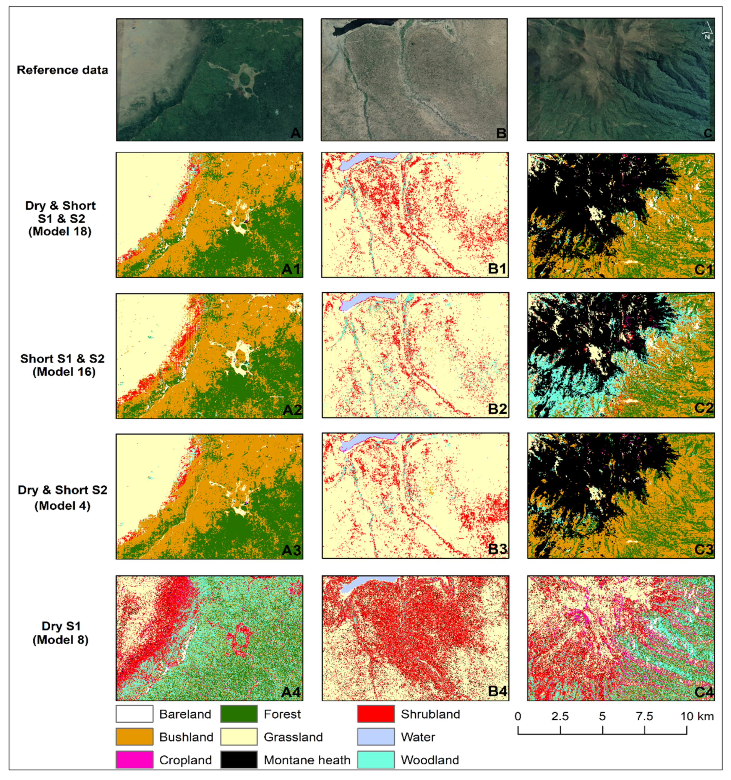
4.3. The Role of Season

Unlike their Sentinel-1 counterparts, Sentinel-2 single season models with data from the short-dry season out-performed dry or wet mono-season ones (Figure 4 and Figure 8). Additionally, all single season models, using dry or wet season imagery, produced very similar overall accuracies (e.g., Model 1 obtained 77.3% and Model 3 obtained 77.8% (McNemar test: p > 0.05); Figure 4 and Figure 8). Both Sentinel-2 and multisensor models incorporating the short-dry season, on its own or with other seasons, performed better than other combinations (Figure 4 and Figure 8; McNemar test: p < 0.05). In Sentinel-2-only models, combining the short-dry season with either the wet or dry seasons, improved all land cover classes, except for the producer’s accuracy for ‘Bareland’, in Model 6 and ‘Woodland’, in Model 4, which performed better with the short-dry season on its own (Figure 5 and Figure 6). Regarding the SAR-only models, season does not seem to have a clear effect on overall accuracies (Figure 4 and Figure 8). However, when optical and SAR data were combined, the models that incorporated the short-dry season, obtained overall accuracies >85.6%—this included the best performing model (Model 18; Figure 4 and Figure 8).
Combining imagery from more than one season increased model accuracy (Figure 4 and Figure 8). For Sentinel-2-only models, using only the dry and short-dry seasons produced accuracies of 77.3 ± 1.8% and 82.7 ± 1.6%, respectively, while a combination of both, increased the accuracy by 2.8% (to 85.5 ± 1.5%; Figure 4 and Figure 8; McNemar test: p < 0.05). In addition, this combination obtained similar results to the best performing model (Figure 7(A1–C1,A3–C3)). For Sentinel-1-only models, the dry and short-dry season models produced accuracies of 58.5% (±2.1%) and 57.6% (±2.1%), respectively; when combined this rises to 63.7 ± 2.1% (Figure 4 and Figure 8; McNemar test: p < 0.05).
The models that combined more than one season scored lower commission and omission errors for most land cover classes (Figure 5 and Figure 6). For Sentinel-2-only models, the combination of dry and short-dry seasons (i.e., Model 4), increased the accuracy for most land cover types, with the exception of the producer’s accuracy of ‘Woodland’ (Figure 5 and Figure 6). In addition, the combination of wet and short-dry season (Model 6) increased the accuracy for nearly all land cover types, except for the producer’s accuracy of ‘Bareland’ (Figure 5 and Figure 6). On the other hand, for multisensor models, combining more than one season increased overall accuracies slightly but these varied depending on the land cover type. For instance, the combination of dry and short-dry season data in multisensor models (Models 15 and 16) decreased the user’s accuracy for ‘Bareland’ by 8%, of ‘Shrubland’ by 6%, of ‘Woodland’ by 1% and of ‘Bushland’ by 5%. Producer’s accuracy also decreased for ‘Bareland’ (7%), ‘Shrubland’ (6%) and ‘Woodland’ (3%; Figure 5 and Figure 6). Despite the statistics, there are areas where the opposite holds true, as in the case of the mountains northeast of the Crater (Figure 7C). In that area the inclusion of the dry season data corrected the wrongly classified ‘Woodland’ for ‘Bushland’ (Figure 7(C1,C2)).
Interestingly, the combination of all three seasons did not significantly improve the overall accuracy for most of the models (McNemar test: p > 0.05). However, this combination performed better than the combination of data from the dry and wet seasons (Figure 4 and Figure 8; McNemar test: p < 0.05). Nonetheless, the three-season models seem to be beneficial for the mapping of specific land cover classes (Figure 5 and Figure 6). Considering only the Sentinel-2 models, the three-season combination increases the user’s accuracy for ‘Forest’, ‘Bareland’ and ‘Grassland’ and increases the producer’s accuracy for ‘Montane heath’, when compared to single- or biseason combinations (Figure 5 and Figure 6).

5. Discussion

5.1. Can Sentinel-2 and Sentinel-1 Seasonal Imagery Be Used to Accurately Map Savannah Land Cover Types at the Regional Scale?

To improve habitat monitoring, preserve biodiversity and sustain ecosystem services, the provision of moderate-resolution land cover maps across savannah environments is essential. Mapping savannahs is a challenging task, due to varying vegetation densities, high background soil signal, and the spectral similarities between the dominant land cover types [10,24,25]. Our results demonstrate that imagery from the Sentinel constellation (optical and C-band SAR) has good utility for mapping complex savannah systems at moderate resolution. Our best performing model—using a combination of Sentinel-2 and Sentinel-1 data from the dry and short-dry seasons—achieved an overall accuracy of 86.3 ± 1.5%. This compares favourably with other studies in savannah environments (e.g., [10,28,29,37]). The land cover type most accurately mapped was ‘Grassland’ obtaining a maximum producer’s and user’s accuracy of 96% and 92%, respectively, achieved by Model 21 (three seasons). This is consistent with previous research (Figure 5 and Figure 6, [28]). On the other hand, the performance of ‘Shrubland’ was relatively poor, scoring a maximum user’s accuracy of 59% and producer’s accuracy of 54%, achieved by Model 16 (Figure 5 and Figure 6). A study carried out by Mishra (2014; [37]) found that lower vegetation density/height, such as ‘Shrubland’, performed poorly at finer scales. Spectral similarities, similar ecological composition and the fact that ‘Shrubland’ vegetation is highly variable and difficult to identify using Google Earth imagery, can also explain the confusion between ‘Shrubland’, ‘Woodland’ and ‘Grassland’ [65]. To investigate the reliability of mapping savannahs using Sentinel imagery that comes with an undisputed spatial resolution advantage compared to Landsat or MODIS, we examined the role of different sensor and season combinations on mapping accuracies.

5.2. Can the Combination of Optical and Radar Data Improve Classification Accuracies?

Our results show models using solely Sentinel-1 data underperformed their Sentinel-2 counterparts, for all seasons and all land cover types (Figure 4). The best Sentinel-2 only model (dry and short-dry season) produced an 85.5% overall accuracy compared to 64.7% for the best Sentinel-1 only model (all seasons): a nontrivial difference (McNemar test: p < 0.05). This agrees with both Lopes et al. (2019; [66]) and Higginbottom et al. (2018; [29]) who compared optical with radar imagery in West and South Africa, respectively. This could be attributed to SAR-only models incurring errors caused by incidence angle variation, speckle, geolocation accuracy and moisture content [29]. The results from Naidoo et al. (2016; [30]) who mapped woody vegetation cover in southern African savannahs show the opposite result, but they employed longer wavelength L-band data (ALOS PALSAR), which are more sensitive to the dense woody vegetation structure [25,28,29].
The SAR-only models were able to successfully identify only the ‘Grassland’ land cover type (accuracies above 76.8%). ‘Montane heath’ on the other hand, obtained accuracies as low as 0% in Model 9 and was often confused for ‘Grassland’, likely due to textural similarities between the two land cover types and their lack of dense or woody plants. Interestingly, the woody classes also scored low accuracies in the SAR-only models, with open ‘Woodland’ achieving a maximum of 57.5% (Model 10), ‘Bushland’ 47.2% (Model 8) and closed ‘Forest’ 37% (Model 10) (Figure 5 and Figure 6). The relatively large number of woody classes in our study area and the land cover nomenclature we adopted might explain the confusion between them, as previous research shows that combining such classes can improve mapping accuracy from SAR data [67,68]. In addition, Huttich et al. (2011; [69]) suggested that using inter-annual metrics of over one or two years could increase accuracies of ‘Shrubland’ and ‘Grassland’ classes. Our results also show that SAR only models overestimated ‘Shrubland’, specifically in low vegetated areas (Figure 7(A4–C4)). This can be attributed to the high surface roughness that produces similar signals for trees and shrubs [10,70]. Zhang et al. (2019; [10]) and Urban et al. (2020; [70]), also showed that radar data overestimate the presence of woody vegetation, for the Sahel and South Africa, respectively.
Previous research recommends combining SAR with optical data for improved land cover mapping [10,28,67]. Our results show that the combination of Sentinel-2 and Sentinel-1 data achieves higher overall accuracies when compared to single sensor models. Model 2 (Sentinel-2, short-dry season), scored an overall accuracy of 82.7%, increased by 3% when Sentinel-1 data were added (Figure 4; McNemar test: p < 0.05). The addition of SAR data increased the accuracies for most vegetation types, with the UA for ‘bushland’ and PA of closed ‘forest’ being the only two exceptions. These results are consistent with previous research carried out by Laurin et al. (2013; [67]) and Symeonakis et al. (2018; [28]), finding that combining SAR and optical data also decreased the omission and commission errors for all land cover types. Zhang et al. (2019; [10]) suggested adding SAR to optical data as they can correct errors particularly in highly productive areas (e.g., wetlands, irrigated fields and perennial grasses) which can be misclassified as trees.
Our findings agree with the emerging consensus that multisensor approaches to land cover mapping perform best. However, we found the benefits of multisensor approaches were most evident in mono-temporal models. For instance, adding SAR data to Model 4 (Sentinel-2 data, dry and short-dry seasons), improved its overall accuracy by only 0.8% (Figure 4; McNemar test: p > 0.05). This slight increase is within the confidence interval of both models (Models 4 and 18) and produce a very similar spatial configuration of the mapped land cover classes (Figure 7(A1–C1,A3–C3)). Our results, therefore, support those of Higginbottom et al. (2018; [29]), who found that the multisensor approach was only marginally beneficial (≈1%), and at fine scales (30m) the addition of PALSAR data to Landsat may reduce accuracies. Chatziantoniou et al. (2017; [71]) achieved similar results to ours, suggesting that although SAR data are solely impacted by wind, droughts might also influence the data quality thereby negatively affecting the overall classification accuracy. Therefore, if multiseason data is available, combining more than one sensor might be unnecessary and even counterproductive for specific land cover types (e.g., ‘Shrubland’).

5.3. How Does the Combination of Data from Different Seasons Influence the Accuracy of the Classification?

Savannah mapping studies generally use data from the dry season, due to significantly lower cloud contamination and heightened contrasts between woody and grassland components [29,32]. We found only small differences in accuracy, less than 1%, between wet and dry season models, for Sentinel-2 and multisensor scenarios (Figure 4 and Figure 8; McNemar test: p > 0.05), which agrees with Symeonakis et al. (2018; [29]). Interestingly, Sentinel-2 imagery from the short-dry season, which occurs between January and February was highly effective, preforming comparably to the multisensor models and outperforming the other single season Sentinel-2 models by 5% (Figure 8). The short-dry season, which occurs right after the short rains (from October to December), is characteristic of East Africa and, to our knowledge, this is the first study to examine its utility in mapping savannahs. This season is particularly useful for land cover mapping due to it having cloud free data and being wet enough for herbaceous vegetation to be photosynthetically active, which is not the case during the dry season [33]. In the Ngorongoro Conservation Area (NCA), during the short-dry season the grasses in the North-West of the NCA starts to emerge, attracting the great wildebeest migration. Moreover, this season is dry enough to provide noticeable differences in the spectral characteristics of woody and herbaceous vegetation [30].
We found that models combing dry and wet season imagery outperform their single season counterparts in all scenarios (Figure 8). However, compared to other model combinations, Sentinel-2-only and multisensor models were improved by including the short-dry season data (Figure 8). The dry season (Model 1) and the short-dry season model (Model 2) produced an overall accuracy of 77.3% and 82.7%, respectively. Once combined, the overall accuracy increased to 85.5% (≈2.8%, McNemar test: p < 0.05), which is very close to the best performing model (Figure 4; McNemar test: p > 0.05). This agrees with Haro-Carrión and Southworth (2018; [32]) and Symeonakis et al. (2018; [28]), who also reported higher accuracies when combining biseasonal data. Adding multiseason data provides additional spectral information and, if available, should be preferred for successfully distinguishing between spectrally similar savannah vegetation classes [32].
Multiseason models generally scored higher overall accuracies; however, multisensor models were less improved. For instance, the increase in the overall accuracy from the combination of Models 15 and 16, which include multisensor data for the dry and short-dry seasons, was ≈0.6% (p > 0.0.5). This agrees with Symeonakis et al. (2018; [28]) who reported the same increase of 0.6% in the overall accuracy for their multisensor dry season model by combining sensors and seasons. Regardless of the impact on the overall accuracy, our results show that adding more than one season to multisensor models solved misclassification problems in specific areas within the NCA (Figure 7). For instance, in the mountains northeast of the Crater (Figure 7C), Model 16 overestimated the open ‘Woodland’ cover: by adding the dry season data, the classification was improved (Figure 7(C1,C2)). These errors in the spatial configuration of the mapped classes can go unnoticed, as the calculation of accuracy statistics is carried out over a limited number of locations compared to the much larger total number of pixels of the study area.
Most multiseason mapping studies consider only the wet and dry seasons or a combination of the two. Our results show that the triseasonal models performed better than the wet and dry season models (McNemar test: p < 0.05) and improved the accuracies for several specific land cover types (e.g., closed ‘Forest’ and ‘Grassland’ achieved 92% and 90.6%, respectively, in Model 7). However, the overall accuracy did not increase significantly when compared to other biseasonal models. For example, Model 21 (three seasons) achieved an overall accuracy of 85.6%, which is higher than Model 19 (dry and wet; 81.2%, McNemar test: p < 0.05), but (insignificantly) lower than Model 18 (dry and short-dry; 86.3%, McNemar test: p > 0.05) (Figure 4 and Figure 8). These results contrast with Hüttich et al. (2011; [69]) who found that increasing the length of the observation period and interseasonal data increases the accuracy of the classification. However, the scholars also mention that highly dynamic classes, such as ‘Grassland’ and ‘Bareland’, benefit when longer time series are used which our results support. Whilst there are benefits from using triseasonal imagery, it must be noted that the amount of data and time required for preprocessing also increases significantly. Unless triseasonal data provide improvements for mapping specific vegetation types of interest, using a combination of the dry and short-dry seasons should suffice.

5.4. Implications for Biodiversity Monitoring/Ecosystem Monitoring Challenges in the Area

This study has demonstrated that Sentinel imagery can reliably map land cover in the Ngorongoro Conservation Area (NCA), and the wider Serengeti region. The NCA is globally important for biodiversity conservation due to the presence of iconic megafauna, such as the Eastern black rhino and African elephant. It is among the best locations in the world to see black rhino in the wild, attracting thousands of tourists every year. The NCA supports the largest black rhino population in Tanzania and in recent years this population increased to 56 individuals [72]. Currently, there is emerging evidence of a decrease in the quality and quantity of preferable browse and, consequently, a decrease in suitable habitat for black rhino [14,41,73]. Unsuitable habitats and limited browse promote intra- and interspecific competition for resources and emigration of rhinos out of the Crater and the NCA [73]. Our derived land cover map could help monitor black rhino habitat quality and identify new locations within the NCA which the population could expand into. In addition, land cover maps can infer rhino home ranges and support antipoaching efforts in the NCA. Previously, the only detailed land cover survey in the NCA was completed in 1972 [45], before several major management policies were introduced that brought about significant environmental changes, e.g., the displacement of pastoralists from the Ngorongoro Crater [14,46]. Therefore, our accurate and up-to-date land cover map could have considerable conservation implications for the NCA, in general, and the black rhino population, in particular, as it provides information essential for the development of sustainable management strategies.

6. Conclusions

Savannahs are heterogeneous environments providing essential ecosystem services to communities. Currently, they are threatened by extensive land use/cover changes and subsequent land degradation. Mapping these environments is challenging but essential in order to improve monitoring capabilities, prevent biodiversity loss and ensure savannah ecosystem service provision. In this study, we tested how combinations of imagery from different seasons and sensors affects the accuracy of land cover maps for the NCA and provide guidance for future attempts to monitor and understand savannah landscapes. We conclude that the combination of Sentinel-1 and 2 data from the dry and short-dry seasons successfully maps most of the land cover types in the NCA, with ‘Shrubland’ remaining a challenge. Additionally, we found that if SAR data are unavailable, multiseason Sentinel-2 data provide a good alternative, whilst if no multiseasonal data can be used, a combination of SAR and optical data can be used to accurately map savannah environments with similar results to the best performing model. Finally, we advise that the short-dry season should be preferred over the wet and dry seasons for both multisensor combinations and optical data. In conclusion, we provide much needed and highly accurate, medium resolution land cover maps for the NCA, which will support sustainable management and conservation.

Supplementary Materials

The following are available online at https://www.mdpi.com/2072-4292/12/23/3862/s1, Table S1: Overall accuracy of the models tested, Table S2: User’s and producer’s accuracy of all land cover types and models tested.

Author Contributions

Conceptualisation, J.B. and E.S.; Formal analysis, J.B.; Methodology, J.B., T.P.H. and E.S.; Project administration, E.S. and M.J.; Supervision, E.S. and M.J.; Validation, J.B., T.P.H. and E.S.; Writing—original draft, J.B., T.P.H. and E.S.; Writing—review and editing, M.J. All authors have read and agreed to the published version of the manuscript.

Funding

This research received no external funding and the APC was funded by the Ecology and Environment Research Centre (EERC) of Manchester Metropolitan University.

Conflicts of Interest

The authors declare no conflict of interest.

References

  1. Solbrig, O.T. The diversity of the savanna ecosystem. In Biodiversity and Savanna Ecosystem Processes; A Global Perspective; Springer: Berlin/Heidelberg, Germany, 1996; Volume 121, pp. 1–27. [Google Scholar]
  2. Liu, Y.Y.; van Dijk, A.; de Jeu, R.A.M.; Canadell, J.G.; McCabe, M.F.; Evans, J.P.; Wang, G.J. Recent reversal in loss of global terrestrial biomass. Nat. Clim. Chang. 2015, 5, 470–474. [Google Scholar] [CrossRef]
  3. Pfeifer, M.; Platts, P.J.; Burgess, N.D.; Swetnam, R.D.; Willcock, S.; Lewis, S.L.; Marchant, R. Land use change and carbon fluxes in East Africa quantified using earth observation data and field measurements. Environ. Conserv. 2013, 40, 241–252. [Google Scholar] [CrossRef] [Green Version]
  4. Poulter, B.; Frank, D.; Ciais, P.; Myneni, R.B.; Andela, N.; Bi, J.; Broquet, G.; Canadell, J.G.; Chevallier, F.; Liu, Y.Y.; et al. Contribution of semi-arid ecosystems to interannual variability of the global carbon cycle. Nature 2014, 509, 600–603. [Google Scholar] [CrossRef] [PubMed] [Green Version]
  5. Schneibel, A.; Frantz, D.; Roder, A.; Stellmes, M.; Fischer, K.; Hill, J. Using Annual Landsat Time Series for the Detection of Dry Forest Degradation Processes in South-Central Angola. Remote Sens. 2017, 9, 905. [Google Scholar] [CrossRef] [Green Version]
  6. Symeonakis, E.; Higginbottom, T. Bush encroachment monitoring using multi-temporal Landsat data and Random Forests. In Proceedings of the International Archives of the Photogrammetry, Remote Sensing and Spatial Information Sciences—2014 ISPRS Technical Commission II Symposium, Toronto, ON, Canada, 6–8 October 2014; Volume XL-2, pp. 29–35. [Google Scholar] [CrossRef] [Green Version]
  7. Eldridge, D.J.; Bowker, M.A.; Maestre, F.T.; Roger, E.; Reynolds, J.F.; Whitford, W.G. Impacts of shrub encroachment on ecosystem structure and functioning: Towards a global synthesis. Ecol. Lett. 2011, 14, 709–722. [Google Scholar] [CrossRef]
  8. Stevens, N.; Lehmann, C.E.R.; Murphy, B.P.; Durigan, G. Savanna woody encroachment is widespread across three continents. Glob. Chang. Biol. 2017, 23, 235–244. [Google Scholar] [CrossRef] [PubMed] [Green Version]
  9. Venter, Z.S.; Cramer, M.D.; Hawkins, H.J. Drivers of woody plant encroachment over Africa. Nat. Commun. 2018, 9, 2272. [Google Scholar] [CrossRef] [Green Version]
  10. Zhang, W.; Brandt, M.; Wang, Q.; Prishchepov, A.V.; Tucker, C.J.; Li, Y.; Lyu, H.; Fensholt, R. From woody cover to woody canopies: How Sentinel-1 and Sentinel-2 data advance the mapping of woody plants in savannas. Remote Sens. Environ. 2019, 234, 111465. [Google Scholar] [CrossRef]
  11. Berthrong, S.T.; Pineiro, G.; Jobbagy, E.G.; Jackson, R.B. Soil C and N changes with afforestation of grasslands across gradients of precipitation and plantation age. Ecol. Appl. 2012, 22, 76–86. [Google Scholar] [CrossRef] [Green Version]
  12. Gray, E.F.; Bond, W.J. Will woody plant encroachment impact the visitor experience and economy of conservation areas? Koedoe 2013, 55. [Google Scholar] [CrossRef] [Green Version]
  13. Angassa, A.; Baars, R.M.T. Ecological condition of encroached and non-encroached rangelands in Borana, Ethiopia. Afr. J. Ecol. 2000, 38, 321–328. [Google Scholar] [CrossRef]
  14. Niboye, E.P. Vegetation Cover Changes in Ngorongoro Conservation Area from 1975 to 2000: The Importance of Remote Sensing Images. Open Geogr. J. 2010, 3, 15–27. [Google Scholar] [CrossRef] [Green Version]
  15. Fritz, H.; Duncan, P. On the carrying-capacity for large ungulates of African savanna ecosystems. Proc. R. Soc. B-Biol. Sci. 1994, 256, 77–82. [Google Scholar] [CrossRef]
  16. Beale, C.M.; van Rensberg, S.; Bond, W.J.; Coughenour, M.; Fynn, R.; Gaylard, A.; Grant, R.; Harris, B.; Jones, T.; Mduma, S.; et al. Ten lessons for the conservation of African savannah ecosystems. Biol. Conserv. 2013, 167, 224–232. [Google Scholar] [CrossRef]
  17. Newmark, W.D. Isolation of African protected areas. Front. Ecol. Environ. 2008, 6, 321–328. [Google Scholar] [CrossRef]
  18. IUCN & UNEP. The World Database on Protected Areas (WDPA); UNEP-WCMC: Cambridge, UK, 2009. [Google Scholar]
  19. Eisfelder, C.; Kuenzer, C.; Dech, S. Derivation of biomass information for semi-arid areas using remote-sensing data. Int. J. Remote Sens. 2012, 33, 2937–2984. [Google Scholar] [CrossRef]
  20. Yang, J.; Prince, S.D. Remote sensing of savanna vegetation changes in Eastern Zambia 1972–1989. Int. J. Remote Sens. 2000, 21, 301–322. [Google Scholar] [CrossRef]
  21. Adole, T.; Dash, J.; Atkinson, P.M. A systematic review of vegetation phenology in Africa. Ecol. Inform. 2016, 34, 117–128. [Google Scholar] [CrossRef]
  22. Woodcock, C.E.; Allen, R.; Anderson, M.; Belward, A.; Bindschadler, R.; Cohen, W.; Gao, F.; Goward, S.N.; Helder, D.; Helmer, E.; et al. Free access to Landsat imagery. Science 2008, 320, 1011. [Google Scholar] [CrossRef]
  23. Wulder, M.A.; Masek, J.G.; Cohen, W.B.; Loveland, T.R.; Woodcock, C.E. Opening the archive: How free data has enabled the science and monitoring promise of Landsat. Remote Sens. Environ. 2012, 122, 2–10. [Google Scholar] [CrossRef]
  24. Tsalyuk, M.; Kelly, M.; Getz, W.M. Improving the prediction of African savanna vegetation variables using time series of MODIS products. ISPRS J. Photogramm. Remote Sens. 2017, 131, 77–91. [Google Scholar] [CrossRef] [PubMed] [Green Version]
  25. Müller, H.; Rufin, P.; Griffiths, P.; Siqueira, A.J.B.; Hostert, P. Mining dense Landsat time series for separating cropland and pasture in a heterogeneous Brazilian savanna landscape. Remote Sens. Environ. 2015, 156, 490–499. [Google Scholar] [CrossRef] [Green Version]
  26. Eggen, M.; Ozdogan, M.; Zaitchik, B.F.; Simane, B. Land Cover Classification in Complex and Fragmented Agricultural Landscapes of the Ethiopian Highlands. Remote Sens. 2016, 8, 20. [Google Scholar] [CrossRef] [Green Version]
  27. Morrison, J.; Higginbottom, T.P.; Symeonakis, E.; Jones, M.J.; Omengo, F.; Walker, S.L.; Cain, B. Detecting Vegetation Change in Response to Confining Elephants in Forests Using MODIS Time-Series and BFAST. Remote Sens. 2018, 10, 1075. [Google Scholar] [CrossRef] [Green Version]
  28. Symeonakis, E.; Higginbottom, T.P.; Petroulaki, K.; Rabe, A. Optimisation of Savannah Land Cover Characterisation with Optical and SAR Data. Remote Sens. 2018, 10, 499. [Google Scholar] [CrossRef] [Green Version]
  29. Higginbottom, T.P.; Symeonakis, E.; Meyer, H.; van der Linden, S. Mapping fractional woody cover in semi-arid savannahs using multi-seasonal composites from Landsat data. ISPRS J. Photogramm. Remote Sens. 2018, 139, 88–102. [Google Scholar] [CrossRef] [Green Version]
  30. Naidoo, L.; Mathieu, R.; Main, R.; Wessels, K.; Asner, G.P. L-band Synthetic Aperture Radar imagery performs better than optical datasets at retrieving woody fractional cover in deciduous, dry savannahs. Int. J. Appl. Earth Obs. Geoinf. 2016, 52, 54–64. [Google Scholar] [CrossRef]
  31. Mathieu, R.; Naidoo, L.; Cho, M.A.; Leblon, B.; Main, R.; Wessels, K.; Asner, G.P.; Buckley, J.; Van Aardt, J.; Erasmus, B.F.N.; et al. Toward structural assessment of semi-arid African savannahs and woodlands: The potential of multitemporal polarimetric RADARSAT-2 fine beam images. Remote Sens. Environ. 2013, 138, 215–231. [Google Scholar] [CrossRef]
  32. Haro-Carrion, X.; Southworth, J. Understanding Land Cover Change in a Fragmented Forest Landscape in a Biodiversity Hotspot of Coastal Ecuador. Remote Sens. 2018, 10, 1980. [Google Scholar] [CrossRef] [Green Version]
  33. Brandt, M.; Hiernaux, P.; Tagesson, T.; Verger, A.; Rasmussen, K.; Diouf, A.A.; Mbow, C.; Mougin, E.; Fensholt, R. Woody plant cover estimation in drylands from Earth Observation based seasonal metrics. Remote Sens. Environ. 2016, 172, 28–38. [Google Scholar] [CrossRef] [Green Version]
  34. Griffiths, P.; van der Linden, S.; Kuemmerle, T.; Hostert, P. A Pixel-Based Landsat Compositing Algorithm for Large Area Land Cover Mapping. IEEE J. Sel. Top. Appl. Earth Obs. Remote Sens. 2013, 6, 2088–2101. [Google Scholar] [CrossRef]
  35. Frantz, D. FORCELandsat + Sentinel-2 Analysis Ready Data and Beyond. Remote Sens. 2019, 11, 1124. [Google Scholar] [CrossRef] [Green Version]
  36. Symeonakis, E.; Petroulaki, K.; Higginbottom, T. Landsat-based woody vegetation cover monitoring in southern African savannahs. Int. Arch. Photogramm. Remote Sens. Spat. Inf. Sci. 2016, 41, 563–567. [Google Scholar] [CrossRef]
  37. Mishra, N.B.; Crews, K.A. Mapping vegetation morphology types in a dry savanna ecosystem: Integrating hierarchical object-based image analysis with Random Forest. Int. J. Remote Sens. 2014, 35, 1175–1198. [Google Scholar] [CrossRef]
  38. Hüttich, C.; Gessner, U.; Herold, M.; Strohbach, B.; Schmidt, M.; Keil, M.; Dech, S. On the Suitability of MODIS Time Series Metrics to Map Vegetation Types in Dry Savanna Ecosystems: A Case Study in the Kalahari of NE Namibia. Remote Sens. 2009, 1, 620–643. [Google Scholar] [CrossRef] [Green Version]
  39. Swanson, L.A. Ngorongoro Conservation Area: Spring of Life. Master of Environmental Studies Capstone Projects. Master’s Thesis, University of Pennsylvania, Philadelphia, PA, USA, 2007. [Google Scholar]
  40. Estes, R.D.; Atwood, J.L.; Estes, A.B. Downward trends in Ngorongoro Crater ungulate populations 1986–2005: Conservation concerns and the need for ecological research. Biol. Conserv. 2006, 131, 106–120. [Google Scholar] [CrossRef]
  41. Amiyo, T.A. Ngorongoro Crater Rangelands: Condition, Management and Monitoring. Master’s Thesis, University of Kwazulu-Natal, Durban, South Africa, 2006. [Google Scholar]
  42. Boone, R.B.; Galvin, K.A.; Thornton, P.K.; Swift, D.M.; Coughenour, M.B. Cultivation and conservation in Ngorongoro Conservation Area, Tanzania. Hum. Ecol. 2006, 34, 809–828. [Google Scholar] [CrossRef]
  43. Hunter, F.D.L.; Mitchard, E.T.A.; Tyrrell, P.; Russell, S. Inter-Seasonal Time Series Imagery Enhances Classification Accuracy of Grazing Resource and Land Degradation Maps in a Savanna Ecosystem. Remote Sens. 2020, 12, 198. [Google Scholar] [CrossRef] [Green Version]
  44. Masao, C.A.; Makoba, R.; Sosovele, H. Will Ngorongoro Conservation Area remain a world heritage site amidst increasing human footprint? Int. J. Biodivers. Conserv. 2015, 7, 394–407. [Google Scholar] [CrossRef] [Green Version]
  45. Herlocker, D.J.; Dirschl, H.J. Vegetation of the Ngorongoro Conservation Area, Tanzania; Canadian Wildlife Service: Sackville, NB, Canada, 1972. [Google Scholar]
  46. Mills, A.; Morkel, P.; Amiyo, A.; Runyoro, V.; Borner, M.; Thirgood, S. Managing small populations in practice: Black rhino Diceros bicomis michaeli in the Ngorongoro Crater, Tanzania. Oryx 2006, 40, 319–323. [Google Scholar] [CrossRef] [Green Version]
  47. Homewood, K.M.; Rodgers, W.A. Maasailand Ecology: Pastoralist Development and Wildlife Conservation in Ngorongoro, Tanzania; Cambridge Studies in Applied Ecology and Resource Management; Cambridge University Press: Cambridge, UK, 1991; ISBN 978-0-521-60749-0. [Google Scholar]
  48. Harris, W.E.; de Kort, S.; Bettridge, C.; Borges, J.; Cain, B.; Dulle, H.; Fyumagwa, R.; Gadiye, D.; Jones, M.; Kahana, L.; et al. A Learning Networks approach to resolve conservation challenges in the Ngorongoro Conservation Area. J. Afr. Ecol. 2020, in press. [Google Scholar] [CrossRef]
  49. Pratt, D.J.; Greenway, P.J.; Gwynne, M.D. A Classification of East African Rangeland, with an Appendix on Terminology. J. Appl. Ecol. 1966, 3, 369. [Google Scholar] [CrossRef]
  50. Gorelick, N.; Hancher, M.; Dixon, M.; Ilyushchenko, S.; Thau, D.; Moore, R. Google Earth Engine: Planetary-scale geospatial analysis for everyone. Remote Sens. Environ. 2017, 202, 18–27. [Google Scholar] [CrossRef]
  51. Moore, R.T.; Hansen, M.C. Google Earth Engine: A new cloud-computing platform for global-scale earth observation data and analysis. AGU Fall Meet. Abstr. 2011, 2011, IN43C-02. [Google Scholar]
  52. Breiman, L. Random Forests. Mach. Learn. 2001, 45, 5–32. [Google Scholar] [CrossRef] [Green Version]
  53. Olofsson, P.; Foody, G.M.; Herold, M.; Stehman, S.V.; Woodcock, C.E.; Wulder, M.A. Good practices for estimating area and assessing accuracy of land change. Remote Sens. Environ. 2014, 148, 42–57. [Google Scholar] [CrossRef]
  54. Frantz, D.; Röder, A.; Stellmes, M.; Hill, J. An Operational Radiometric Landsat Preprocessing Framework for Large-Area Time Series Applications. IEEE Trans. Geosci. Remote Sens. 2016, 54, 3928–3943. [Google Scholar] [CrossRef]
  55. Zhu, Z.; Woodcock, C.E. Object-based cloud and cloud shadow detection in Landsat imagery. Remote Sens. Environ. 2012, 118, 83–94. [Google Scholar] [CrossRef]
  56. Frantz, D.; Stellmes, M.; Roder, A.; Udelhoven, T.; Mader, S.; Hill, J. Improving the Spatial Resolution of Land Surface Phenology by Fusing Medium- and Coarse-Resolution Inputs. IEEE Trans. Geosci. Remote Sens. 2016, 54, 4153–4164. [Google Scholar] [CrossRef]
  57. Baumann, M.; Levers, C.; Macchi, L.; Bluhm, H.; Waske, B.; Gasparri, N.I.; Kuemmerle, T. Mapping continuous fields of tree and shrub cover across the Gran Chaco using Landsat 8 and Sentinel-1 data. Remote Sens. Environ. 2018, 216, 201–211. [Google Scholar] [CrossRef]
  58. Leutner, B.; Horning, N.; Schwalb-Willmann, J. RStoolbox: Tools for Remote Sensing Data Analysis. Available online: https://CRAN.R-project.org/package=RStoolbox (accessed on 11 December 2018).
  59. R Core Team R: A Language and Environment for Statistical Computing; R Foundation for Statistical Computing: Vienna, Austria, 2018. Available online: https://www.r-project.org/ (accessed on 25 November 2020).
  60. Rodriguez-Galiano, V.F.; Ghimire, B.; Rogan, J.; Chica-Olmo, M.; Rigol-Sanchez, J.P. An assessment of the effectiveness of a random forest classifier for land-cover classification. ISPRS J. Photogramm. Remote Sens. 2012, 67, 93–104. [Google Scholar] [CrossRef]
  61. Li, X.J.; Cheng, X.W.; Chen, W.T.; Chen, G.; Liu, S.W. Identification of Forested Landslides Using LiDar Data, Object-based Image Analysis, and Machine Learning Algorithms. Remote Sens. 2015, 7, 9705–9726. [Google Scholar] [CrossRef] [Green Version]
  62. Ng, W.T.; Rima, P.; Einzmann, K.; Immitzer, M.; Atzberger, C.; Eckert, S. Assessing the Potential of Sentinel-2 and Pleiades Data for the Detection of Prosopis and Vachellia spp. in Kenya. Remote Sens. 2017, 9, 74. [Google Scholar] [CrossRef] [Green Version]
  63. Kija, H.K.; Ogutu, J.O.; Mangewa, L.J.; Bukombe, J.; Verones, F.; Graae, B.J.; Kideghesho, J.R.; Said, M.Y.; Nzunda, E.F. Land Use and Land Cover Change Within and Around the Greater Serengeti Ecosystem, Tanzania. Am. J. Remote Sens. 2020, 8, 1–19. [Google Scholar] [CrossRef]
  64. Foody, G. Thematic Map Comparison: Evaluating the Statistical Significance of Differences in Classification Accuracy. Photogramm. Eng. Remote Sens. 2004, 70, 627–633. [Google Scholar] [CrossRef]
  65. Reed, D.N.; Anderson, T.M.; Dempewolf, J.; Metzger, K.; Serneels, S. The spatial distribution of vegetation types in the Serengeti ecosystem: The influence of rainfall and topographic relief on vegetation patch characteristics. J. Biogeogr. 2009, 36, 770–782. [Google Scholar] [CrossRef]
  66. Lopes, M.; Frison, P.L.; Durant, S.M.; Buhne, H.S.T.; Ipavec, A.; Lapeyre, V.; Pettorelli, N. Combining optical and radar satellite image time series to map natural vegetation: Savannas as an example. Remote Sens. Ecol. Conserv. 2020, 6, 316–326. [Google Scholar] [CrossRef]
  67. Laurin, G.V.; Liesenberg, V.; Chen, Q.; Guerriero, L.; Del Frate, F.; Bartolini, A.; Coomes, D.; Wilebore, B.; Lindsell, J.; Valentini, R. Optical and SAR sensor synergies for forest and land cover mapping in a tropical site in West Africa. Int. J. Appl. Earth Obs. Geoinf. 2013, 21, 7–16. [Google Scholar] [CrossRef]
  68. Walker, J.S.; Briggs, J.M. An object-oriented approach to urban forest mapping in Phoenix. Photogramm. Eng. Remote Sens. 2007, 73, 577–583. [Google Scholar] [CrossRef]
  69. Hüttich, C.; Herold, M.; Wegmann, M.; Cord, A.; Strohbach, B.; Schmullius, C.; Dech, S. Assessing effects of temporal compositing and varying observation periods for large-area land-cover mapping in semi-arid ecosystems: Implications for global monitoring. Remote Sens. Environ. 2011, 115, 2445–2459. [Google Scholar] [CrossRef]
  70. Urban, M.; Heckel, K.; Berger, C.; Schratz, P.; Smit, I.P.J.; Strydom, T.; Baade, J.; Schmullius, C. Woody cover mapping in the savanna ecosystem of the Kruger National Park using Sentinel-1 C-Band time series data. KOEDOE Afr. Prot. Area Conserv. Sci. 2020, 62. [Google Scholar] [CrossRef]
  71. Chatziantoniou, A.; Petropoulos, G.P.; Psomiadis, E. Co-Orbital Sentinel 1 and 2 for LULC Mapping with Emphasis on Wetlands in a Mediterranean Setting Based on Machine Learning. Remote Sens. 2017, 9, 1259. [Google Scholar] [CrossRef] [Green Version]
  72. Kohi, E.M.; Lobora, A.L. Conservation and Management Plan for Black Rhino in Tanzania 2019–2023, 4th ed.; TAWIRI: Arusha, Tanzania, 2019. [Google Scholar]
  73. Makacha, S.; Mollel, C.L.; Rwezaura, J. Conservation status of the black rhinoceros (Diceros bicornis, L.) in the Ngorongoro Crater, Tanzania. Afr. J. Ecol. 1979, 17, 97–103. [Google Scholar] [CrossRef]
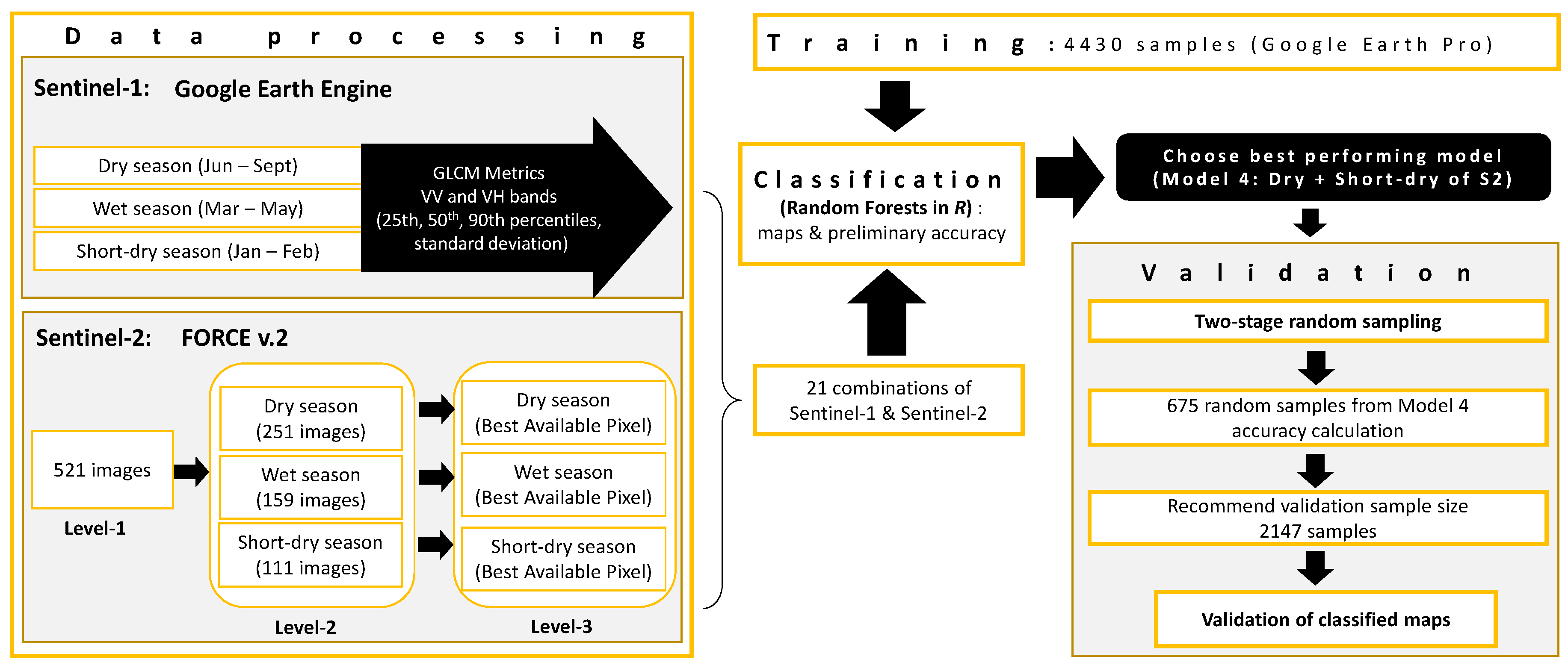
Figure 1. (a) ECMWF (European Center for Medium-Range Weather Forecasts) Re-Analysis (ERA) rainfall average in the study area for 2018/2019, (b) location of the study area in East Africa, (c) Ngorongoro Conservation Area, Tanzania from Google Earth (Digital Globe).
Remotesensing 12 03862 g001
Figure 2. Methodological framework. Google Earth Engine: Gorelick et al. [50]. FORCE (i.e., Framework for Operational Radiometric Correction for Environmental monitoring): Frantz et al. [35].
Remotesensing 12 03862 g002
Figure 3. Output of the best performing model incorporating Sentinel-1 and Sentinel-2 data for both the dry and the short-dry season (i.e., Model 18). Locations AC are the example subsets. that appear in the results.
Remotesensing 12 03862 g003
Figure 4. The overall accuracies and confidence intervals for the 21 model combinations tested. M1 to M7 include Sentinel-2 models; M8 to M14 include Sentinel-1 models and M15 to M21 include Sentinel-1 and -2 models. Coding of model combinations in Table 2.
Remotesensing 12 03862 g004
Figure 5. Producer’s accuracy for different land cover types and models. Coding of model combinations in Table 2.
Remotesensing 12 03862 g005
Figure 6. User’s accuracy for different land cover types and models. Coding of model combinations in Table 2.
Remotesensing 12 03862 g006
Figure 7. Example subsets of the study area: (AC): very-high resolution imagery; (A1C1): land cover maps from Model 18; (A2C2): land cover maps from Model 16; (A3C3): land cover maps from Model 4; (A4C4): land cover maps from Model 8. Coding of model combinations in Table 2.
Remotesensing 12 03862 g007
Figure 8. Overall accuracy results for the 21 models according to sensor and season combinations.
Remotesensing 12 03862 g008
Table 1. Seasonal temporal windows and number of Sentinel images used in each season.
SeasonStart DateTarget DateEnd DateN° of Images
Short-dry1 January 2019 27 January 201928 February 2019111
Wet1 March 201917 April 201931 May 2019159
Dry1 June 201917 September 201930 September 2019251
Table 2. The 21 combinations of the models tested.
SensorData IncludedModel
Sentinel-2 (S2)Dry season S21
Short-dry season S22
Wet season S23
Dry + short-dry seasons S24
Dry + wet seasons S25
Wet + short-dry seasons S26
All seasons S27
Sentinel-1 (S1)Dry season S18
Short-dry season S19
Wet season S110
Dry + short-dry seasons S111
Dry + wet seasons S112
Wet + short-dry seasons S113
All seasons S114
Sentinel-1 and Sentinel-2 combinations (S1 and S2)Dry season S1 and S215
Short-dry seasons S1 and S216
Wet season S1 and S217
Dry + short-dry seasons S1 and S218
Dry + wet seasons S1 and S219
Wet + short-dry seasons S1 and S220
All seasons S1 and S221
Table 3. Confusion matrix for the best performing model incorporating Sentinel-1 and Sentinel-2 data for both the dry and the short-dry season (i.e., Model 18).
ReferenceUser’s Accuracy
BaBuFoGMhShWoTotal
MappedBareland (Ba)73008010820.89
Bushland (Bu)0205229217162710.76
Forest (Fo)07780010860.91
Grassland (G)43012032651912960.93
Montane heath (Mh)01015112560.91
Shrubland (Sh)41031177311450.53
Woodland (Wo)01090221732050.84
Total812181001261561842412141
Producer’s accuracy0.700.920.840.950.840.490.73
Publisher’s Note: MDPI stays neutral with regard to jurisdictional claims in published maps and institutional affiliations.

