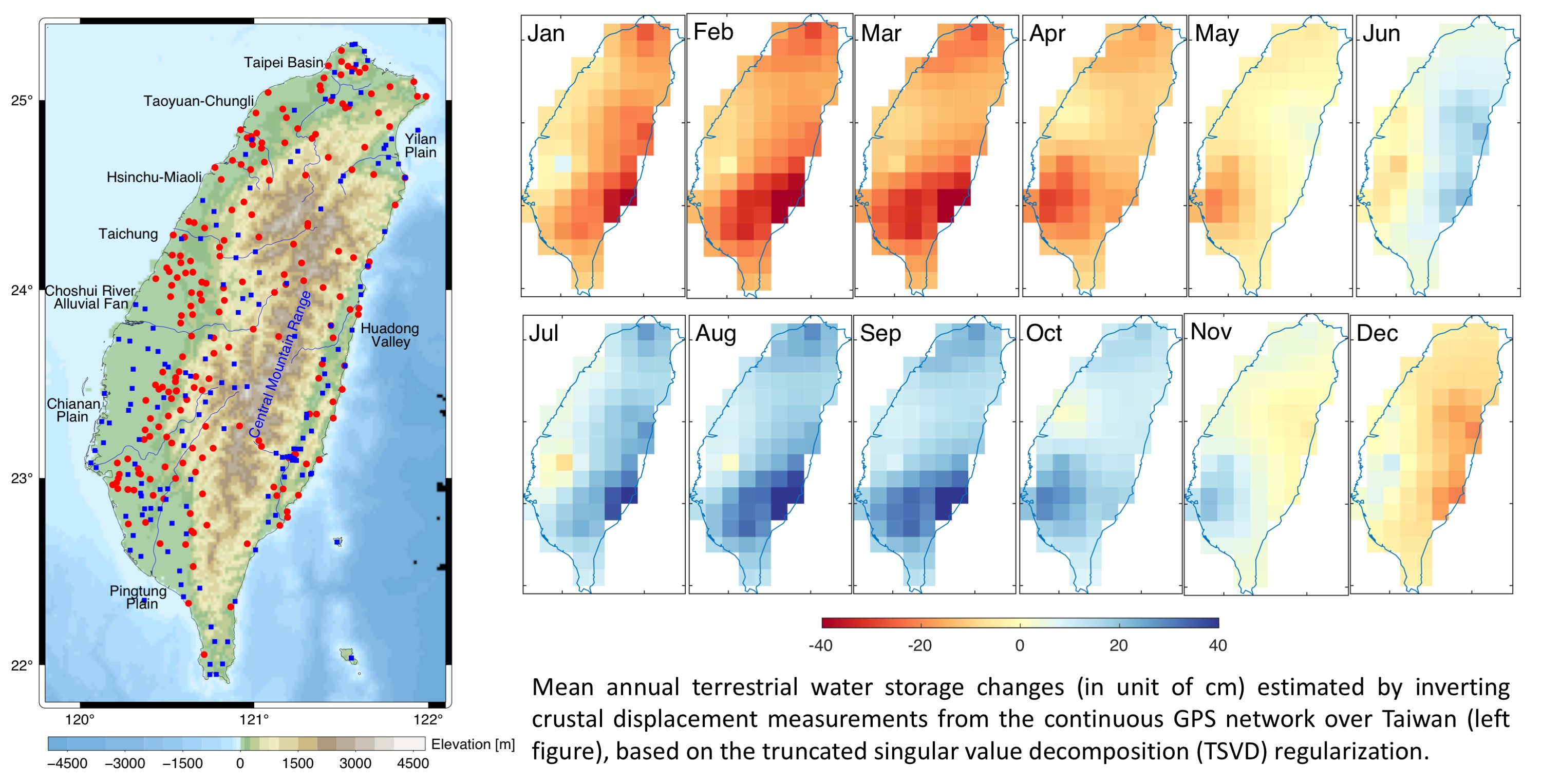
Truncated Singular Value Decomposition Regularization for Estimating Terrestrial Water Storage Changes Using GPS: A Case Study over Taiwan


Abstract

1. Introduction
2. Materials and Methods
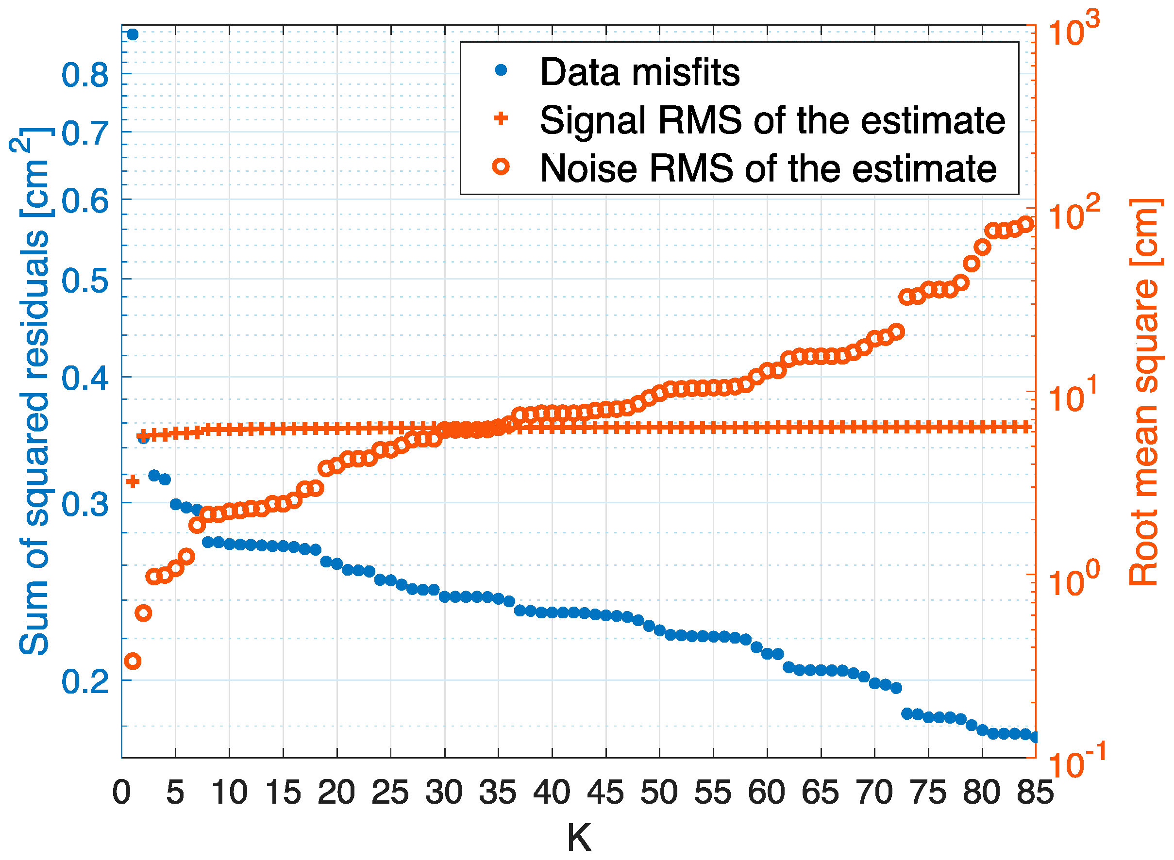
2.1. Truncated Singular Value Decomposition for TWS Estimation
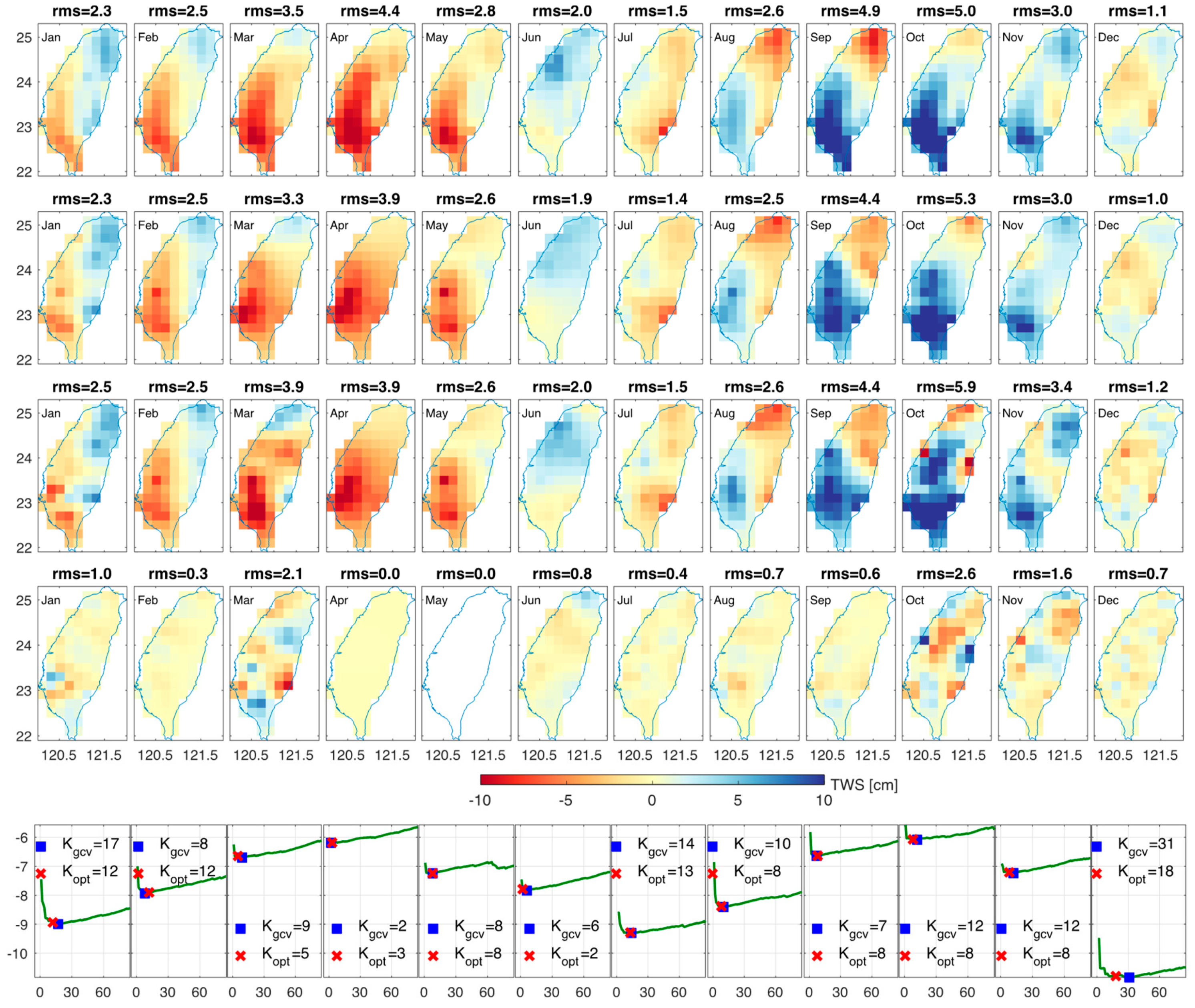
2.2. Generalized Cross Validation for Regularization Parameter Choice
3. Results
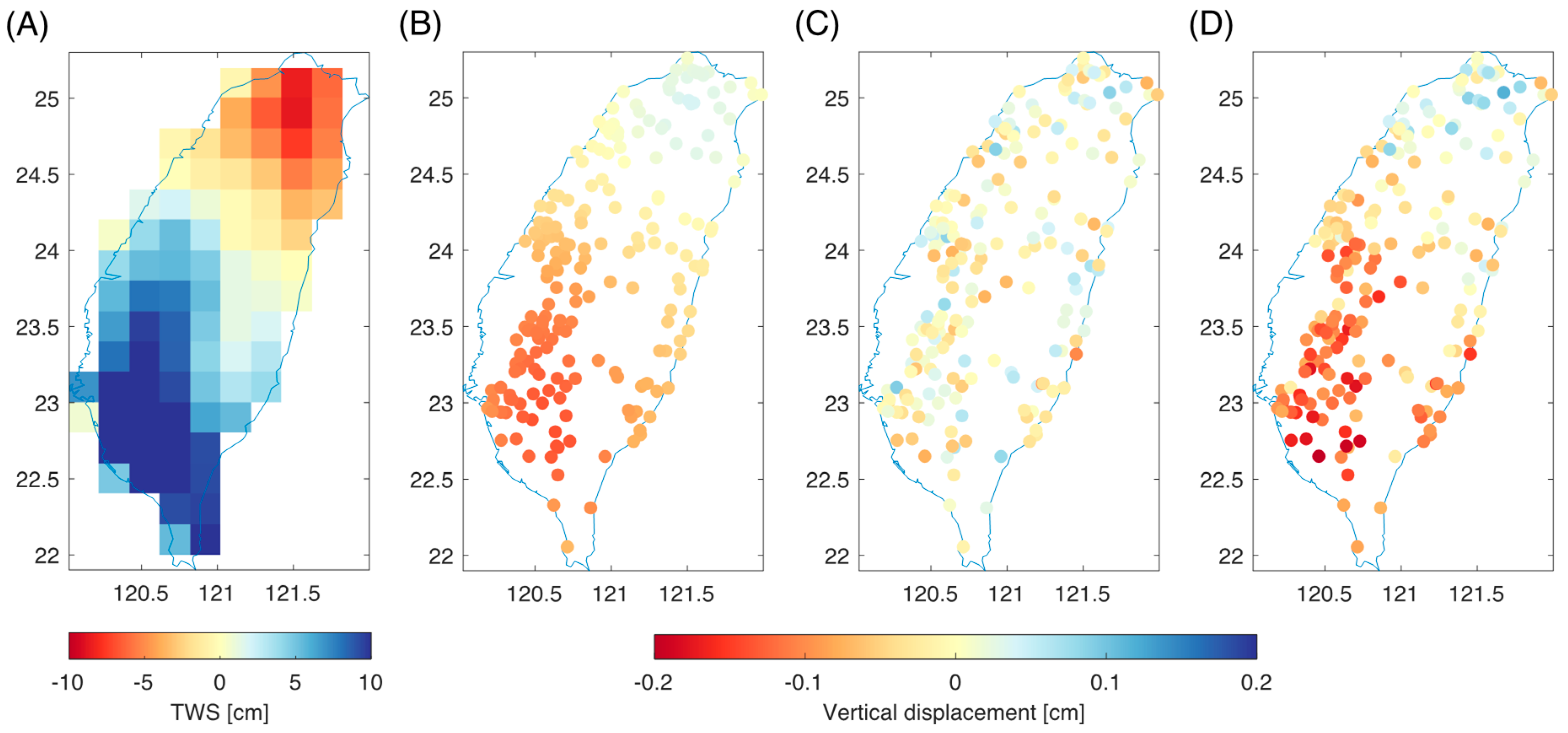
3.1. Simulation
3.2. Real Data Analysis
4. Discussion
5. Conclusions
Author Contributions
Funding
Acknowledgments
Conflicts of Interest
References
- Famiglietti, S. Remote sensing of terrestrial water storage, soil moisture and surface waters. In The State of the Planet: Frontiers and Challenges in Geophysics; American Geophysical Union (AGU): Washington, DC, USA, 2013; pp. 197–207. [Google Scholar]
- Bock, Y.; Melgar, D. Physical applications of GPS geodesy: A review. Rep. Prog. Phys. 2016, 79, 106801. [Google Scholar] [CrossRef] [PubMed]
- Herring, T.A.; Melbourne, T.I.; Murray, M.H.; Floyd, M.; Szeliga, W.M.; King, R.W.; Phillips, D.A.; Puskas, C.; Santillan, M.; Wang, L. Plate Boundary Observatory and related networks: GPS data analysis methods and geodetic products. Rev. Geophys. 2016, 54, 759–808. [Google Scholar] [CrossRef]
- Van Dam, T.; Wahr, J.; Milly, P.C.D.; Shmakin, A.B.; Blewitt, G.; Lavallée, D.; Larson, K.M. Crustal displacements due to continental water loading. Geophys. Res. Lett. 2001, 28, 651–654. [Google Scholar] [CrossRef]
- Bevis, M.; Alsdorf, D.; Kendrick, E.; Fortes, L.P.; Forsberg, B.; Smalley, R.; Becker, J. Seasonal fluctuations in the mass of the Amazon River system and Earth’s elastic response. Geophys. Res. Lett. 2005, 32. [Google Scholar] [CrossRef]
- Tapley, B.D.; Bettadpur, S.V.; Ries, J.; Thompson, P.F.; Watkins, M.M. GRACE Measurements of Mass Variability in the Earth System. Science 2004, 305, 503–505. [Google Scholar] [CrossRef]
- Argus, D.F.; Fu, Y.; Landerer, F.W. Seasonal variation in total water storage in California inferred from GPS observations of vertical land motion. Geophys. Res. Lett. 2014, 41, 1971–1980. [Google Scholar] [CrossRef]
- Borsa, A.A.; Agnew, D.C.; Cayan, D.R. Ongoing drought-induced uplift in the western United States. Science 2014, 345, 1587–1590. [Google Scholar] [CrossRef]
- Argus, D.F.; Landerer, F.W.; Wiese, D.N.; Martens, H.R.; Fu, Y.; Famiglietti, J.S.; Thomas, B.F.; Farr, T.G.; Moore, A.W.; Watkins, M.M. Sustained Water Loss in California’s Mountain Ranges During Severe Drought From 2012 to 2015 Inferred From GPS. J. Geophys. Res. Solid Earth 2017, 122, 10559–10585. [Google Scholar] [CrossRef]
- Fu, Y.; Argus, D.F.; Landerer, F.W. GPS as an independent measurement to estimate terrestrial water storage variations in Washington and Oregon. J. Geophys. Res. Solid Earth 2015, 120, 552–566. [Google Scholar] [CrossRef]
- Adusumilli, S.; Borsa, A.A.; Fish, M.A.; McMillan, H.K.; Silverii, F. A Decade of Water Storage Changes Across the Contiguous United States from GPS and Satellite Gravity. Geophys. Res. Lett. 2019, 46, 13006–13015. [Google Scholar] [CrossRef]
- Fok, H.; Liu, Y. An Improved GPS-Inferred Seasonal Terrestrial Water Storage Using Terrain-Corrected Vertical Crustal Displacements Constrained by GRACE. Remote. Sens. 2019, 11, 1433. [Google Scholar] [CrossRef]
- Liu, Y.; Fok, H.S.; Tenzer, R.; Chen, X. Akaike’s Bayesian Information Criterion for the Joint Inversion of Terrestrial Water Storage Using GPS Vertical Displacements, GRACE and GLDAS in Southwest China. Entropy 2019, 21, 664. [Google Scholar] [CrossRef]
- Zhang, B.; Yao, Y.; Fok, H.; Hu, Y.; Chen, Q. Potential Seasonal Terrestrial Water Storage Monitoring from GPS Vertical Displacements: A Case Study in the Lower Three-Rivers Headwater Region, China. Sensors 2016, 16, 1526. [Google Scholar] [CrossRef] [PubMed]
- Hsu, Y.-J.; Fu, Y.; Bürgmann, R.; Hsu, S.-Y.; Lin, C.-C.; Tang, C.-H.; Wu, Y.-M. Assessing seasonal and interannual water storage variations in Taiwan using geodetic and hydrological data. Earth Planet. Sci. Lett. 2020, 550, 116532. [Google Scholar] [CrossRef]
- Tikhonov, A.N. Solution of Incorrectly Formulated Problems and the Regularization Method. Sov. Math. Dokl. 1963, 4, 1035–1038. [Google Scholar]
- Hansen, P.C.; O’Leary, D.P. The Use of the L-Curve in the Regularization of Discrete Ill-Posed Problems. SIAM J. Sci. Comput. 1993, 14, 1487–1503. [Google Scholar] [CrossRef]
- Hofmann, B. Regularization for Applied Inverse and Ill-Posed Problems: A Numerical Approach; Springer: Leipzig, Germany, 1986. [Google Scholar]
- Golub, G.H.; Van Loan, C.F. Matrix Computations; Johns Hopkins University Press: Baltimore, MD, USA, 2013. [Google Scholar]
- Aster, R.C.; Borchers, B.; Thurber, C.H. Parameter Estimation and Inverse Problems, 3rd ed.; Elsevier: Amsterdam, The Netherlands, 2018. [Google Scholar]
- Rodell, M.; Houser, P.R.; Jambor, U.; Gottschalck, J.; Mitchell, K.; Meng, C.-J.; Arsenault, K.; Cosgrove, B.; Radakovich, J.; Bosilovich, M.; et al. The Global Land Data Assimilation System. Bull. Am. Meteorol. Soc. 2004, 85, 381–394. [Google Scholar] [CrossRef]
- Li, B.; Rodell, M.; Kumar, S.; Beaudoing, H.K.; Getirana, A.; Zaitchik, B.F.; De Goncalves, L.G.; Cossetin, C.; Bhanja, S.; Mukherjee, A.; et al. Global GRACE Data Assimilation for Groundwater and Drought Monitoring: Advances and Challenges. Water Resour. Res. 2019, 55, 7564–7586. [Google Scholar] [CrossRef]
- Becker, J.M.; Bevis, M. Love’s problem. Geophys. J. Int. 2004, 156, 171–178. [Google Scholar] [CrossRef]
- Laske, G.; Masters, G.; Ma, Z.; Pasyanos, M. Update on CRUST1.0—A 1-degree Global Model of Earth’s Crust. Geophys. Res. Abstr. 2013, 15, 2658. [Google Scholar]
- Hansen, P.C. Rank-Deficient and Discrete Ill-Posed Problems; Society for Industrial and Applied Mathematics: Philadelphia, PA, USA, 1998. [Google Scholar]
- Böhm, J.; Niell, A.; Tregoning, P.; Schuh, H. Global Mapping Function (GMF): A new empirical mapping function based on numerical weather model data. Geophys. Res. Lett. 2006, 33. [Google Scholar] [CrossRef]
- Lyard, F.; Lefevre, F.; Letellier, T.; Francis, O. Modelling the global ocean tides: Modern insights from FES2004. Ocean Dyn. 2006, 56, 394–415. [Google Scholar] [CrossRef]
- Altamimi, Z.; Collilieux, X.; Métivier, L. ITRF2008: An improved solution of the international terrestrial reference frame. J. Geod. 2011, 85, 457–473. [Google Scholar] [CrossRef]
- Tregoning, P.; Watson, C.S. Atmospheric effects and spurious signals in GPS analyses. J. Geophys. Res. Space Phys. 2009, 114. [Google Scholar] [CrossRef]
- Fukumori, I. A Partitioned Kalman Filter and Smoother. Mon. Weather. Rev. 2002, 130, 1370–1383. [Google Scholar] [CrossRef]
- Kim, S.-B.; Lee, T.; Fukumori, I. Mechanisms Controlling the Interannual Variation of Mixed Layer Temperature Averaged over the Niño-3 Region. J. Clim. 2007, 20, 3822–3843. [Google Scholar] [CrossRef]
- Tang, C.-H.; Hsu, Y.-J.; Barbot, S.; Moore, J.D.P.; Chang, W.-L. Lower-crustal rheology and thermal gradient in the Taiwan orogenic belt illuminated by the 1999 Chi-Chi earthquake. Sci. Adv. 2019, 5, eaav3287. [Google Scholar] [CrossRef]
- Cheng, F.-Y.; Chen, Y. Variations in soil moisture and their impact on land–air interactions during a 6-month drought period in Taiwan. Geosci. Lett. 2018, 5, 26. [Google Scholar] [CrossRef]
- Hung, C.-W.; Shih, M.-F. Analysis of Severe Droughts in Taiwan and its Related Atmospheric and Oceanic Environments. Atmosphere 2019, 10, 159. [Google Scholar] [CrossRef]
- Hsu, W.-C.; Chang, H.-C.; Chang, K.-T.; Lin, E.-K.; Liu, J.-K.; Liou, Y.-A. Observing Land Subsidence and Revealing the Factors That Influence It Using a Multi-Sensor Approach in Yunlin County, Taiwan. Remote Sens. 2015, 7, 8202–8223. [Google Scholar] [CrossRef]
- Hung, W.-C.; Hwang, C.; Chen, Y.-A.; Zhang, L.; Chen, K.-H.; Wei, S.-H.; Huang, D.-R.; Lin, S.-H. Land Subsidence in Chiayi, Taiwan, from Compaction Well, Leveling and ALOS/PALSAR: Aquaculture-Induced Relative Sea Level Rise. Remote Sens. 2018, 10, 40. [Google Scholar] [CrossRef]
- Chen, C.-S.; Chen, Y.-L. The Rainfall Characteristics of Taiwan. Mon. Weather Rev. 2003, 131, 1323–1341. [Google Scholar] [CrossRef]
- Huang, W.-C.; Chiang, Y.; Wu, R.-Y.; Lee, J.-L.; Lin, S.-H. The Impact of Climate Change on Rainfall Frequency in Taiwan. Terr. Atmos. Ocean. Sci. 2012, 23, 553. [Google Scholar] [CrossRef]
- Kuo, Y.-C.; Lee, M.-A.; Lu, M.-M. Association of Taiwan’s Rainfall Patterns with Large-Scale Oceanic and Atmospheric Phenomena, Advances in Meteorology. 27 December 2015. Available online: https://www.hindawi.com/journals/amete/2016/3102895/ (accessed on 31 August 2020).
- Hung, W.-C.; Hwang, C.; Chang, C.-P.; Yen, J.-Y.; Liu, C.-H.; Yang, W.-H. Monitoring severe aquifer-system compaction and land subsidence in Taiwan using multiple sensors: Yunlin, the southern Choushui River Alluvial Fan. Environ. Earth Sci. 2010, 59, 1535–1548. [Google Scholar] [CrossRef]
- Hwang, C.; Yang, Y.; Kao, R.; Han, J.; Shum, C.K.; Galloway, D.L.; Sneed, M.; Hung, W.-C.; Cheng, Y.-S.; Li, F. Time-varying land subsidence detected by radar altimetry: California, Taiwan and North China. Sci. Rep. 2016, 6, 28160. [Google Scholar] [CrossRef]
- Li, B.; Rodell, M.; Sheffield, J.; Wood, E.; Sutanudjaja, E. Long-term, non-anthropogenic groundwater storage changes simulated by three global-scale hydrological models. Sci. Rep. 2019, 9, 1–13. [Google Scholar] [CrossRef]
- Zhou, Y.; Li, W. A review of regional groundwater flow modeling. Geosci. Front. 2011, 2, 205–214. [Google Scholar] [CrossRef]
- Hsu, L.; Bürgmann, R. Surface creep along the Longitudinal Valley fault, Taiwan from InSAR measurements. Geophys. Res. Lett. 2006, 33. [Google Scholar] [CrossRef]
- Tapley, B.; Watkins, M.M.; Flechtner, F.; Reigber, C.; Bettadpur, S.; Rodell, M.; Sasgen, I.; Famiglietti, J.S.; Landerer, F.W.; Chambers, D.P.; et al. Contributions of GRACE to understanding climate change. Nat. Clim. Chang. 2019, 9, 358–369. [Google Scholar] [CrossRef]
- Wang, L.; Davis, J.L.; Hill, E.M.; Tamisiea, M.E. Stochastic filtering for determining gravity variations for decade-long time series of GRACE gravity. J. Geophys. Res. Solid Earth 2016, 121, 2915–2931. [Google Scholar] [CrossRef]
- Chen, C.-T.; Hu, J.-C.; Lu, C.-Y.; Lee, J.-C.; Chan, Y.-C. Thirty-year land elevation change from subsidence to uplift following the termination of groundwater pumping and its geological implications in the Metropolitan Taipei Basin, Northern Taiwan. Eng. Geol. 2007, 95, 30–47. [Google Scholar] [CrossRef]


Publisher’s Note: MDPI stays neutral with regard to jurisdictional claims in published maps and institutional affiliations. |
© 2020 by the authors. Licensee MDPI, Basel, Switzerland. This article is an open access article distributed under the terms and conditions of the Creative Commons Attribution (CC BY) license (http://creativecommons.org/licenses/by/4.0/).
Share and Cite
Lai, Y.R.; Wang, L.; Bevis, M.; Fok, H.S.; Alanazi, A. Truncated Singular Value Decomposition Regularization for Estimating Terrestrial Water Storage Changes Using GPS: A Case Study over Taiwan. Remote Sens. 2020, 12, 3861. https://doi.org/10.3390/rs12233861
Lai YR, Wang L, Bevis M, Fok HS, Alanazi A. Truncated Singular Value Decomposition Regularization for Estimating Terrestrial Water Storage Changes Using GPS: A Case Study over Taiwan. Remote Sensing. 2020; 12(23):3861. https://doi.org/10.3390/rs12233861
Chicago/Turabian StyleLai, Yen Ru, Lei Wang, Michael Bevis, Hok Sum Fok, and Abdullah Alanazi. 2020. "Truncated Singular Value Decomposition Regularization for Estimating Terrestrial Water Storage Changes Using GPS: A Case Study over Taiwan" Remote Sensing 12, no. 23: 3861. https://doi.org/10.3390/rs12233861
APA StyleLai, Y. R., Wang, L., Bevis, M., Fok, H. S., & Alanazi, A. (2020). Truncated Singular Value Decomposition Regularization for Estimating Terrestrial Water Storage Changes Using GPS: A Case Study over Taiwan. Remote Sensing, 12(23), 3861. https://doi.org/10.3390/rs12233861