Visualizing Near Infrared Hyperspectral Images with Generative Adversarial Networks

Abstract

The visualization of near infrared hyperspectral images is valuable for quick view and information survey, whereas methods using band selection or dimension reduction fail to produce good colors as reasonable as corresponding multispectral images. In this paper, an end-to-end neural network of hyperspectral visualization is proposed, based on the convolutional neural networks, to transform a hyperspectral image of hundreds of near infrared bands to a three-band image. Supervised learning is used to train the network where multispectral images are targeted to reconstruct naturally looking images. Each pair of the training images shares the same geographic location and similar moments. The generative adversarial framework is used with an adversarial network to improve the training of the generating network. In the experimental procedure, the proposed method is tested for the near infrared bands of EO-1 Hyperion images with LandSat-8 images as the benchmark, which is compared with five state-of-the-art visualization algorithms. The experimental results show that the proposed method performs better in producing naturally looking details and colors for near infrared hyperspectral images.

1. Introduction

Hyperspectral satellite images have significant advantages in the recognition of ground contents, but they are not easily understood by the human eye. A hyperspectral image usually has hundreds of 16-bits quantized bands, which is converted to an 8-bits Red-Green-Blue (RGB) image for screen presentation, i.e., hyperspectral visualization. The visualization of hyperspectral images are primarily needed by data centers with preprocessing or distribution systems. For these systems, the visualization produces quick views which help us to judge the availability of selected hyperspectral images. Besides visual recognition, the visualization can improve the accuracy of registration and classification of hyperspectral images because the spatial information is aggregated to present enriched textural and structural characteristics.

Many algorithms have been proposed for hyperspectral visualization, which can be categorized into two groups, namely band-selection-based and dimension-reduction-based. Dimension-reduction-based methods are then classed into linear-projection-based and nonlinear-projection-based to account for the adaptive strategy.

The group of band-selection-based methods choose three separate bands from all the hyperspectral bands. Manually specifying the three bands is experience dependent, therefore is accounted for as an optimization to various purposes such as higher class separability or perceptual color distance. For example, Su et al. [1] used minimum estimated abundance covariance for band selection of true, infrared, and false color composites. Zhu et al. [2] used dominant set extraction to search a graph formulation of band selection which was measured with structure awareness for band informativeness and independence. Amankwah and Aldrich [3] used both mutual information and spatial information to select the bands. Yuan et al. [4] proposed a multitask sparsity pursuit framework with compressive sensing based descriptors and joint sparsity constraint to select the bands. Later on, Yuan et al. [5] proposed a dual clustering method including the contextual information in the clustering process, a new descriptor revealing the image context, and a strategy in selecting the cluster representatives. Demir et al. [6] utilized a one-bit transform to select suitable color bands in low complexity for dedicated hardware implementation.

It is commonly understood that the spectral range of each hyperspectral band is too narrow to hold rich spatial information. Therefore, more bands are involved by means of dimension reduction algorithms. The kind of linear-projection-based methods were first proposed to account for this. For example, Du et al. [7] used principal component analysis (PCA), independent component analysis (ICA), Fisher’s linear discriminant analysis, and their variations for hyperspectral visualization and then compared their performance. Zhu et al. [8] used correlation coefficient and mutual information as the criteria to select three independent components with ICA for color representation. Meka and Chaudhuri [9] visualized hyperspectral images by summing up all the spectral points at each pixel location and optimizing the weights by minimizing the 3-D total-variation norm to improve statistical characteristics of the fused image. Jacobson and Gupta [10] investigated the CIE 1964 tristimulus color matching envelopes and transformed them to the sRGB color space to obtain the fixed linear spectral weighting envelopes. These weights could stretch the visual bands of a hyperspectral image for the linear combination of the red, green, and blue bands, respectively. Algorithms based on PCA or CMF are irrelevant to image content.

In addition to linear projection, the alternative nonlinear methods of dimension reduction were also exploited for hyperspectral visualization. Najim et al. [11] employed the modified stochastic proximity embedding algorithm to cut the spectral dimension as well as to avoid similar colors of dissimilar spectral signatures. Kotwal and Chaudhuri [12] suggested a hierarchical group scheme and bilateral filtering for hyperspectral visualization preserving edges and even the minor details without introducing visible artifacts. In one of the latest work, Kang et al. [13] proposed the decolorization-based hyperspectral image visualization (DHV) framework for hyperspectral visualization. In the DHV framework, hundreds of hyperspectral bands are averaged into nine bands, which are then combined into three bands by means of decolor algorithms [14,15,16,17] for natural images.

The dimension reduction methods assure no natural colors. Therefore, most of them cannot produce good colors except for the work related to color-matching function (CMF) in [10] where CIE 1964 was considered. Motivated by [10], many variations were proposed. Mahmood and Scheunders [18] used the wavelet transform for hyperspectral visualization by fusing CMFs at the low-level subbands and denoising at the high-level subbands. Moan et al. [19] excluded irrelevant bands by comparing entropy between bands, segmented remained bands by thresholding the CMFs, and used the normalized information at second and third orders to select the bands with minimal redundancy and maximal informative content. Sattar et al. [20] used dimension reduction methods, including PCA, maximum noise fraction, and ICA, to get nine bands from a hyperspectral image, and then combined them with the CMF stretching for higher class separability and consistent rendering. Masood et al. [21] proposed spectral residual and phase quaternion Fourier transform to generate the saliency maps in both spatial and spectral domains, which were concatenated with the hyperspectral bands and CMFs to linearly combine the color image.

Although CMF-based linear methods can achieve good color and details, researchers have noticed that better visualization methods should adapt to local characteristics, i.e., using different visualization strategies for different categories of pixels. To illustrate more salient features, Cui et al. [22] clustered the spectral signature of image pixels, mapped the points to the human vision color space, and then performed the convex optimization on cluster representatives and interpolation of the remaining spectral samples. Long et al. [23] introduced the principle of equal variance to divide all hyperspectral bands into three subgroups of uniformly distributed energy, and treated normal pixels and outliers separately using two different mapping methods to enhance global contrast. Cai et al. [24] proposed a feature-driven multilayer visualization technique by analyzing the spatial distribution and importance of each endmember and then visualize it adaptively based on its commonness. Erturk et al. [25] used bilateral filters to extract the base and detail images, reducing contrast in the base image but preserving the detail so that the significance of the detail image can be enhanced, which is a high-dynamic-range (HDR) technique for display devices. Mignotte [26] used the criterion of preserving spectral distance to measure the agreement between the distance of spectrums associated with each pair of pixels and their $L^{\ast }{a}^{\ast }{b}^{\ast }$ (also written as $lab$) perceptual color distance in the final three-band image, which led to the optimization of a nonstationary Markov random field. Liao et al. [27] proposed a fusion approach based on constrained manifold learning, which preserves the image structures by forcing pixels with similar signatures being displayed with similar colors.

Although many algorithms have been proposed, there has been a lack of visualization methods for the near-infrared spectrums. With the increase of hyperspectral sensors, more and more images are captured in the near-infrared band exceeding 760 nm. For example, the spectral range of the shortwave infrared (SWIR) hyperspectral camera mounted on the TIANGONG-1 is 800–2800 nm, and the atmospheric detector mounted on the GAOFEN-5 is also in a similar spectral range. Commonly used algorithms focus on the visualization of images from sensors such as AVIRIS and ROSIS that span to visible light range [28,29,30], which may not be suitable for visualization of the near-infrared detectors.

When the near infrared bands are concerned, it is still challenging to show hyperspectral images with naturally looking colors. Band-selection-based and CMF-based methods may fail because they rely on the visual light bands for natural colors. Dimension reduction tends to produce unnatural colors even for the visual light bands. When the visual light bands are missing, none of the above-mentioned methods can assure the quick view images of natural colors. As an example, our earlier method [31] will lose effect because it requires visual light bands to correct the fused colors.

In this paper, a deep convolutional neural network is designed for the visualization of near infrared hyperspectral bands. It is an end-to-end model, i.e., a hyperspectral image is fed into the network, which outputs a three-band image for visualization. Against the experienced methods for hyperspectral visualization, supervised learning is employed in the newly proposed method to train the network to tune to the expected natural colors. This is accomplished with the repeated observation data. In line with the hyperspectral images, multispectral images covering red, green, and blue spectrums can be easily obtained, which offer the expectations that best describes the terrestrial content of the same place and time. These multispectral images guide the network to fuse natural color and maintain good detail.

The main contributions of this article are listed.

• The visualization of near-infrared hyperspectral images is delicately discussed for the first time in response to the growing trend.
• An end-to-end deep convolution network is designed to visualize hyperspectral images, which is very straightforward and flexible to adapt to a variety of transformation styles.
• A discriminator network is introduced to improve the training quality.

The rest of this article is arranged as follows. In Section 2, the proposed method is presented where the adversarial framework, network architecture, training, and preprocessing are uncovered in detail. In Section 3 and Section 4, the newly proposed method is tested for the EO-1 Hyperion data without visual light bands, which is compared with five state-of-the-art visualization methods to prove its feasibility. In Section 5, the new method is tested for the TIANGONG-1 shortwave infrared bands. Section 6 presents an extended experiment for the visualization of EO-1 Hyperion data where visual light bands are kept. Possible constraints and extensions are discussed in Section 7. Section 8 gives the conclusion.

2. Methodology

The mapping from hyperspectral images to multispectral images may not be a strict dimension reduction process. In our experience, objects should be rendered in fixed colors at a given time. This process implicitly introduces an understanding of the content of the image. We try to describe this mapping process here. The first step is to classify the features, that is, to distinguish small image blocks into different feature categories, such as woodland or artificial buildings. The second step is to find shallow features such as structures and textures. The third step is to color each shallow feature so that it can be understood by the human eye when it is restored back to the image. These mapping steps can be explained with an encoder-decoder system. The first step makes up an encoder for feature extraction, while the second and third steps correspond to a decoder for image reconstruction.

The latest codec methods are implemented using deep convolutional neural networks, which have been widely used for image processing. In image segmentation, features are extracted using deep convolutional networks and aggregated and rendered as labeled images. In conditional image generation, the coded part of the deep convolutional network learns the conditional image features, merges them with the random features, and generates a new image through the decoder. In image restoration, the basic features of defective images are learned by the encoder and then sent to the decoder to repair missing information. These works are essentially the same as the hyperspectral visualization that we understand. Therefore, we will harness an encoder-decoder neural network to visualize the near-infrared hyperspectral images.

2.1. Framework with Neural Networks

The aim of hyperspectral visualization is to fuse a three-band image $I^T$ from a hyperspectral input image $I^H$. For an hyperspectral image, we describe $I^H$ by a real-valued tensor of size $W\times H\times C$ and $I^T$ by $W\times H\times 3$, respectively. Here, W, H, and C denote the width, height, and number of channels, respectively.

Our ultimate goal is to train a generating function G that estimates for a given hyperspectral input image its corresponding three-band multispectral counterpart. To achieve this, a generator network is trained as a feed-forward convolutional neural network (CNN) $G_{{\theta }_G}$ parameterized by ${\theta }_G$. Here ${\theta }_G=\left\{{\omega }_{1:L};B_{1:L}\right\}$ denotes the weights and biases of a L-layer network and is obtained by optimizing a specific loss function $\mathcal{L}\left(·\right)$. For training input images $\left\{I_n^H\right\}$, $n=1,\cdots ,N$ with corresponding output images $\left\{I_n^T\right\}$, $n=1,\cdots ,N$,

$${\widehat{\theta }}_G=arg\underset{{\theta }_G}{min}\frac{1}{N}{\sum }_{n=1}^N\mathcal{L}\left(G_{{\theta }_G}\left(I_n^H\right),I_n^T\right)$$

(1)

is solved, where N denotes the number of training samples. In training, $I^T$ is obtained by finding the multispectral images whose spatial resolution and captured time are similar to $I^H$.

In the remainder of this section, the architecture, loss function, adversarial-based improvement, and data processing of this network will be introduced. For convenience, the proposed method is called Hyperspectral Visualization of Convolutional Neural Networks, or HVCNN for short.

2.2. Generative Network: Architecture

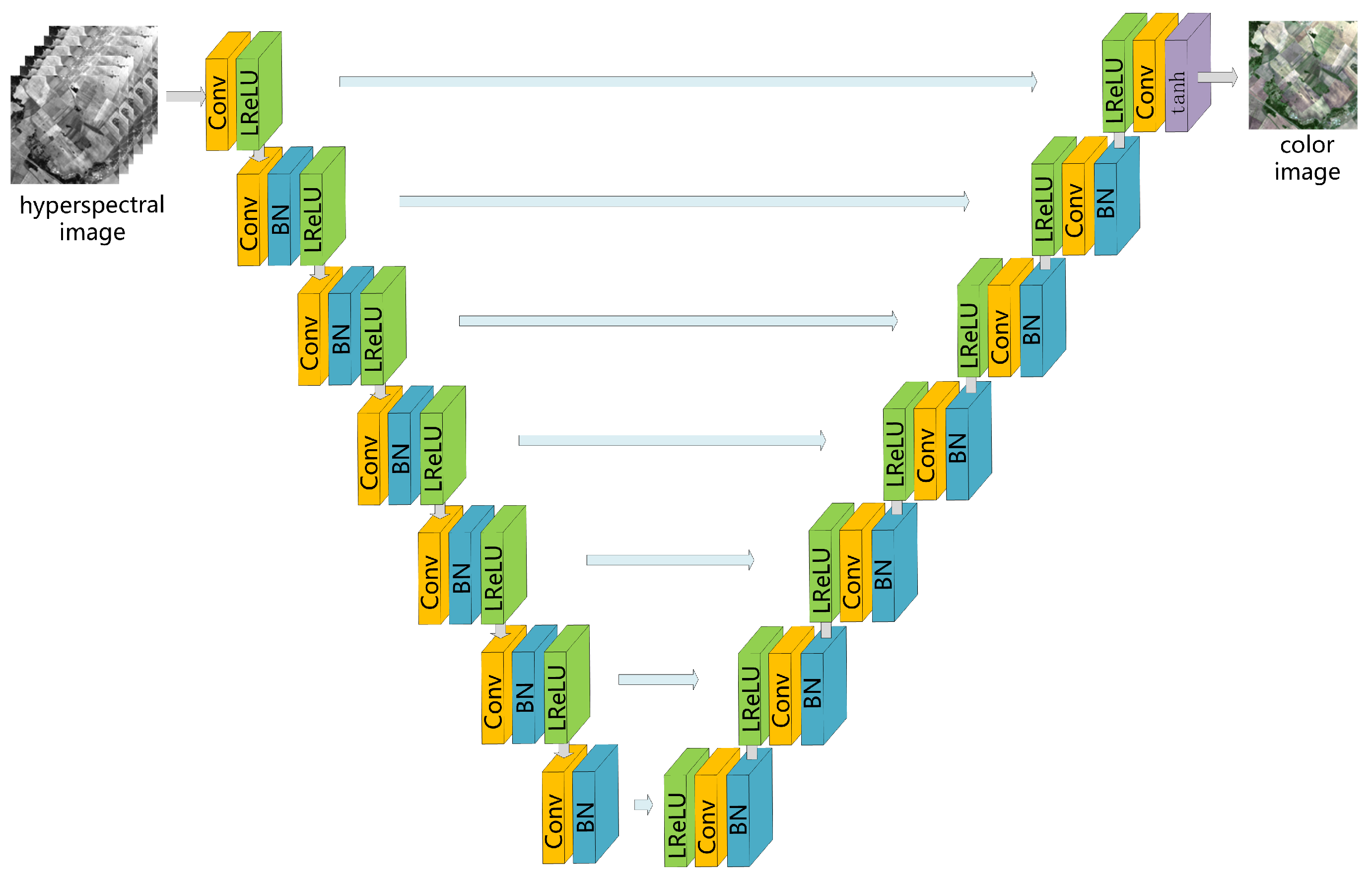
To describe the encoding-decoding process, the U-Net architecture [32,33] is used. The encoder is a downsampled convolutional network to aggregate features, where the stride between adjacent layers is 2. The typical input is a 128 × 128-sized multichannel image, then the encoder network has 7 layers to output a small number of high-level features. The filter sizes are 4 × 4 for all convolutional layers. The possible depth values are 64, 128, 256 as listed in

Table 1. Parameters of the convolutional layers.

Layer ID	Filter Size	Kernel Number	Stride
Encoder
1	4 × 4	64	2
2	4 × 4	128	2
3	4 × 4	256	2
4	4 × 4	512	2
5	4 × 4	512	2
6	4 × 4	512	2
7	4 × 4	512	2
Decoder
1	4 × 4	1024	2
2	4 × 4	1024	2
3	4 × 4	1024	2
4	4 × 4	512	2
5	4 × 4	256	2
6	4 × 4	128	2
7	4 × 4	3	2
Discriminator
1	4 × 4	64	2
2	4 × 4	128	2
3	4 × 4	256	2
4	4 × 4	512	1
5	4 × 4	1	1

. The first convolutional layer is followed by a Leaky-ReLU function for activation, while other convolutional layers are followed by a batch norm (BN) layer and a Leaky-ReLU layer.

Symmetrical to the encoder, the decoder part contains seven 4 × 4 transposed convolutions with a stride of 2. Low-level features have higher resolution to hold position and detail, but they are noisy and of few semantics. On the contrary, high-level features have stronger semantic information, but details are not perceivable. Concatenation is then used to combine low-level features and high-level features to improve model performance. In other words, the input of each transposed convolutional layer in the decoder is a thicker feature formed by concatenating the output of the previous layer and the corresponding encoder layer output. The function tanh is used for activation of the last convolutional layer. Therefore, the entire network has a total of 14 convolutional layers, as is shown in Figure 1.

2.3. Adversarial Network: Architecture and Loss Function

It is commonly known that the performance of a generator can be improved by a discriminator, which leads to a generative adversarial network (GAN). To distinguish the real target image from the generated color image samples, a discriminator network D is further defined with parameter ${\theta }_D$. We adopt the idea in GANs where ${\theta }_D$ is optimized along with G in an alternating manner to solve the minimum-maximum adversarial problem under the expectation $\mathbb{E}$ and distribution p:

$$\begin{array}{c}\hfill \underset{G}{min}\underset{D}{max}\mathbb{E}{}_{I^T\sim p_{train}\left(I^T\right)}\left[log{D}_{{\theta }_D}\left(I^T\left|\right|I^H\right)\right]+\\ \hfill \mathbb{E}{}_{I^H\sim p_G\left(I^H\right)}\left[log\left(1-D_{{\theta }_D}\left(G_{{\theta }_G}\left(I^H\right)\left|\right|I^H\right)\right)\right].\end{array}$$

(2)

Here $\left|\right|$ denotes that two images are combined into one image as the input of the discriminator.

This formula trains a high-quality generative model G to fool the discriminator D as much as possible. The discriminator D is trained to distinguish generated images from real images. Alternate training allows the generator and discriminator to find high-quality solutions in each single-step iteration, and they upgrade as the opponents upgrade. In this way, the generator can learn a solution that is highly similar to the target image.

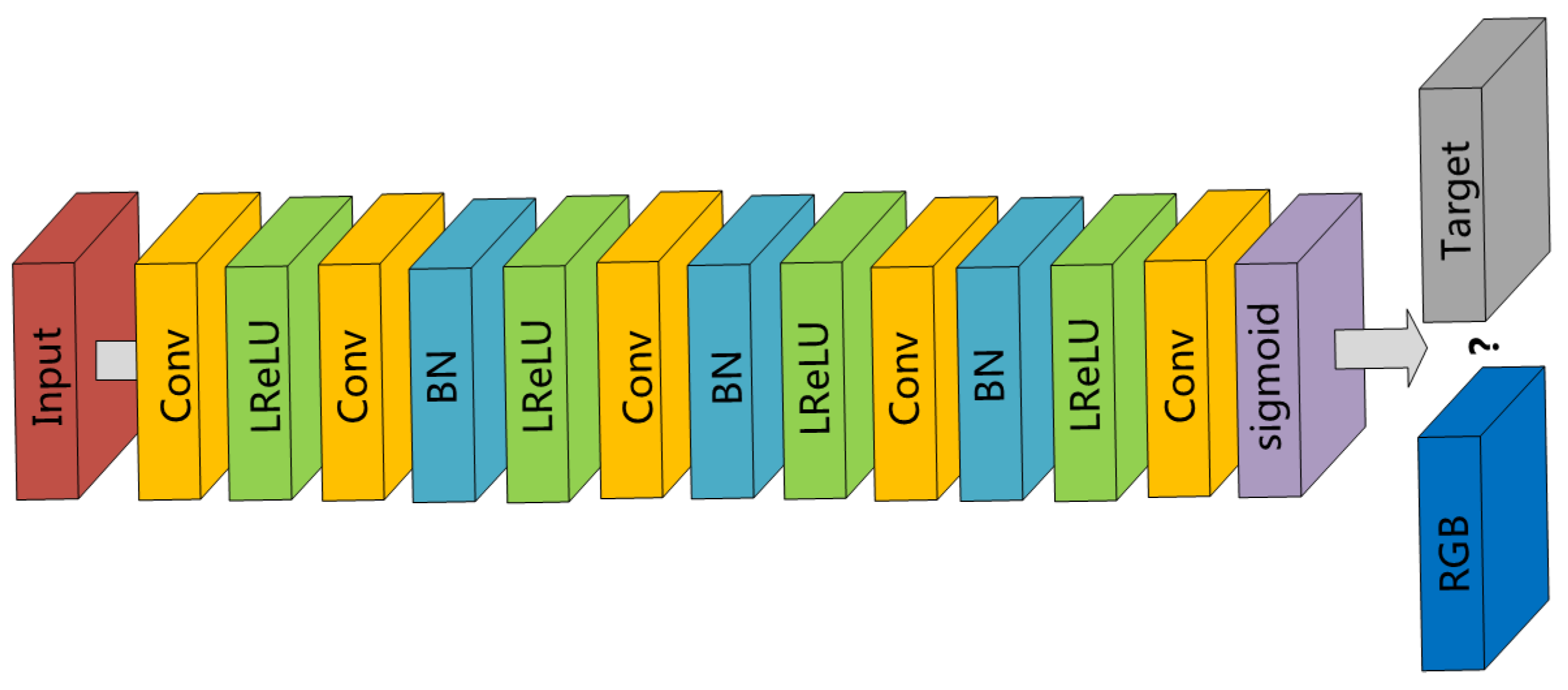
In our method, the adversarial network is built upon CNNs (see Figure 2), too. It contains five convolutional layers. The sigmoid function is used in the last layer as the activation function to assess the probability of the group to which each image belongs.

2.4. Generative Network: Loss Function

The definition of the generative loss function ${\mathcal{L}}_G$ is critical for the performance of the generator network. In our model, the generative loss is formulated as the weighted sum of two components—content loss and adversarial loss for minimization, i.e.,

$${\mathcal{L}}_G=\alpha {\mathcal{L}}_{\mathrm{con}}+{\mathcal{L}}_{\mathrm{adv}}.$$

(3)

The content loss ${\mathcal{L}}_{\mathrm{con}}$ is defined with the ${\ell }_1$ norm, i.e., pixel-wise mean absolute error (MAE). MAE represents the average error margin of the predicted value, regardless of the direction of the error. Compared to the mean square error (MSE) which is easier to be solved, MAE is more robust to outliers. ${\mathcal{L}}_{\mathrm{con}}$ is calculated with

$${\mathcal{L}}_{\mathrm{con}}=\frac{1}{W\times H\times C}\sum _{x=1}^W\sum _{y=1}^H\sum _{z=1}^C\left|I_{x,y,z}^T-G{\left(I^H\right)}_{x,y,z}\right|.$$

(4)

The adversarial loss ${\mathcal{L}}_{\mathrm{adv}}$ is defined based on the probability of the discriminator $D\left(G\left(I^H\right)\right)$ on all training samples as

$${\mathcal{L}}_{\mathrm{adv}}=-\frac{1}{N}{\sum }_{n=1}^{N}log{D}_{{\theta }_D}\left(G_{{\theta }_G}\left(I^H\right)\left|\right|I^H\right),$$

(5)

where $D_{{\theta }_D}\left(G_{{\theta }_G}\left(I^H\right)\left|\right|I^H\right)$ denotes the probability that the reconstructed image $G_{{\theta }_G}\left(I^H\right)$ from the input image $I^H$ is an accepted color image, and N denotes the number of training samples. To better update the gradient, $-log\left(D\left(·\right)\right)$ is minimized instead of $log\left(1-D\left(·\right)\right)$.

2.5. Preprocessing

Prior to the network training, each pair of hyperspectral images and the counterpart three-band image should preferably have the same quantization range to speed up network convergence. This can be achieved by stretching each band independently to 0–255. On the other hand, affected by the imaging environment and atmospheric pollution, there are many abnormal points in remote sensing images, which are often very bright or very dark. The abnormal points in the target image will degrade the training effect. To solve this problem, a nonlinear stretching method is used. After obtaining the cumulative distribution of the image histogram, the darkest 0.1% and brightest 0.1% of the pixel range are eliminated. All the pixels within the statistical threshold range are linearly stretched to 0–255. It is necessarily pointed out that this operation should be performed not on a small image block but on a large image. For example, in our experiments, each nonlinear stretch is performed on a complete image of more than 1,000,000 pixels.

When further used in the network, the input and output images need adjustment once again, i.e., linearly stretched from $[0,255]$ to $[-1,1]$. The network synthesized image is linearly stretched back to 0 to 255 for manifestation. If it is necessary to obtain a 16-bit output image, the original threshold can be used to map pixel values to the approximate range.

3. Experimental Scheme

The EO-1 Hyperion data were tested to illustrate the feasibility of the proposed method. All the visual light bands were removed from the EO-1 Hyperion data to simulate a near-infrared hyperspectral image. The red, green, and blue bands of the LandSat-8 data were used as the target towards natural color. Therefore, there is no overlapping spectrums between input images and output images.

To identify the performance of the proposed visualization method, a variety of state-of-the-art methods were compared, including the classical principal component analysis method [7] (named as PCA), the Bilateral Filtering based method [12] (named as BF), the Dominant Set Extraction based Band Selection [2] (named as DSEBS), and the Decolorization-based Hyperspectral image Visualization (DHV) framework [13]. Two decolorization models, the Extended RGB2Gray Model (ERM) [15] and the Log-Euclidean metric based Decolorization (LED) [16] suggested in [13] along with the DHV framework, were compared and named as DHV-ERM and DHV-LED, respectively.

Parameters of the proposed method were fixed in the experiment. The sizes of input and output image blocks for training were 128 × 128. The Adam optimizer was used where the parameter $\beta$ was 0.5 and the learning rate was 0.0002. The parameter $\alpha$ in the loss function of the generative network was 100. The training was repeated 200 epochs with the batch size set to 1.

In our algorithm, the 0.1% stretch instead of a linear stretch mapped the image nonlinearly to the range [0, 255]. In order to give a fair comparison, the 0.1% stretch was used for all algorithms. In other words, all the hyperspectral images were 0.1% stretched before putting into the algorithms. This benefited all the competing algorithms by increasing their contrast levels.

The quality of synthesized RGB images is assessed with metrics. Structural SIMilarity (SSIM) measures the structural similarity. Correlated coefficient (CC) and peak signal to noise ratio (PSNR) measure the radiometric discrepancy. Spectral angle mapper (SAM) [34], relative dimensionless global error in synthesis (ERGAS) [35], and relative average spectral error (RASE) [36] measure the color consistency. Q4 [37] measures the general similarity. The three-band images from the LandSat-8 red, green, and blue bands are set as the reference. The ideal results are 1 for SSIM, CC, and Q4 while 0 for SAM, ERGAS, and RASE.

4. Experiment for the Hyperion Data

In this section, the EO-1 Hyperion data and LandSat-8 data were used in the experiment for training and evaluation. All the Hyperion and LandSat-8 images were carefully registered. For all the 242 bands of the Hyperion data, 113 spectral bands (42–55, 82–97, 102–119, 134–164, 187–220) were used while others were removed due to uncalibration, noise, or falling into the visual light spectrums (bands 10–41). A total of 4418 pairs of patches were used for training which were extracted from 16 pairs of Hyperion and LandSat-8 images.

The fused images and digital evaluations are presented in this section. Five state-of-the-art methods of hyperspectral visualization are compared to the proposed method. In the experimental procedure, Hyperion images are visualized with geographically matched LandSat-8 images as benchmark for comparison. All the produced images are evaluated to show the ability in preserving details and colors.

4.1. Visual Comparison

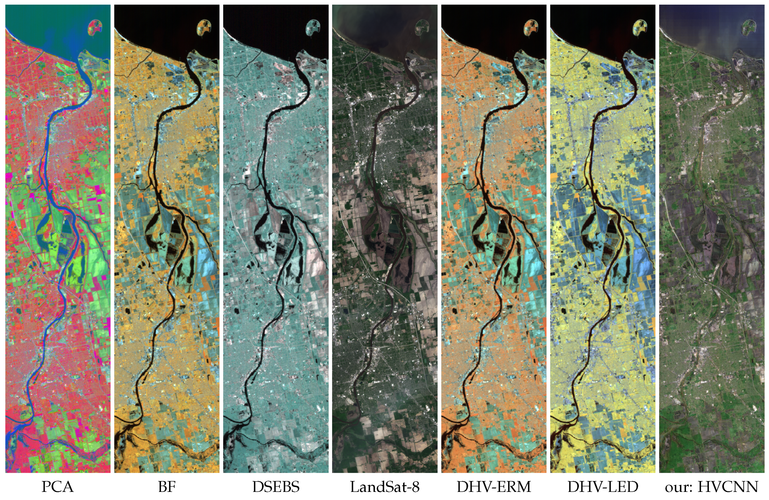
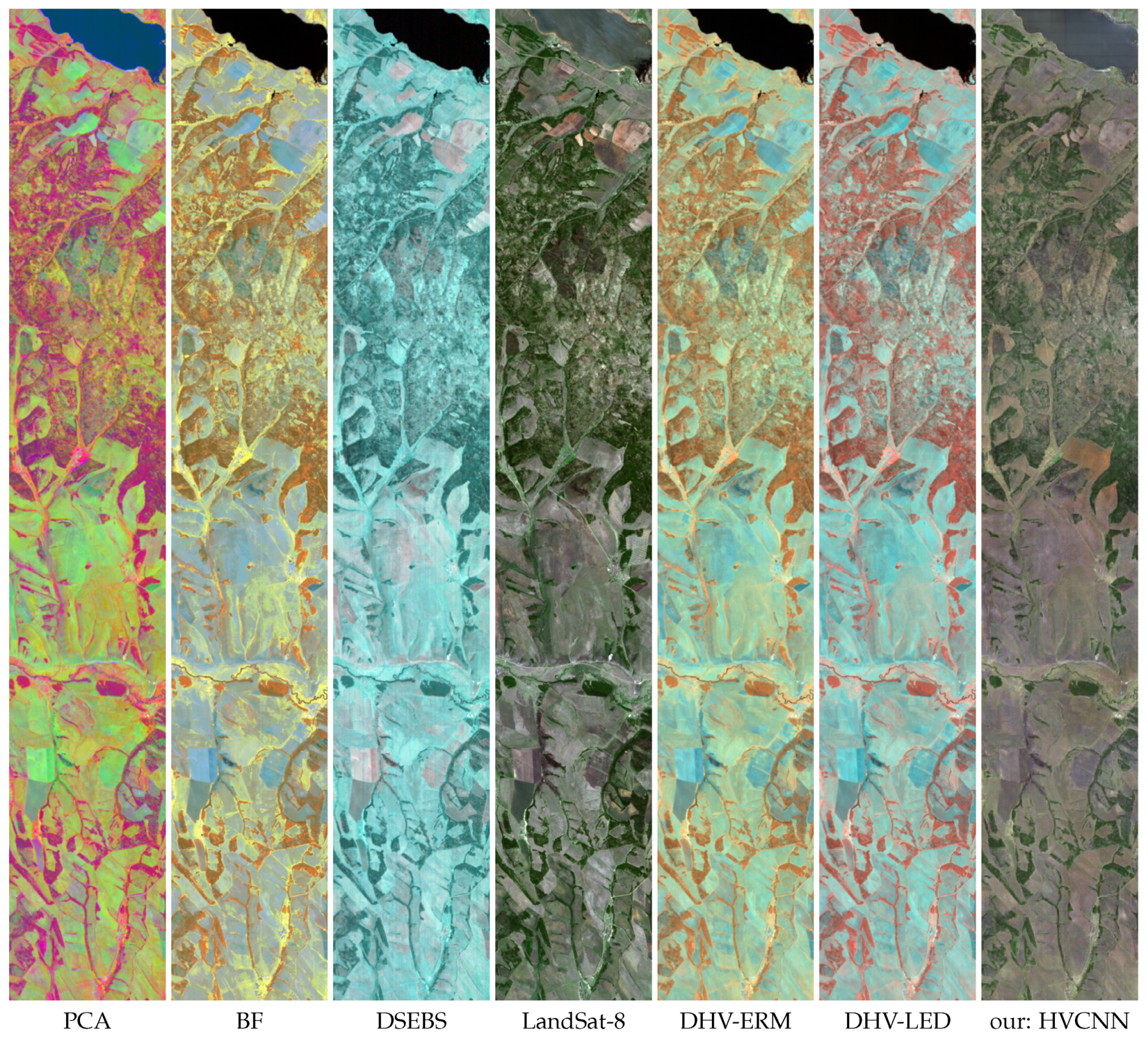
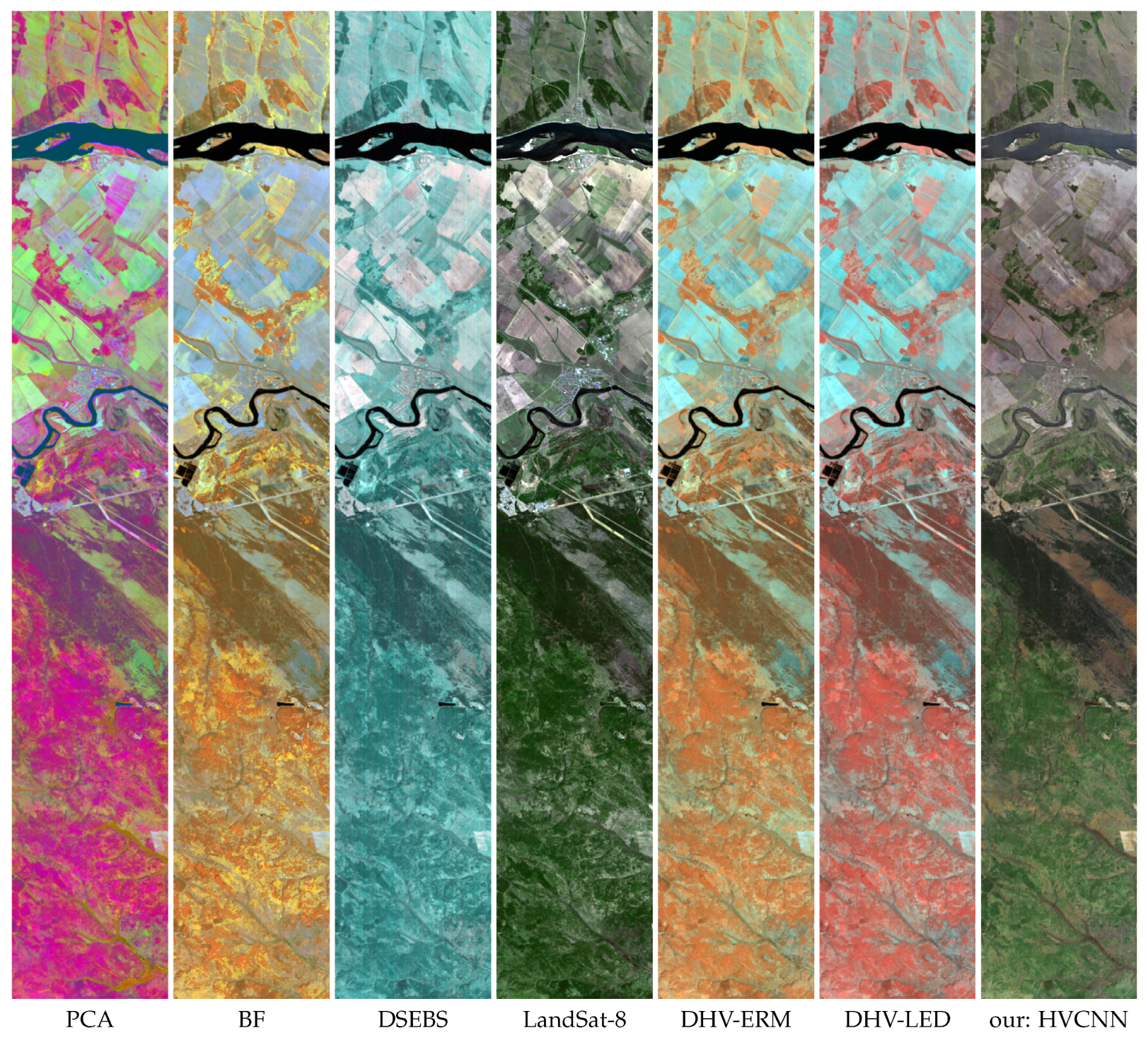
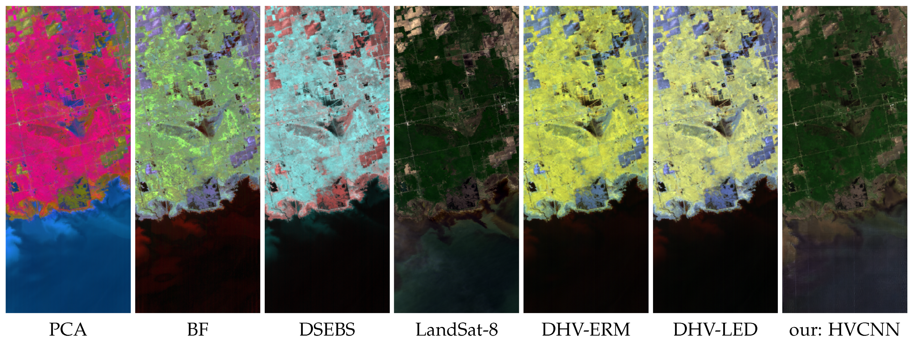
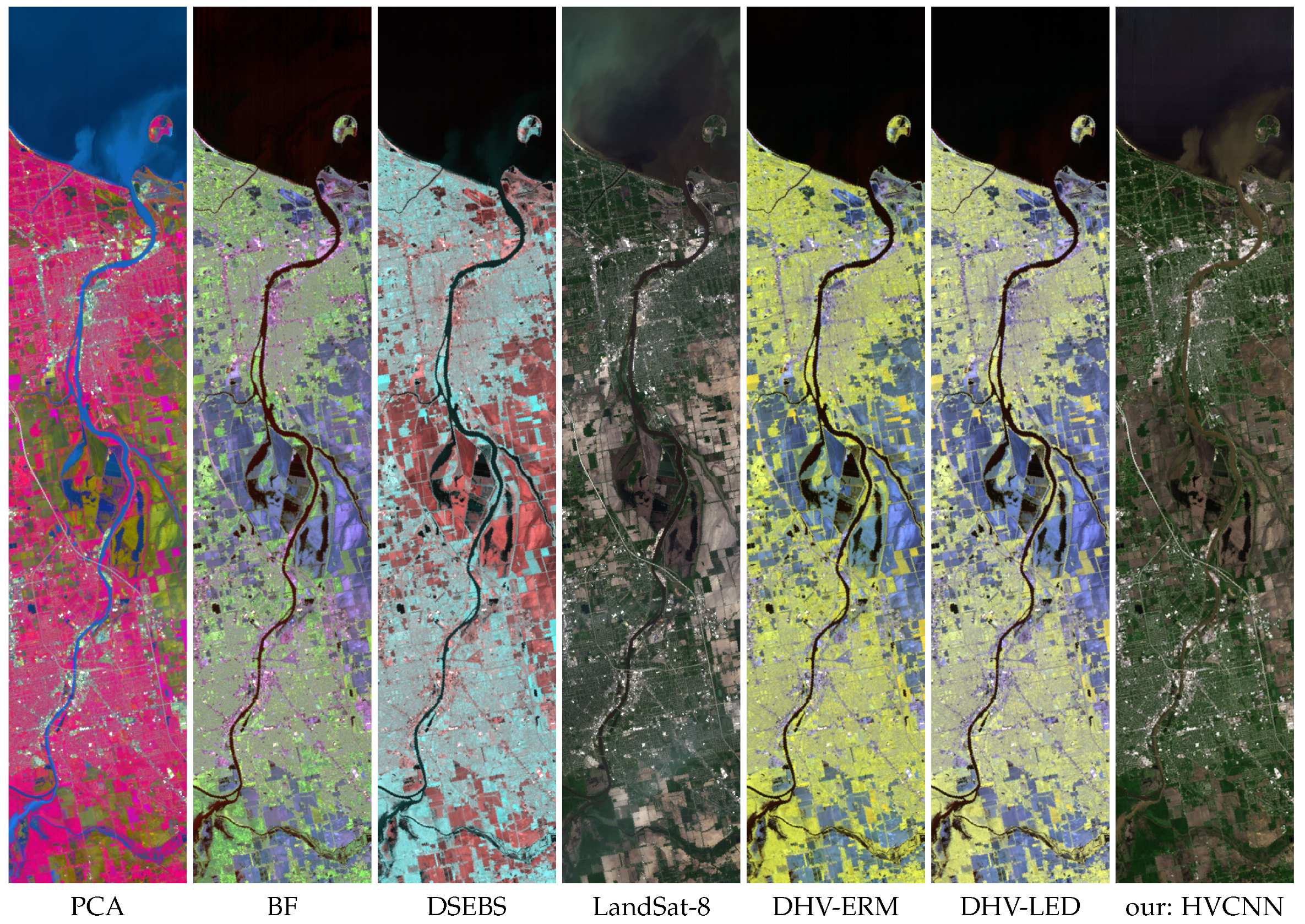
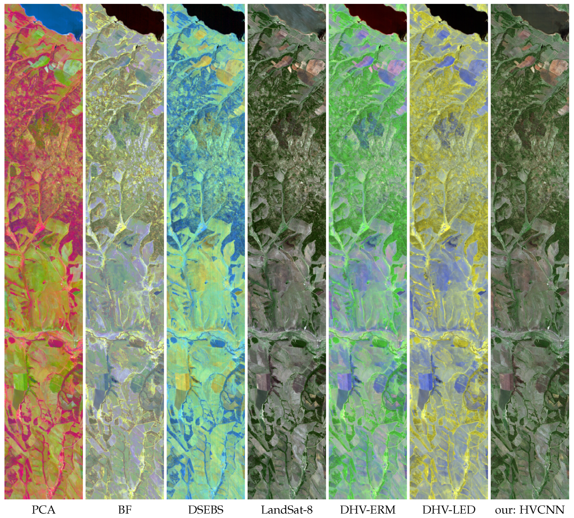
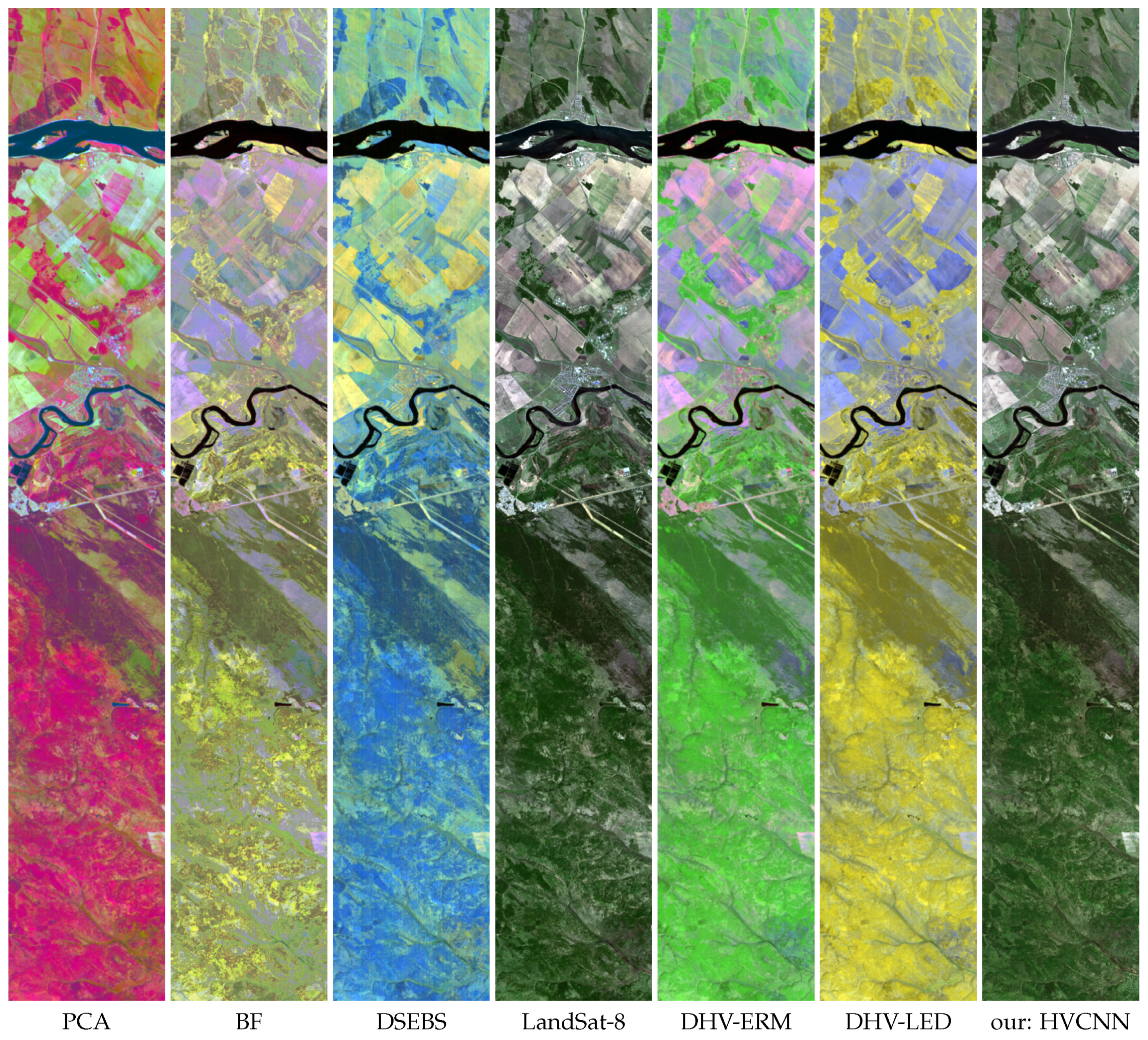
Figure 3, Figure 4, Figure 5 and Figure 6 demonstrate the visualization results of Hyperion images without visual light bands. It is easy to conclude from the comparisons that the colors of the images generated by our method are far more readable than competing methods. For example, the vegetation areas appear green, farmlands and bare lands appear dark gray, and artificial buildings appear light white. These are in line with the visual cognition of the human eye, making it easier to distinguish the categories of ground objects manually.

In addition to visual identification of large objects, natural colors are also helpful for observing structural information in images. In our synthetic result in Figure 4, the staggered concrete pavement, the connected houses, and the surrounding green vegetation constitute a clearly structured city image. For other methods, however, the color difference between the pavement and the surrounding environment is less distinct, which requires careful observation to distinguish the contours.

4.2. Digital Comparison

The SAM, ERGAS, and RASE errors in

Table 2. Evaluation of visualized Hyperion image 1 (visual light bands removed).

	SSIM	CC	PSNR	SAM	ERGAS	RASE	Q4
PCA	0.398	0.359	8.025	0.589	3.102	2.970	0.134
BF	0.239	0.148	8.324	0.378	2.805	2.869	0.133
DSEBS	0.345	0.337	9.553	0.360	2.741	2.491	0.181
DHV-ERM	0.257	0.165	8.148	0.406	2.920	2.928	0.126
DHV-LED	0.184	0.021	6.892	0.311	3.336	3.383	0.099
HVCNN	0.500	0.696	15.975	0.218	1.240	1.189	0.490

,

Table 3. Evaluation of visualized Hyperion image 2 (visual light bands removed).

	SSIM	CC	PSNR	SAM	ERGAS	RASE	Q4
PCA	0.573	0.620	10.561	0.365	1.004	1.004	0.292
BF	0.215	0.435	10.925	0.236	0.949	0.962	0.365
DSEBS	0.445	0.618	12.113	0.132	0.848	0.839	0.522
DHV-ERM	0.263	0.453	10.685	0.236	0.980	0.989	0.365
DHV-LED	0.066	0.281	9.545	0.190	1.114	1.128	0.261
HVCNN	0.550	0.638	18.105	0.086	0.419	0.421	0.582

,

Table 4. Evaluation of visualized Hyperion image 3 (visual light bands removed).

	SSIM	CC	PSNR	SAM	ERGAS	RASE	Q4
PCA	0.664	0.669	11.699	0.319	0.725	0.721	0.490
BF	0.525	0.585	11.050	0.163	0.771	0.776	0.497
DSEBS	0.645	0.702	10.413	0.251	0.874	0.836	0.584
DHV-ERM	0.607	0.596	10.899	0.164	0.788	0.790	0.510
DHV-LED	0.637	0.606	10.911	0.207	0.808	0.789	0.524
HVCNN	0.688	0.831	20.176	0.107	0.281	0.272	0.742

and

Table 5. Evaluation of visualized Hyperion image 4 (visual light bands removed).

	SSIM	CC	PSNR	SAM	ERGAS	RASE	Q4
PCA	0.646	0.887	10.787	0.417	0.926	0.877	0.551
BF	0.509	0.762	11.031	0.251	0.870	0.853	0.643
DSEBS	0.654	0.885	12.282	0.258	0.774	0.738	0.770
DHV-ERM	0.587	0.790	11.054	0.248	0.871	0.851	0.662
DHV-LED	0.617	0.795	11.071	0.283	0.888	0.849	0.662
HVCNN	0.669	0.857	18.687	0.137	0.363	0.353	0.766

show that the proposed HVCNN method produces far better color similar to LandSat-8 in all scenes, which is in line with the conclusion of visual comparison. As far as the image detail is concerned, the SSIM values of our method show steadily higher structural similarity to the reference images. As for the radiometric fidelity, the outstanding PSNR scores of our method show that HVCNN can produce LandSat-8 like images from Hyperion near-infrared bands.

The visualization results of image 1 and image 2 are compared in Table 2 and Table 3, respectively. In these tables, the proposed HVCNN method is far superior to other algorithms in the evaluation of all indicators. Due to the spectral inconsistency between the input image and the output image, neither the dimensionality reduction method nor the band selection method can predict the color of the target image effectively. Among the competing algorithms, DSEBS has the best color consistency, while the two DHV methods have the worst color performance, but none of their colors are easily understandable. In contrast, our method can synthesize roughly acceptable colors as Q4 illustrates. At the same time, PSNR and CC also proved that the data authenticity of the new method is better than other methods. The results of SSIM show that our method has an easily recognizable structure.

Table 4 and Table 5 present the visualization results of image 3 and image 4, respectively, which are quite different from the content of the first two images. In these tables, the scores of all algorithms are improved because the features are simple and free of urban areas. In terms of structural information, the effect of the competing algorithm is very close to that of HVCNN. However, the advantages of this method are still obvious in demonstrating better structure and color.

5. Extended Experiment for the TIANGONG-1 Infrared Data

In this section, two images were also tested from the namely short-wave infrared (SWIR) sensor carried on the TIANGONG-1 satellite. TIANGONG-1 is a manned space platform launched by China in 2011. A TIANGONG-1 SWIR image has 64 available bands that span 1000–2500 nm with the 23 nm spectral resolution. The ground resolution is 20 m, and the swath is 10 km.

To visualize the TIANGONG-1 SWIR data is not a strict hyperspectral visualization issue. After removing the bands of low radiometric quality, only 19 bands were available. However, this data was tested because it falls into the near infrared spectrums. In the experiment, the LandSat-8 images of the similar moments were used again as the target for training. All the TIANGONG-1 and LandSat-8 images were carefully registered and resampled to the uniform ground resolution of 30 m. A total of 1062 pairs of patches from other image pairs were extracted for training.

The synthesized images are presented in Figure 7 and Figure 8, which confirm once again that our method is significantly better than the competing algorithms in producing natural colors. Due to the limited quantity and quality of the training data, the fused details are not as good as Hyperion, then the digital evaluations are not included in this paper. Nevertheless, this test proves the stability of the proposed method in pursuing natural color.

6. Extended Experiment: Visualization of Hyperspectral Images Covering Visual Light Spectrums

The purpose of this article is to design a visualization method for near-infrared hyperspectral images so that they can be visually recognized by the human eye. However, the proposed method should not be limited to near-infrared images. Obviously, the supervised-learning-based neural network can also deal with hyperspectral images containing visible light. On the other hand, the algorithms involved in the comparisons are not specifically designed for near-infrared hyperspectral image visualization. Then the above-mentioned comparisons are not strictly fair. Rationally, we hope to know whether the new method can behave as superior as shown in the earlier experiments for a traditional hyperspectral visualization issue that may cover the visual light spectrums. To explore the answer, an additional experiment on Hyperion was appended in the traditional hyperspectral visualization, i.e., to visualize hyperspectral images owning visual light spectrums.

To illustrate the performance when the spectral range of the hyperspectral sensor completely covers the spectral range of the multispectral sensor for reference, training was repeated when all the data and parameters remain the same except for the input images that extended to the visual light spectrums. For all the 242 bands of the Hyperion data, 145 spectral bands (10–55, 82–97, 102–119, 134–164, 187–220) were used while others were removed due to uncalibration or noise. As correlated coefficients are in line with the PSNR evaluations, mutual information (MI) was calculated to measure the similarity between the overall structures.

The visualization results of the full hyperspectral images are presented in Figure 9, Figure 10, Figure 11 and Figure 12. Given a one-by-one comparison for the HVCNN results in Figure 3, Figure 4, Figure 5 and Figure 6, it is easily concluded that the fidelity of the synthesized red bands are greatly improved, making the overall color closer to the target images. At the same time, the edges and contours are clearer. The urban area in Figure 4 and Figure 10 can explain the conclusion strongly. As for the competing algorithms, the colors are slightly improved and the details are greatly improved, but the images are not directly understood yet.

Where the evaluation values in

Table 6. Evaluation of visualized Hyperion image 1 (all bands involved).

	SSIM	CC	PSNR	SAM	ERGAS	RASE	Q4
PCA	0.550	0.861	9.182	0.662	3.001	2.741	0.096
BF	0.306	0.501	9.878	0.457	2.553	2.530	0.167
DSEBS	0.237	0.582	7.759	0.403	3.415	3.229	0.076
DHV-ERM	0.236	0.486	8.272	0.396	2.967	3.044	0.122
DHV-LED	0.213	0.556	7.623	0.339	3.306	3.280	0.101
HVCNN	0.753	0.766	23.049	0.152	0.567	0.555	0.759

,

Table 7. Evaluation of visualized Hyperion image 2 (all bands involved).

	SSIM	CC	PSNR	SAM	ERGAS	RASE	Q4
PCA	0.705	0.960	11.406	0.439	0.952	0.938	0.307
BF	0.179	0.590	11.887	0.255	0.883	0.888	0.385
DSEBS	0.082	0.652	9.939	0.192	1.119	1.111	0.255
DHV-ERM	0.067	0.631	10.237	0.233	1.057	1.074	0.288
DHV-LED	0.043	0.673	9.659	0.192	1.140	1.147	0.252
HVCNN	0.746	0.870	19.731	0.119	0.362	0.360	0.770

,

Table 8. Evaluation of visualized Hyperion image 3 (all bands involved).

	SSIM	CC	PSNR	SAM	ERGAS	RASE	Q4
PCA	0.799	1.748	12.662	0.390	0.657	0.645	0.507
BF	0.446	0.655	11.673	0.156	0.729	0.723	0.465
DSEBS	0.645	1.138	11.143	0.264	0.792	0.768	0.501
DHV-ERM	0.585	0.850	13.189	0.159	0.598	0.607	0.627
DHV-LED	0.361	0.240	11.448	0.136	0.732	0.742	0.442
HVCNN	0.868	1.800	25.801	0.051	0.146	0.142	0.923

and

Table 9. Evaluation of visualized Hyperion image 4 (all bands involved).

	SSIM	CC	PSNR	SAM	ERGAS	RASE	Q4
PCA	0.767	2.144	11.398	0.460	0.863	0.817	0.615
BF	0.417	0.780	11.528	0.182	0.810	0.805	0.603
DSEBS	0.647	1.606	11.145	0.344	0.902	0.842	0.653
DHV-ERM	0.576	1.068	13.287	0.119	0.617	0.658	0.781
DHV-LED	0.379	0.501	10.493	0.202	0.899	0.907	0.588
HVCNN	0.836	2.058	25.648	0.060	0.162	0.158	0.962

are concerned, both data fidelity and color consistency are improved. For image 3 and 4, the PSNR values have reached 25 dB, and the Q4 values are over 0.9, which show that the HVCNN results could be understood as normal RGB images. Competing algorithms fail to fuse expected colors, but they have good structure and detail according to SSIM and MI.

7. Discussion

7.1. Training Details

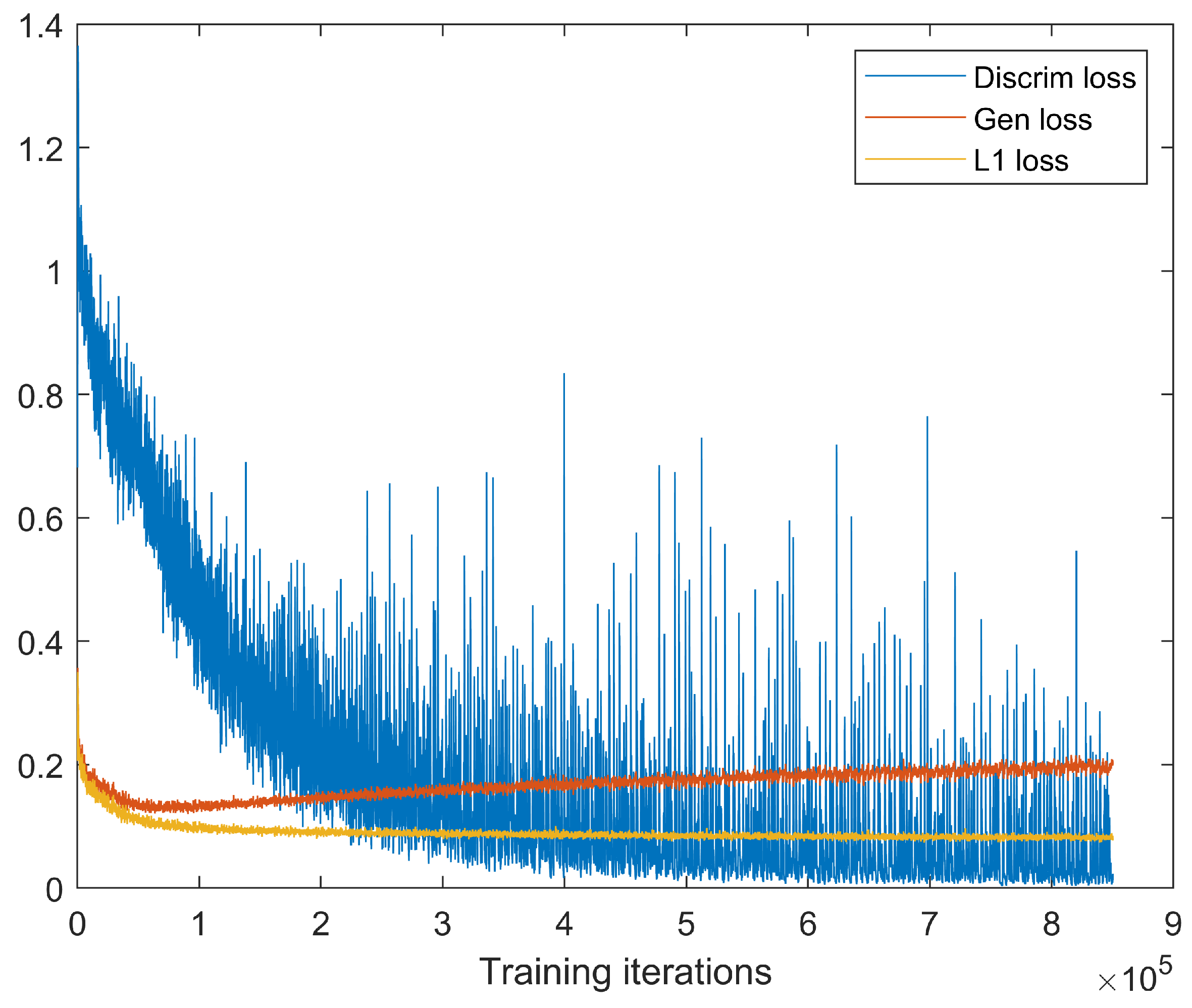
In the training stage, the standard GAN training approach is adopted, i.e., alternatively updating the parameters of the generator and discriminator networks. We expect to produce good details and colors as corresponding multispectral images. Although the ${\ell }_1$ loss does not encourage high-frequency details, in many cases it can capture the low-frequency information accurately. Therefore, in the training process of the generated network, the ${\ell }_1$ loss was endowed with a high weight to enforce the correctness at the low frequencies. This restricts the discriminator to model high-frequency structures.

Figure 13 records the converging trends. As shown in the figure, the ${\ell }_1$ loss decreases rapidly and tends to be stable after 200,000 iterations. Then, with the improvement of the discriminator network, the insufficient high-frequency detail from the generator’s output gradually levels up the loss of the generator network, which pushes the generator to update itself for better performance. Finally, the balance is reached after 700,000 iterations.

7.2. Seasonal Effects

Different color styles result from different seasons and locations. For some locations, our model implicitly learns different color styles from the training image pairs. Then the network can output the appropriate style according to the style of the input data if training images of corresponding moment are provided. This is accomplished when the hyperspectral image and multispectral image of the training data pair are taken from the same moment. In addition, it is also possible to map hyperspectral images of different seasons to the same season. This can be achieved by fixing the capturing time of multispectral images in all training data pairs. The latter facilitates comparisons to quickly discover new information in the ground. However, no matter which scheme is adopted, a large amount of training data is required. The feasibility of our method has been proven for limited data, and its feasibility for large-scale data can be expected. However, a lot of work is needed to fully prove this by data collection and experiment, which can be expected in the future work.

7.3. Effects of Nonlinear Stretching

Although both the hyperspectral data and the introduced multispectral image are 16-bit quantization, they have to be stretched to the range 0–255 for displaying in screens. There are two stretching strategies: stretching to 0 to 255 after synthesis or stretching before synthesis. These two methods are equal if the upper and lower boundaries used for stretching are unchanged. However, for neural networks, stretching in advance is more preferable because different ranges of input and output may increase the difficulty of training the network.

Furthermore, 0.1% is suggested in our method for the nonlinear threshold. It is small enough to keep up high data fidelity. On the contrary, a larger ratio will bring higher contrast and clearer details, which is conducive to human observation. In this case, however, the data authenticity has a large loss. For instance, the 2% stretch causes about 4% of RMSE loss for LandSat-8 images, which may impact quantitative applications.

8. Conclusions

In this paper, the visualization of near infrared images is addressed for the first time. The solution to this issue is described as a decoder-encoder process, modeled with an end-to-end architecture based on convolutional neural networks, and trained with referenced images to obtain naturally looking images. Multispectral images give the expected structures and colors for supervised learning.

The proposed method is compared with five state-of-the-art algorithms to validate the performance. The EO-1 Hyperion images are used for testing without the visual light bands. The comparison results show that the proposed method can produce LandSat-8 like images for the visual-light-free Hyperion images, which yields the best color fidelity, as well as the structural information most similar to that of the contemporary multispectral images.

The versatility of the new method is also tested for more scenes. The extended experiment on TIANGONG-1 shortwave infrared restates the advantage of our method in producing natural colors even with limited data. The supplementary experiment on Hyperion images of full spectrums shows that the proposed method can also be used for the traditional hyperspectral visualization issue.

References

1. Su, H.; Du, Q.; Du, P. Hyperspectral Image Visualization Using Band Selection. IEEE J. Sel. Top. Appl. Earth Obs. Remote Sens. 2014, 7, 2647–2658. [Google Scholar] [CrossRef]
2. Zhu, G.; Huang, Y.; Lei, J.; Bi, Z.; Xu, F. Unsupervised Hyperspectral Band Selection by Dominant Set Extraction. IEEE Trans. Geosci. Remote Sens. 2016, 54, 227–239. [Google Scholar] [CrossRef]
3. Amankwah, A.; Aldrich, C. A spatial information measure method for hyperspectral image visualization. In Proceedings of the 2015 IEEE International Geoscience and Remote Sensing Symposium (IGARSS), Milan, Italy, 26–31 July 2015; pp. 4542–4545. [Google Scholar]
4. Yuan, Y.; Zhu, G.; Wang, Q. Hyperspectral Band Selection by Multitask Sparsity Pursuit. IEEE Trans. Geosci. Remote Sens. 2015, 53, 631–644. [Google Scholar] [CrossRef]
5. Yuan, Y.; Lin, J.; Wang, Q. Dual-Clustering-Based Hyperspectral Band Selection by Contextual Analysis. IEEE Trans. Geosci. Remote Sens. 2016, 54, 1431–1445. [Google Scholar] [CrossRef]
6. Demir, B.; Celebi, A.; Erturk, S. A Low-Complexity Approach for the Color Display of Hyperspectral Remote-Sensing Images Using One-Bit-Transform-Based Band Selection. IEEE Trans. Geosci. Remote Sens. 2009, 47, 97–105. [Google Scholar] [CrossRef]
7. Du, Q.; Raksuntorn, N.; Cai, S.S.; Moorhead, R.J. Color display for hyperspectral imagery. IEEE Trans. Geosci. Remote Sens. 2008, 46, 1858–1866. [Google Scholar] [CrossRef]
8. Zhu, Y.; Varshney, P.K.; Chen, H. ICA-based fusion for colour display of hyperspectral images. Int. J. Remote Sens. 2011, 32, 2427–2450. [Google Scholar] [CrossRef]
9. Meka, A.; Chaudhuri, S. A Technique for Simultaneous Visualization and Segmentation of Hyperspectral Data. IEEE Trans. Geosci. Remote Sens. 2015, 53, 1707–1717. [Google Scholar] [CrossRef]
10. Jacobson, N.P.; Gupta, M.R. Design goals and solutions for display of hyperspectral images. IEEE Trans. Geosci. Remote Sens. 2005, 43, 2684–2692. [Google Scholar] [CrossRef]
11. Najim, S.A.; Lim, I.S.; Wittek, P.; Jones, M.W. FSPE: Visualization of Hyperspectral Imagery Using Faithful Stochastic Proximity Embedding. IEEE Geosci. Remote Sens. Lett. 2015, 12, 18–22. [Google Scholar] [CrossRef] [Green Version]
12. Kotwal, K.; Chaudhuri, S. Visualization of Hyperspectral Images Using Bilateral Filtering. IEEE Trans. Geosci. Remote Sens. 2010, 48, 2308–2316. [Google Scholar] [CrossRef] [Green Version]
13. Kang, X.; Duan, P.; Li, S.; Benediktsson, J.A. Decolorization-Based Hyperspectral Image Visualization. IEEE Trans. Geosci. Remote Sens. 2018, 56, 4346–4360. [Google Scholar] [CrossRef]
14. Liu, Q.; Liu, P.X.; Xie, W.; Wang, Y.; Liang, D. GcsDecolor: Gradient Correlation Similarity for Efficient Contrast Preserving Decolorization. IEEE Trans. Image Process. 2015, 24, 2889–2904. [Google Scholar]
15. Liu, Q.; Xiong, J.; Zhu, L.; Zhang, M.; Wang, Y. Extended RGB2Gray conversion model for efficient contrast preserving decolorization. Multimed. Tools Appl. 2017, 76, 14055–14074. [Google Scholar] [CrossRef]
16. Liu, Q.; Shao, G.; Wang, Y.; Gao, J.; Leung, H. Log-Euclidean Metrics for Contrast Preserving Decolorization. IEEE Trans. Image Process. 2017, 26, 5772–5783. [Google Scholar] [CrossRef] [PubMed]
17. Liu, Q.; Leung, H. Variable augmented neural network for decolorization and multi-exposure fusion. Inf. Fusion 2019, 46, 114–127. [Google Scholar] [CrossRef]
18. Mahmood, Z.; Scheunders, P. Enhanced Visualization of Hyperspectral Images. IEEE Geosci. Remote Sens. Lett. 2011, 8, 869–873. [Google Scholar] [CrossRef]
19. Moan, S.L.; Mansouri, A.; Voisin, Y.; Hardeberg, J.Y. A Constrained Band Selection Method Based on Information Measures for Spectral Image Color Visualization. IEEE Trans. Geosci. Remote Sens. 2011, 49, 5104–5115. [Google Scholar] [CrossRef] [Green Version]
20. Sattar, S.; Khan, H.A.; Khurshid, K. Optimized class-separability in hyperspectral images. In Proceedings of the 2016 IEEE International Geoscience and Remote Sensing Symposium (IGARSS), Beijing, China, 10–15 July 2016; pp. 2711–2714. [Google Scholar]
21. Masood, F.; Qazi, I.U.H.; Khurshid, K. Saliency-based visualization of hyperspectral satellite images using hierarchical fusion. J. Appl. Remote Sens. 2018, 12, 046011. [Google Scholar] [CrossRef]
22. Cui, M.; Razdan, A.; Hu, J.; Wonka, P. Interactive Hyperspectral Image Visualization Using Convex Optimization. IEEE Trans. Geosci. Remote Sens. 2009, 47, 1673–1684. [Google Scholar]
23. Long, Y.; Li, H.C.; Celik, T.; Longbotham, N.; Emery, W.J. Pairwise-Distance-Analysis-Driven Dimensionality Reduction Model with Double Mappings for Hyperspectral Image Visualization. Remote Sens. 2015, 7, 7785–7808. [Google Scholar] [CrossRef] [Green Version]
24. Cai, S.; Du, Q.; Moorhead, R.J. Feature-Driven Multilayer Visualization for Remotely Sensed Hyperspectral Imagery. IEEE Trans. Geosci. Remote Sens. 2010, 48, 3471–3481. [Google Scholar] [CrossRef]
25. Erturk, S.; Suer, S.; Koc, H. A High-Dynamic-Range-Based Approach for the Display of Hyperspectral Images. IEEE Geosci. Remote Sens. Lett. 2014, 11, 2001–2004. [Google Scholar] [CrossRef]
26. Mignotte, M. A Multiresolution Markovian Fusion Model for the Color Visualization of Hyperspectral Images. IEEE Trans. Geosci. Remote Sens. 2010, 48, 4236–4247. [Google Scholar] [CrossRef]
27. Liao, D.; Qian, Y.; Zhou, J.; Tang, Y.Y. A Manifold Alignment Approach for Hyperspectral Image Visualization With Natural Color. IEEE Trans. Geosci. Remote Sens. 2016, 54, 3151–3162. [Google Scholar] [CrossRef] [Green Version]
28. Jiang, H.; Lu, N.; Yao, L. A High-Fidelity Haze Removal Method Based on HOT for Visible Remote Sensing Images. Remote Sens. 2016, 8, 844. [Google Scholar] [CrossRef] [Green Version]
29. Jiang, H.; Lu, N. Multi-Scale Residual Convolutional Neural Network for Haze Removal of Remote Sensing Images. Remote Sens. 2018, 10, 945. [Google Scholar] [CrossRef] [Green Version]
30. Ngo, D.; Lee, S.; Kang, B. Robust Single-Image Haze Removal Using Optimal Transmission Map and Adaptive Atmospheric Light. Remote Sens. 2020, 12, 2233. [Google Scholar] [CrossRef]
31. Tang, R.; Liu, H.; Wei, J.; Tang, W. Supervised learning with convolutional neural networks for hyperspectral visualization. Remote Sens. Lett. 2020, 11, 363–372. [Google Scholar] [CrossRef]
32. Ronneberger, O.; Fischer, P.; Brox, T. U-Net: Convolutional Networks for Biomedical Image Segmentation. In Medical Image Computing and Computer-Assisted Intervention, Pt Iii; Lecture Notes in Computer Science; Springer: Cham, Switzerland, 2015; Volume 9351, pp. 234–241. [Google Scholar]
33. Isola, P.; Zhu, J.; Zhou, T.; Efros, A.A. Image-to-Image Translation with Conditional Adversarial Networks. In Proceedings of the 2017 IEEE Conference on Computer Vision and Pattern Recognition (CVPR), Honolulu, HI, USA, 21–26 July 2017; pp. 5967–5976. [Google Scholar]
34. Jagalingam, P.; Hegde, A.V. A Review of Quality Metrics for Fused Image. Aquat. Procedia 2015, 4, 133–142. [Google Scholar] [CrossRef]
35. Du, Q.; Younan, N.H.; King, R.; Shah, V.P. On the Performance Evaluation of Pan-Sharpening Techniques. IEEE Geosci. Remote Sens. Lett. 2007, 4, 518–522. [Google Scholar] [CrossRef]
36. Ranchin, T.; Wald, L. Fusion of high spatial and spectral resolution images: The ARSIS concept and its implementation. Photogramm. Eng. Remote Sens. 2000, 66, 49–61. [Google Scholar]
37. Alparone, L.; Baronti, S.; Garzelli, A.; Nencini, F. A Global Quality Measurement of Pan-Sharpened Multispectral Imagery. IEEE Geosci. Remote Sens. Lett. 2004, 1, 313–317. [Google Scholar] [CrossRef]
Figure 1. Architecture of the generative network for hyperspectral visualization. The left part is an encoder network, and the right part is a decoder network. The input of each transposed convolutional layer in the decoder is a thicker feature formed by concatenating the output of the previous layer and the corresponding encoder layer output.
Remotesensing 12 03848 g001
Figure 2. Architecture of the discriminator.
Remotesensing 12 03848 g002
Figure 3. Visualization results of Hyperion image 1 (113 bands from 773nm to 2355nm by removing the visual light bands).
Remotesensing 12 03848 g003
Figure 4. Visualization results of Hyperion image 2 (113 bands from 773nm to 2355nm by removing the visual light bands).
Remotesensing 12 03848 g004
Figure 5. Visualization results of Hyperion image 3 (113 bands from 773nm to 2355nm by removing the visual light bands).
Remotesensing 12 03848 g005
Figure 6. Visualization results of Hyperion image 4 (113 bands from 773nm to 2355nm by removing the visual light bands).
Remotesensing 12 03848 g006
Figure 7. Visualization results of TIANGONG-1 image 1 (19 bands between 1000 nm and 2500 nm).
Remotesensing 12 03848 g007
Figure 8. Visualization results of the TIANGONG-1 image 2 (19 bands between 1000 nm and 2500 nm).
Remotesensing 12 03848 g008
Figure 9. Visualization results of Hyperion image 1 (145 bands from 457 nm to 2355 nm).
Remotesensing 12 03848 g009
Figure 10. Visualization results of Hyperion image 2 (145 bands from 457 nm to 2355 nm).
Remotesensing 12 03848 g010
Figure 11. Visualization results of Hyperion image 3 (145 bands from 457 nm to 2355 nm).
Remotesensing 12 03848 g011
Figure 12. Visualization results of Hyperion image 4 (145 bands from 457 nm to 2355 nm).
Remotesensing 12 03848 g012
Figure 13. The loss curves in the training procedure.
Remotesensing 12 03848 g013