Article

Robust Data Fusion of UAV Navigation Measurements with Application to the Landing System

Institute for Information Transmission Problems RAS, Bolshoy Karetny per. 19, Build.1, 127051 Moscow, Russia
*
Author to whom correspondence should be addressed.
These authors contributed equally to this work.
Remote Sens. 2020, 12(23), 3849; https://doi.org/10.3390/rs12233849
Submission received: 10 October 2020 / Revised: 11 November 2020 / Accepted: 19 November 2020 / Published: 24 November 2020

Abstract

:
To perform precise approach and landing concerning an aircraft in automatic mode, local airfield-based landing systems are used. For joint processing of measurements of the onboard inertial navigation systems (INS), altimeters and local landing systems, the Kalman filter is usually used. The application of the quadratic criterion in the Kalman filter entails the well-known problem of high sensitivity of the estimate to anomalous measurement errors. During the automatic approach phase, abnormal navigation errors can lead to disaster, so the data fusion algorithm must automatically identify and isolate abnormal measurements. This paper presents a recurrent filtering algorithm that is resistant to anomalous errors in measurements and considers its application in the data fusion problem for landing system measurements with onboard sensor measurements—INS and altimeters. The robustness of the estimate is achieved through the combined use of the least modulus method and the Kalman filter. To detect and isolate failures the chi-square criterion is used. It makes possible the customization of the algorithm in accordance with the requirements for false alarm probability and the alarm missing probability. Testing results of the robust filtering algorithm are given both for synthesized data and for real measurements.

Graphical Abstract

1. Introduction

The integration of data from various sensors is fundamental in the navigation of unmanned aerial vehicles. The use of different physical principle based sensors provides a comprehensive observation of remote objects, but leads to the necessity of mutual calibration of these sensors to obtain homogeneous information in the same units. Sometimes it needs to change the detector or use other sophisticated observation control methods [1]. The data fusion is necessary in remote sensisng when the images of the terrain surface preliminary obtained from satellite are used with current observation from on-board camera [2,3,4,5]. In recent years the use of machine learning methods has become traditional and these methods show good performance in 3 D analysis and reconstruction of the earth surface [6,7]. These methods are applicable to UAV navigation in unknown environment [8,9,10]. However, they are hardly applicable in the navigation and control of objects with continuous and noisy dynamics. This is true especially in conditions of incomplete information and counteraction, when control actions and coordinate estimates must be generated very quickly, because there is practically no time for training and it is impossible to create enough representative training sequence. Here it is necessary to use traditional and reliable methods of the stochastic and adaptive control theory. One should note that these methods contain the stochastic optimization methods in hidden form; therefore, it seems pointless to oppose the machine learning approaches to direct optimization methods. The only advantage of machine learning methods is, most likely, very low requirements for understanding the properties of an optimized system, provided that there is a sufficiently representative training sequence and there is no time limit. For machine learning there is not necessary to have more or less exact mathematical model, but in control of real dynamical systems such model usually exists. As well exists the noise model and it is unreasonable to neglect these models. Different sensors have different noise levels and failure rates or loss of sensitivity, so some of them can serve as indicators of malfunction of others. In this article we use an algorithmic approach to identify such outliers, which allows us to move from traditional Kalman filtering to estimates based on minimizing L 1 errors in error rates and vice versa. This ensures that the assessment procedures are robust in the presence of heavy-tailed accidental outliers. This modification of the estimation procedures makes it possible to use them not only for navigation, but also in solving various problems arising in remote sensing of the earth surface by variuos UAVs observation systems. One shoud stress the impostance of data fusion for autonomous UAV flight and navigation. There is diffrent approaches to this issue such as federative or centered methods of the data fusion [11,12]. There are diffrent approaches to this issue such as federative or centered methods of the data fusion. The federation scheme is very often used in practice, but it does not take into account the possible correlation between parameter under estimation, and for correction of long-term U -type errors it needs to develop a special methodology. It is interesting to use the particle filter to combat anomalies like in [13]. The application of this algorithm in redundant systems also requires additional research. Therefore, in our approach we decided to develop our own algorithm. And in order to avoid the exponential growth of the complexity of the algorithm with an increase in the number of estimated parameters, we tried to develop an algorithm without using the Monte Carlo method. In the work [14] authors use a federated scheme + sigma-point filter (UKF) and the globally optimal estimate is constructed from the estimates of the local filters. They apply the chi-square test, but they control only the covariance matrix of the state vector. Article [14] is aimed at solving the problem of adaptive filtering, but the robustness to anomalous errors in measurements has not been studied.
Abnormal navigation errors during the approach phase can lead to catastrophic consequences. Therefore, increased requirements for accuracy and reliability are necessary to impose on navigation support. High-precision inertial navigation systems (INS) are installed on board of medium and heavy class aircrafts. The availability of measurements of such systems is superior to other types of navigation sensors, which allows to use the INS as the core of integrated navigation systems [15]. A feature of inertial systems is the slow accumulation of errors over time, which must be compensated by other types of navigation sensors. Today the simplest correction method is to use GNSS receivers [16,17]. However, GNSS signals have low noise immunity, which can lead to unavailability of a navigation solution. In this case the automatic landing is provided by airfield-based means: radar systems [18,19] or laser systems [20]. There are also more autonomous solutions based on machine vision methods which do not require the installation of radio equipment on the airfield [3,21]. Abstracting from the specific type of system, one can consider them as sources of measurements in a spherical coordinate system. In the vertical navigation channel on board of the aircraft radio altimeters and air pressure sensors are used. They are usually backed up two or three times.
The problem of joint processing of measurements from various types of navigation sensors is called the data fusion. When the linear model of the system is adequate, data fusion problem is solved by the Kalman filter [15,22,23]. In the processing task of landing systems measurements one has to deal with nonlinear measurements. Working with nonlinear systems we can use the advanced Kalman filter [16,24]. In some cases, when the system has strong nonlinearities, other nonlinear filters are used such as UKF and Sigma-point Kalman Filter [24,25]. Another approach to nonlinear measurements processing is the pseudo-measurement method [26]. The pseudo-measurement method was used in this work, since it showed a sufficiently high efficiency and it is easy to implement (see Section 4.2).
In the indicated modifications of the Kalman filter, a quadratic criterion of optimality is used. It entails high sensitivity of the estimate to anomalous errors in measurements [27,28]. In cases where the covariance of the anomalous measurements is known, the method proposed in [29] can be used. However, in reality there are a lot of cases when the dispersion of anomalous measurements is not known or not determined at all [30]. For the mathematical description of such errors the heavy-tailed distributions are used instead of the Gaussian distribution [31]. The filtering problem for heavy-tailed distributions can be solved approximately using the so-called particle filters, which are based on the Monte Carlo method [13,32]. However, the complexity of such algorithms increases exponentially with the increase of the state space dimension, which requires large computational resources.
In work [33] a robust form of the Kalman filter is proposed, where the M estimate is used:
x ^ ( t i ) = arg min x x ˜ x P 2 + i = 1 N ρ ( H ( i , : ) x y ( i ) ) , ρ ( ϵ ) = ϵ 2 / 2 , if | ϵ | λ , λ | ϵ | 0.5 λ 2 , if | ϵ | > λ .
where x ˜ is prior state vector, P is covariance matrix of the prior state vector, H is observation matrix, y is measurements vector, x A = x A 1 x T . This approach does not require a significant increase in computing resources, and the use of L 1 -norm in the loss function significantly increases the resistance of the estimate to anomalous measurements. Robust properties of estimate based on minimization of L 1 -norm of errors been investigated in [27,28,34]. However, this approach has its drawback. If for some reason an anomalous error has been accumulated in the state estimate, then the estimate will converge to the true values for a long time. This effect is demonstrated in the Figure 1 (graph «Sqr+Huber»), where the response of the estimate to a step input signal is shown.
In works [35,36] to obtain a robust estimate the use of Huber’s M estimate was proposed [27]:
x ^ ( t i ) = arg min x i = 1 M ρ ( L ( i , : ) ( x ˜ x ) ) + i = 1 M ρ ( H ( i , : ) x y ( i ) ) ,
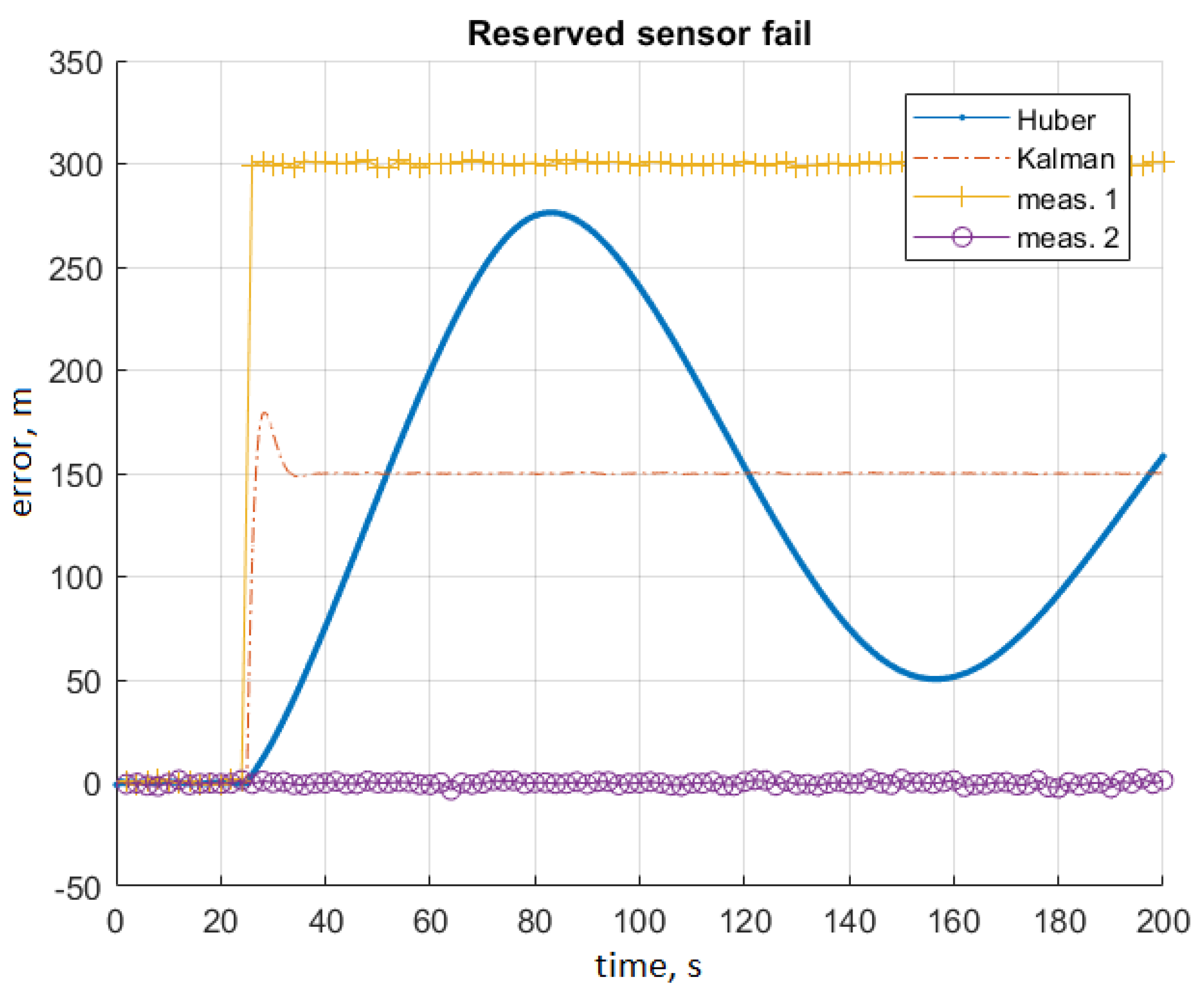
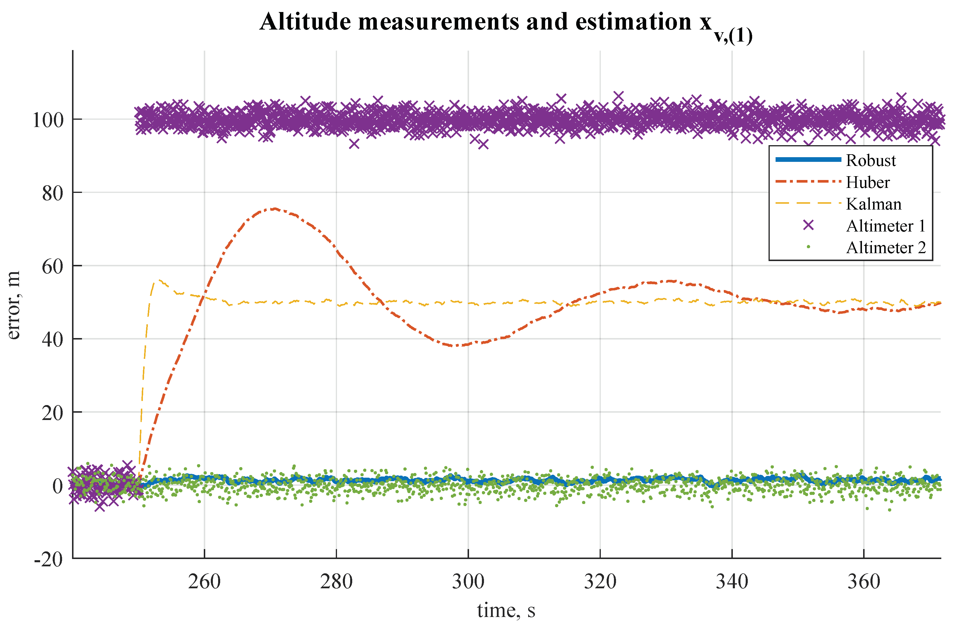
where L L T = P is the Cholesky decomposition for the covariance matrix of the prior state vector. Such estimate made it possible to introduce elements of adaptability into the filter simultaneously with the measurement weights, the weight of the prediction state is calculated. However, this approach does not always lead to the desired results. The transient process can have a sawtooth shape, and the overshoot is comparable to the optimal filter, as shown in the Figure 1 (graph «Huber»). Such behavior of the estimation is unacceptable in the problem of trajectory filtering based on measurements of radar systems, because in measurements there can be jump-like transitions from the antenna side lobe to the main one. Considering the specifics of the problem, the desired filter should be insensitive to short-term surges in measurements and a fast transient, as shown in the Figure 1. Moreover, the estimate (2) cannot be used in systems with redundant measurements. To demonstrate this disadvantage, a numerical simulation was carried out. In this case measurements from two sources of measurements of the same type were processed. On the Figure 2 estimate (2) and measurements from two sensors are shown. It is clear that the filtering error increases with time, although only one dimension contains anomalous measurement errors.
The proposed algorithm also uses robust state estimation. To calculate it an accurate and efficient L 1 -optimization method is used [37]. However, this estimate is not used directly as the output of the filter. Depending on the residuals of the measurements, the covariance matrices of the measurements and the apriori state are calculated, which are then come to the input of the extended Kalman filter. This approach gives great freedom in choosing the weight function for abnormal measurements, which allows to achieve the desired type of transient. The developed algorithm also takes into account that aviation equipment uses redundant navigation sensors to improve navigation reliability. The developed integration algorithm performs automatic detection and isolation of redundant sensor failures based on the chi-square criterion. That is the main scientific contribution of our work.
Section 2 provides a mathematical formulation of the problem. Section 3 provides a general description of the algorithm. Section 4 describes the developed algorithm, its implementation for solving the integration problem is presented in Section 5. Test results are presented in Section 6.

2. Problem Statement

The mathematical task is to estimate the current navigation parameters based on the entire set of available measurements. In other words, it is necessary to obtain an estimate of the current coordinates of the aircraft in real time based on a sample of measurements of the growing volume, that is, to solve the filtering problem. At the time t i , i N , there is a sample of observations Y i = y ( t 0 ) , , y ( t i ) , each observation is a realization of a random variable with a conditional density p y ( y ( t i ) x ( t i ) , Y i 1 ) , where x ( t i ) X , and X is the system state space. When solving the filtering problem, the main interest is the posterior distribution density p ^ x ( x ( t i ) Y i ) . The dynamics of the system can be represented as a Markov process, in which the state of the system x ( t i ) at time t i related to the state of the system x ( t i 1 ) at time t i 1 through the conditional distribution density p x ( x ( t i ) x ( t i 1 ) ) .
It is known that when observations and dynamics of a system are described by linear equations, and p y and p x have Gaussian distributions, the sought density p ^ x ( x ( t i ) Y i ) is also Gaussian and the problem has an analytical solution known as the Kalman filter. In this case, the equations of dynamics and observations have the form:
x ( t i ) = F ( t i 1 , t i ) x ( t i 1 ) + n ( t i 1 , t i ) , y ( t i ) = H ( t i ) x ( t i ) + ξ ( t i ) ,
where F ( t i 1 , t i ) is state prediction matrix; H ( t i ) is observation matrix; n ( t i ) and ξ ( t i ) is vectors of normally distributed random variables such as
E n ( t i 1 , t i ) n T ( t i 1 , t i ) = Q ( t i 1 , t i ) , E ξ ( t i ) ξ ( t i ) = R ( t i ) .
Posterior density distribution parameters p ( x ( t ) Y t ) is a vector of mathematical expectations and covariance matrix are calculated in accordance with the recurrent Kalman algorithm, consistingt of two steps:
  • Prediction:
    x ˜ ( t i ) = F ( t i 1 , t i ) x ^ ( t i 1 ) ,
    P ˜ ( t i ) = F ( t i 1 , t i ) P ^ ( t i 1 ) F T ( t i 1 , t i ) + Q ( t i 1 , t i ) ;
  • Correction of the state estimate based on current measurements:
    d z ( t i ) = y ( t i ) H ( t i ) x ˜ ( t i ) ,
    K = P ˜ ( t i ) H T ( t i ) ( H ( t i ) P ˜ ( t i ) H T ( t i ) + R ( t i ) ) 1 , x ^ ( t i ) = x ˜ ( t i ) + K d z ( t i ) , P ^ ( t i ) = ( I K H ( t i ) ) P ˜ ( t i ) .
Such estimate is optimal according to the criterion of the minimum variance of the estimation error [38,39]. The Kalman filter allows all available measurement information to be taken into account for state estimation.

3. Robust Filter

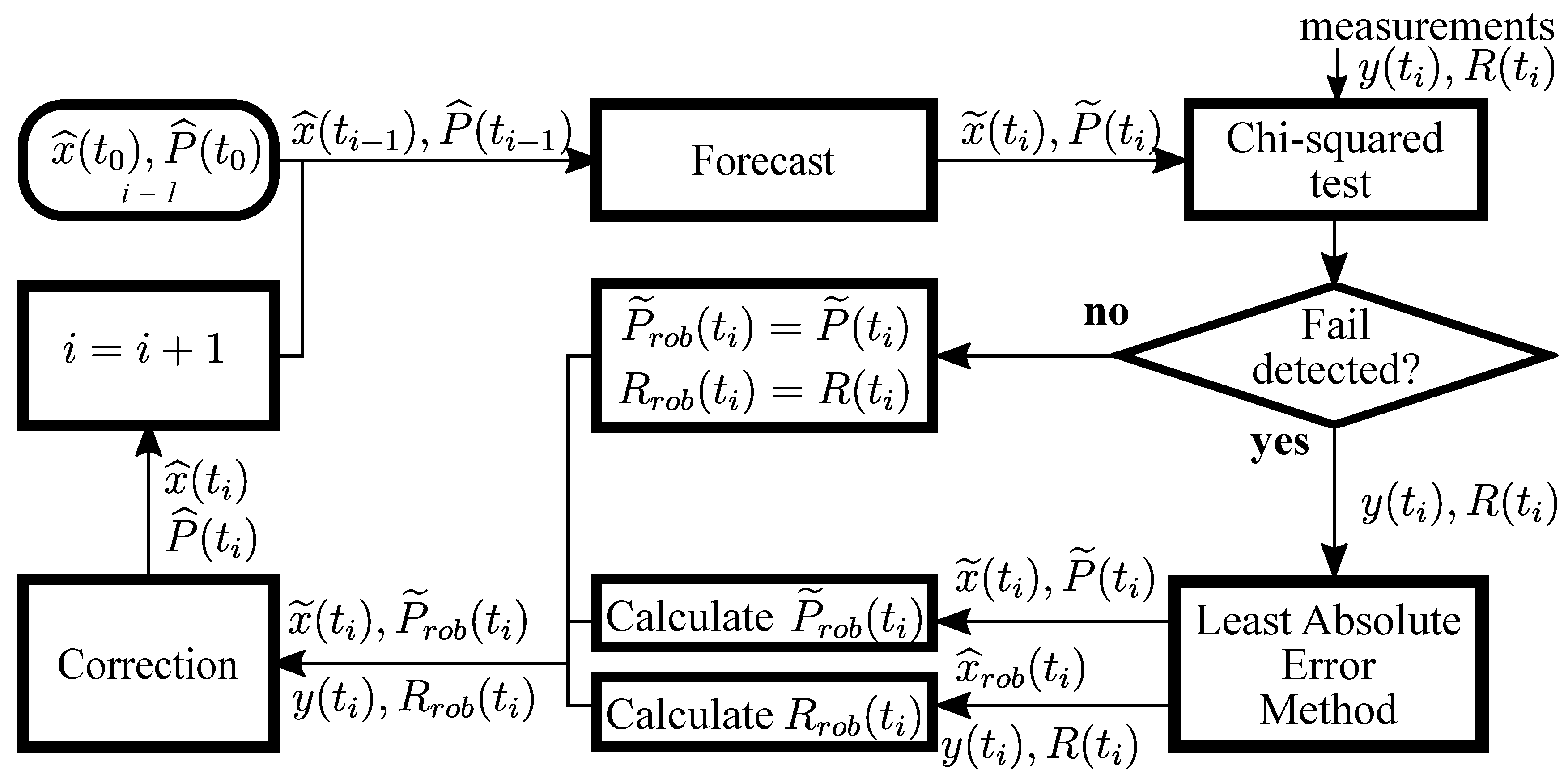
The robust filtering method proposed in this article is a superstructure over the Kalman filter. The main idea of the modification consists in the robust estimation and chi-squared test used together to control the measurement covariance matrix and the prediction covariance matrix. It is assumed that the determinants of these matrices can only increase. A procedure for testing and calculating covariance matrices is added between the prediction and correction steps. The scheme of the algorithm is shown on the Figure 3. The following sections will discuss the general methods underlying the algorithm. A more detailed description of the algorithm as it applied to the data fusion problem is presented in the Section 4.

3.1. Least Modulus Method

The goal of the least modulus method is to minimize L 1 -norm vector of errors. L 1 -norm of a vector is calculated as the sum of the absolute values of its elements. Consider the system of linear equations
z d = H d x + ϵ d ,
where H d is the observation matrix, x is a vector of estimated parameters, ϵ d is the measurement errors, z d is the measurement vector (dimension of z is greater than dimension of x). Estimate x ^ L 1 of x vector by the least modulus method is given by
x ^ L 1 = arg min x i = 1 n ( z d , ( i ) H d , ( i , : ) x )
provided that the measurement errors are independent and have the unit variance
E ϵ d ϵ d T = I .
Here z d , ( i ) is i-th element of vector z d , and H ( i , : ) is the i-th row vector of H matrix. Index d emphasizes the requirement that the vector ϵ d has to be decorrelated.
The idea of applying the method of least modules in the filtering problem is to estimate the current state by current measurements y ( t i ) and prediction of the state from the previous step x ˜ ( t i ) . The combination of the measurements an prediction vectors into one vector is called the extended measurement vector
z e ( t i ) = y ( t i ) T , x ˜ ( t i ) T T , C e ( t i ) = R ( t i ) 0 ( m × n ) 0 ( n × m ) P ˜ ( t i ) ,
where C e is covariance matrix of extended dimension measurements vector z e . Taking into account the dynamics equations we have
z e ( t i ) = H e x ( t i ) + ϵ ( t i ) , H e ( t i ) = H ( t i ) T , I ( n × n ) T ,
where ϵ ( t i ) is a vector of random variables with covariance matrix c o v ( ϵ ( t i ) , ϵ ( t i ) ) = C e ( t i ) .
The Cholesky decomposition L L T = c h o l ( C e ( t i ) ) for the covariance matrix of the extended measurement vector gives the decorrelated transformation:
z d ( t i ) = H d ( t i ) x ( t i ) + ϵ d ( t i ) = L 1 z e ( t i ) , H d ( t i ) = L 1 H e ( t i ) , ϵ d ( t i ) = L 1 ϵ ( t i ) ,
moreover
c o v ( ϵ d ( t i ) , ϵ d ( t i ) T ) = L 1 c o v ( ϵ ( t i ) , ϵ ( t i ) T ) L T = L 1 C e L T = L 1 L L T L T = I .
So we reduce our task to (10). In [40] it is recommended to use the proposed algorithm on personal computer. Since the prediction errors are not correlated with the measurement errors, the matrix L can be sought in the form:
L = L y 0 0 L x , L 1 = L y 1 0 0 L x 1 .
The approach to this minimization problem consists in using of the least square method proposed in [33,35,36] to obtain M-estimation. This method does not give an exact solution to the L 1 -minimization problem. The smaller the parameter c in (2), the closer the estimate to L 1 -optimal will be. However, a decrease in c leads to an increase in the convergence time.
Moreover, in [41] it is indicated that when solving the L 1 -minimization problem, the iterative least squares method has numerical instability. It needs to choose a convergence criterion. In [37,42] it was shown that problem (10) is reduced to a linear programming problem. Its solution which can be obtained by more efficient algorithms than the iterative least squares method. The function to be minimized is represented as
i = 1 n ϵ d ( i ) = i = 1 n ϵ 1 ( i ) + i = 1 n ϵ 2 ( i ) min
with constraints
H d , I ( n × n ) , I ( n × n ) · x ϵ 1 ϵ 2 = z d , ϵ 1 ( i ) 0 , ϵ 2 ( i ) 0 , i = 1 , , n .
To amend the efficiency of the algorithm in [43] the transition to the dual form of the problem is carried out (15) and (16)
i = 1 n z d ( i ) b i 1 max
for a system
H d T b = i = 1 n H d ( i , 1 ) i = 1 n H d ( i , m ) , 0 b ( i ) 2 , i = 1 , , n ,
To solve the problem (17) and (18) the simplex method is applied. Detailed description of the algorithm of L 1 -optimization can be found in [43]. This method provides an accurate solution despite the fact that it does not require significant computing resources. This particular method was used in this work.
After solving the problem by the method of least modules, the posterior residuals are calculated:
Δ z ( t i ) = L y 1 ( y ( t i ) H ( t i ) x ^ L 1 ) ,
Δ x ( t i ) = L x 1 ( x ˜ ( t i ) x ^ L 1 ) .
These residuals are used further to calculate the covariance matrices in case of failure detection.

3.2. Chi-Square Test for Failure Detection

In the normal operation of the system the distribution of measurement errors and prediction errors are assumed to be Gaussian with zero mathematical expectation. Otherwise we will assume that the error of the corresponding measurement has a nonzero mathematical expectation. Consider two competing hypotheses
H 0 : E z d ( t i ) = H d ( t i ) x ( t i ) , H 1 : E z d ( t i ) = H d ( t i ) x ( t i ) + A Δ ,
where A is the coefficient matrix (variance model), Δ are parameters of the deviation model. Taking into account that c o v ( ϵ d ( t i ) , ϵ d ( t i ) T ) = I , statistics suitable for testing hypotheses can be obtained in the form [44]
T = z d T B k ( B k T B k ) 1 B k T z d ,
where rank ( B k ) = ( m + n ) n = m , m is the dimension of the measurements vector, n is the state vector dimension, ( m + n ) – dimension of the extended vector of measurements and B k T H d = 0 . The B k matrix can be obtained through the QR decomposition of the H d matrix:
Q k , B k R k 0 ( m n ) × n ) = q r ( H d ( t i ) ) .
To implement QR decomposition, it is recommended to use the algorithm given in [40].
Depending on the accepted hypothesis, the statistics (21) will have the uncentered chi-squared distribution with m degrees of freedom and different values of the bias [44,45]:
H 0 : T χ 2 ( m , 0 ) ; H 1 : T χ 2 ( m , λ ) .
Here λ is the bias parameter calculated depending on the accepted failure model. In accordance with the Neumann-Pearson lemma the criterion of the next form is the most powerful criterion for choosing hypotheses
H 0 : T c ( m ) ; H 1 : T > c ( m ) ;
where the threshold value c ( m ) is calculated as the value of the argument of the distribution function χ 2 ( m , 0 ) , at which this function is equal to the given value of the errors probability of the first kind η :
c ( m ) = F χ 2 1 ( m , η , 0 ) .
The probability of type II errors is calculated as
β = F χ 2 ( c ( m ) , m , λ ) ,
where F χ 2 ( c ( m ) , m , λ ) is the value of the probability function of the uncentered χ 2 -distribution with m degrees of freedom and non-centrality parameter λ in the point c ( m ) . The value of the non-centrality parameter, taking into account (13) is calculated according to [44]:
λ = z d T B k T A ( A T B k B k T A ) 1 A T B k z d .
The unit matrix A = I is used for failure detection. Then the application of the criterion (22) solves the problem of failure detection with a minimum value of the probability of type II errors at λ = c ( m ) :
β min = F χ 2 ( c ( m ) , m , c ( m ) ) .
In practice, this probability is limited from above by the value β T H in accordance with the requirements for the system. The case when β min > β T H means that the system configuration in principle cannot provide a sufficiently low level of Type II errors.

3.3. Calculation of the Measurements Covariance Matrix

Depending on whether a failure is detected (accepted hypothesis H 1 ) or not (hypothesis accepted H 0 ), the estimate of the measurements covariance matrix is calculated
R r o b ( t i ) = L y D y L y T ,
where L y L y T = c h o l ( R ( t i ) ) , and D y is diagonal matrix whose elements are calculated by posterior residuals (19):
D y , ( j , j ) = ρ ( Δ z ( j ) ) , if H 1 , 1 otherwise
for j = 1 , , q m ( q m is the dimension of the measurements vector). Measurement residual vector Δ z is calculated according to (19). Form of the function ρ must be chosen so that the condition ρ ( x ) > 1 is carried out only with the probability of a false alarm α , provided that the hypothesis H 0 is true. An analytical solution to such a problem is beyond the scope of this study, therefore, an empirical piecewise function is used:
ρ ( x ) = 1 , if | x | < c , x 2 c 2 + 2 c k 1 exp [ k ( c | x | ) ] , if | x | c .
The parameter c is calculated depending on the specified false alarm probability in accordance with (23) for m = 1 , parameter k > 0 is customizable. For small values of k the solution will approach to the robust estimate (2). At large values of k the sensitivity of the estimate to large measurement discrepancies decreases.

3.4. Calculating the Predictive Covariance Matrix

It is assumed that the dynamic noise of the system n ( t i 1 , t i ) is generated by a multidimensional Wiener random process:
n ( t i 1 , t i ) = 0 t i t i 1 F ( t i 1 , t i 1 + τ ) B S d w ( τ ) .
Here w ( τ ) is the Wiener process of q w dimension, matrix S is the diagonal positive definite matrix of q w × q w dimension, B is q x × q w dimension matrix, where q x is the state vector dimension. For this definition, the dynamic noise covariance matrix can be represented as:
Q ( t i 1 , t i , s ) = j = 1 q w s ( j ) 0 t i t i 1 F ( τ ) B ( : , j ) ( B ( : , j ) ) T F T ( τ ) d w ( j ) ( τ ) .
Here s ( j ) is the j-th element of vector s equal to j-th diagonal element of matrix S 2 , B ( : , j ) is the j-th column vector of the matrix B and F ( τ ) for brevity means F ( t i 1 , t i 1 + τ ) .
It is assumed that the dynamic noise parameters s are given. We will calculate the covariance matrix in the form:
P ˜ r o b ( t i ) = P ˜ ( t i ) + Q ( t i 1 , t i , a s ) ,
where the value of the vector of dynamic noise parameters a s is determined from the condition:
tr L x D x L x T P ˜ ( t i ) = tr Q ( t i 1 , t i , a s ) .
Matrix D x is calculated in similar way as D y :
D x , ( j , j ) = ρ ( Δ x ( j ) ) , if H 1 , 1 otherwise
Vector of the residuals of the prior state and the posterior robust estimate Δ x is calculated according to (20), and the function ρ defined in (25).
In general, the solution to the Equation (29) relative to s may not be unique, then an empirical approach should be used. One of the possible methods was used in numerical experiments for this work (see Section 5).

4. Application of the Robust Filter in the Data Fusion Problem

In the previous section a description of the general robust filtering algorithm was given. Let us consider now the application of this algorithm for solving a specific problem.
For aircraft navigation at the approach stage the following measurement sources are used:
  • INS (horizontal coordinates),
  • altimeters (radio or barometric) with double redundancy,
  • landing systems (as a source of spherical coordinates).
The INS correction is performed according to an open circuit, which is shown in the Figure 4.

4.1. System Model

To reduce the dimension of the problem navigation in the horizontal channel is carried out separately from the vertical channel. It allows to use two parallel filters with lower dimension instead of one filter with a large dimension of the state vector.
The model of the system in the horizontal channel is the model of the error dynamics of the strapdown INS. Accurate nonlinear models of INS errors exist (see [16,23]). We will use a linear system to describe the dynamics of INS errors to simplify the prolem. In continuous time the model represents a system of stochastic differential equations:
d x h ( t ) = A h x h ( t ) d t + B h S h d w ( t ) ,
A h = 0 1 0 0 0 0 0 0 0 0 0 1 0 0 0 0 , B h = 0 0 1 0 0 0 0 1 , S h 2 = s h 0 0 s h
Vector components x h have the following physical meaning:
  • x h , ( 1 ) is INS error in the north direction (m),
  • x h , ( 2 ) is INS speed error in the north direction (m/s),
  • x h , ( 3 ) is INS error in the eastern direction (m),
  • x h , ( 4 ) is INS speed error in the east direction (m/s),
In the vertical channel, the model of the system dynamics is the aircraft motion model:
d x v ( t ) = A v x v ( t ) d t + B v S v d w ( t ) ,
A v = 0 1 0 0 0 0 0 0 0 0 0 1 0 0 0 0 , B v = 0 0 0 1 1 0 0 0 0 1 0 1 , S v 2 = s v , ( 1 ) 0 0 0 s v , ( 2 ) 0 0 0 s v , ( 3 )
Vector x v r t has the following physical meaning:
  • x v r t , ( 1 ) is height according to altimeter data (m),
  • x v r t , ( 2 ) is vertical speed according to altimeter data (m/s),
  • x v r t , ( 3 ) is height according to the landing system (m),
  • x v r t , ( 4 ) is vertical speed according to the indications of the landing system (m/s),
The discrete time model of the system takes the form:
x h ( t i ) = F ( Δ t ) x h ( t i 1 ) + n h ( Δ t ) , x v ( t i ) = F ( Δ t ) x v ( t i 1 ) + n v ( Δ t ) ,
F ( Δ t ) = 1 Δ t 0 0 0 1 0 0 0 0 1 Δ t 0 0 0 1 ,
Q = ( Δ t 3 ) / 3 ( Δ t 2 ) / 2 ( Δ t 2 ) / 2 Δ t , Q 1 = Q 0 ( 2 × 2 ) 0 ( 2 × 2 ) Q , Q 2 = Q Q Q Q , Q 3 = Q 0 ( 2 × 2 ) 0 ( 2 × 2 ) 0 ( 2 × 2 ) , Q 4 = 0 ( 2 × 2 ) 0 ( 2 × 2 ) 0 ( 2 × 2 ) Q ,
where Δ t = t i t i 1 and
E n h ( Δ t ) n h T ( Δ t ) = Q h ( Δ t , s h ) = s h Q 1 , E n v ( Δ t ) n v T ( Δ t ) = Q v ( Δ t , s v ) = s v , ( 1 ) Q 2 + s v , ( 2 ) Q 3 + s v , ( 3 ) Q 4 .

4.2. Measurements Model

The landing system makes measurements in spherical coordinates:
α ( t i ) = arctan E ( t i ) N ( t i ) + Δ α ( t i ) , γ ( t i ) = arctan U ( t i ) E ( t i ) 2 + N ( t i ) 2 + Δ γ ( t i ) , r ( t i ) = E ( t i ) 2 + N ( t i ) 2 + U ( t i ) 2 + Δ r ( t i ) ,
where α ( t i ) is the azimuth angle, γ ( t i ) is the elevation angle, r ( t i ) is the slant range; Δ α ( t i ) , Δ γ ( t i ) , Δ r ( t i ) are the measurements errors; E , N , U the aircraft coordinates in the local normal coordinate system E ( t i ) is the east coordinate, N ( t i ) is the north coordinate, U ( t i ) is the vertical coordinate. To avoid nonlinearities in the observation matrix we will use the pseudo-measurement method [24,26]:
m n ( i l s ) ( t i ) = N ( t i ) + Δ m n ( t i ) = r ( t i ) cos ( γ ( t i ) ) cos ( α ( t i ) ) , m u ( i l s ) ( t i ) = U ( t i ) + Δ m u ( t i ) = r ( t i ) sin ( γ ( t i ) ) , m e ( i l s ) ( t i ) = E ( t i ) + Δ m e ( t i ) = r ( t i ) cos ( γ ( t i ) ) sin ( α ( t i ) ) .
During normal operation of the landing system the angular measurement errors do not exceed several degrees and given the fact that the standard approach is carried out along the glide path with an inclination angle of not more than 4 degrees, an approximate expression for the covariance measurement matrix can be written:
E [ Δ m ( i l s ) ( Δ m ( i l s ) ) T ] = M Σ M T ,
M = cos ( γ ) cos ( α ) sin ( γ ) cos ( α ) sin ( α ) sin ( γ ) cos ( γ ) 0 cos ( γ ) sin ( α ) sin ( γ ) sin ( α ) cos ( α ) , Σ = σ Δ r 2 0 0 0 r 2 σ Δ a 2 0 0 0 r 2 σ Δ a 2
where σ Δ r is the RMS error of range measurement, σ Δ a is the RMS error of angular measurements.
From the inertial system, measurements are received in a geographic coordinate system (latitude and longitude), which can be converted to Cartesian coordinates N U E . We denote these coordinates by m n ( i n s ) , m e ( i n s ) . Then the input of the filter in the horizontal channel will receive the differences between the pseudo-measurements of the landing system and the INS measurements:
y h , ( 1 ) ( t i ) = m n ( i l s ) ( t i ) m n ( i n s ) ( t i ) , y h , ( 2 ) ( t i ) = m e ( i l s ) ( t i ) m e ( i n s ) ( t i ) ,
which are related to the state vector through the relation:
y h ( t i ) = H h x h + ϵ h , H h = 1 0 0 0 0 0 1 0
and the covariance matrix
R h ( t i ) = E ϵ h ϵ h T = M h Σ M h T , M h = cos ( γ ) cos ( α ) sin ( γ ) cos ( α ) sin ( α ) cos ( γ ) sin ( α ) sin ( γ ) sin ( α ) cos ( α ) .
It is implied here that the INS measurement noise is negligible.
Altimeter measurements and landing system measurements are available in the vertical channel:
y v , ( 1 ) ( t i ) = m u ( a l t 1 ) = x v , ( 1 ) + ϵ v , ( 1 ) , y v , ( 2 ) ( t i ) = m u ( a l t 2 ) = x v , ( 1 ) + ϵ v , ( 2 ) , y v , ( 3 ) ( t i ) = m u ( i l s ) = x v , ( 3 ) + ϵ v , ( 3 ) ,
with observation matrix:
H v = 1 0 0 0 1 0 0 0 0 0 1 0
and the covariance matrix
R v ( t i ) = E ϵ h ϵ h T = σ a 2 0 0 0 σ a 2 0 0 0 M v Σ M v T , M v = sin ( γ ) cos ( γ ) 0 .

4.3. Data Fusion Algorithm

In the final form the integration algorithm consists of the following steps:
  • Set constant robust filter parameters: false alarm probability η in the Equation (23), weight coefficient k in the Equation (25), dynamic noise intensity s h and s v for (34) calculation, RMS of measurements σ Δ r , σ Δ a , σ a .
  • Set the initial state of the filter in the horizontal channel x ^ h ( t 0 ) , P ^ h ( t 0 ) and the initial state of the filter in the vertical channel x ^ v ( t 0 ) , P ^ v ( t 0 ) .
  • The following steps are repeated as measurements arrive. Calculate state prediction:
    x ˜ h ( t i ) = F ( Δ t ) x h ( t i 1 ) , P ˜ h ( t i ) = F ( Δ t ) P ^ h ( t i 1 ) F T ( Δ t ) + Q h ( Δ t , s h ) , x ˜ v ( t i ) = F ( Δ t ) x v ( t i 1 ) , P ˜ v ( t i ) = F ( Δ t ) P ^ v ( t i 1 ) F T ( Δ t ) + Q v ( Δ t , s v ) .
  • Calculate test statistics (21) and apply the criterion (22). If the hypothesis H 0 is accepted, then go to step 9 with P ˜ h , r o b ( t i ) = P ˜ h ( t i ) , P ˜ v , r o b ( t i ) = P ˜ v ( t i ) , R h , r o b ( t i ) = R h ( t i ) , R v , r o b ( t i ) = R v ( t i ) .
  • If the hypothesis H 1 is accepted (i.e., a failure is detected), calculate a robust least modulus state estimate (10) and residuals (19) and (20) for horizontal channel: Δ z h ( t i ) , Δ x h ( t i ) ; and for vertical channel Δ z v ( t i ) , Δ x v ( t i ) .
  • Using residuals Δ z h ( t i ) and Δ z h ( t i ) calculate accordingly R h , r o b and R v , r o b by Formula (24).
  • Using residuals Δ x h ( t i ) calculate matrix D h by Formula (24). Using Cholesky decomposition L h L h T = c h o l ( P ˜ h ( t i ) ) calculate the estimate of the prediction matrix
    P ˜ h , r o b ( t i ) = P ˜ h ( t i ) + s Q 1 , s = tr L h D h L h T P ˜ h ( t i ) tr Q 1 ,
    where Q 1 is calculated by the Formulas (33).
  • Using residuals Δ x v ( t i ) calculate matrix D v by Formula (24). Using Cholesky decomposition L v L v T = c h o l ( P ˜ v ( t i ) ) calculate the estimate of the prediction matrix
    P ˜ v , r o b ( t i ) = P ˜ v ( t i ) + s 1 Q 3 + s 2 Q 4 , s 1 = subtr L v D v L v T P ˜ v ( t i ) ( 1 : 2 ) tr Q 3 , s 2 = subtr L v D v L v T P ˜ v ( t i ) ( 3 : 4 ) tr Q 4 ,
    where subtr A ( i : j ) is the trace of a submatrix formed from columns and rows with indices from i to j square matrix A. Matrices Q 3 , Q 4 are calculated by the Formulas (33).
  • The calculated estimates of the covariance matrices are used to obtain the state estimate in accordance with the Kalman filter correction step:
    K h = P ˜ h , r o b ( t i ) H h T ( H h P ˜ h , r o b ( t i ) H h T + R h , r o b ) 1 , x ^ h ( t i ) = x ˜ h ( t i ) + K h ( y h H h x ˜ h ( t i ) ) , P ^ h ( t i ) = ( I K h H h ) P ˜ h , r o b ( t i ) ,
    where y h and H h are calculated by the Formulas (39) and (40). The estimate for the vertical channel is calculated in the same way.

5. Discussion of Test Results

The main goal of this study was to develop an estimation algorithm that is robust against abnormal errors in measurement channels. Our flying model was relatively large and rather expensive, so we use a set of redundant sensors as a source of possible errors to develop reliable algorithms for their use in the event of failure of some sensors such as altimetemer and or locator used for correcting the standard INS. The actual landing is carried out using a standard INS, supported by a satellite positioning system, which serves as a source of real data on the position and velocities of the aircraft. Backup sensors data serve to debug the estimation algorithm and check its performance in case of abnormal errors. This approach allows to minimize the risk of losing the aircraft. Since landing is one of the most critical phases of flight, our research team has conducted a series of different experiments over the past several years with various additional sensors, including video cameras [2,3] and ground-based optical and radio beacons-radars [4]. The series of experiments performed recently were made on the basis of the optical flow registration [46,47]. To simplify the experiments we used the sensors data registered during the flight to simulate them later in the software and to update by various algorithms. Comparison of known and suggested algorithms is presented in this section.
To demonstrate the properties of suggested robust algorithm numerical simulation was carried out, where the measurements were processed with a discrete Δ t = 0.1 s. The following algorithm settings were used:
false alarm probability (23) η = 10 4 ,
penalty function parameter (25) k = 0.4 .
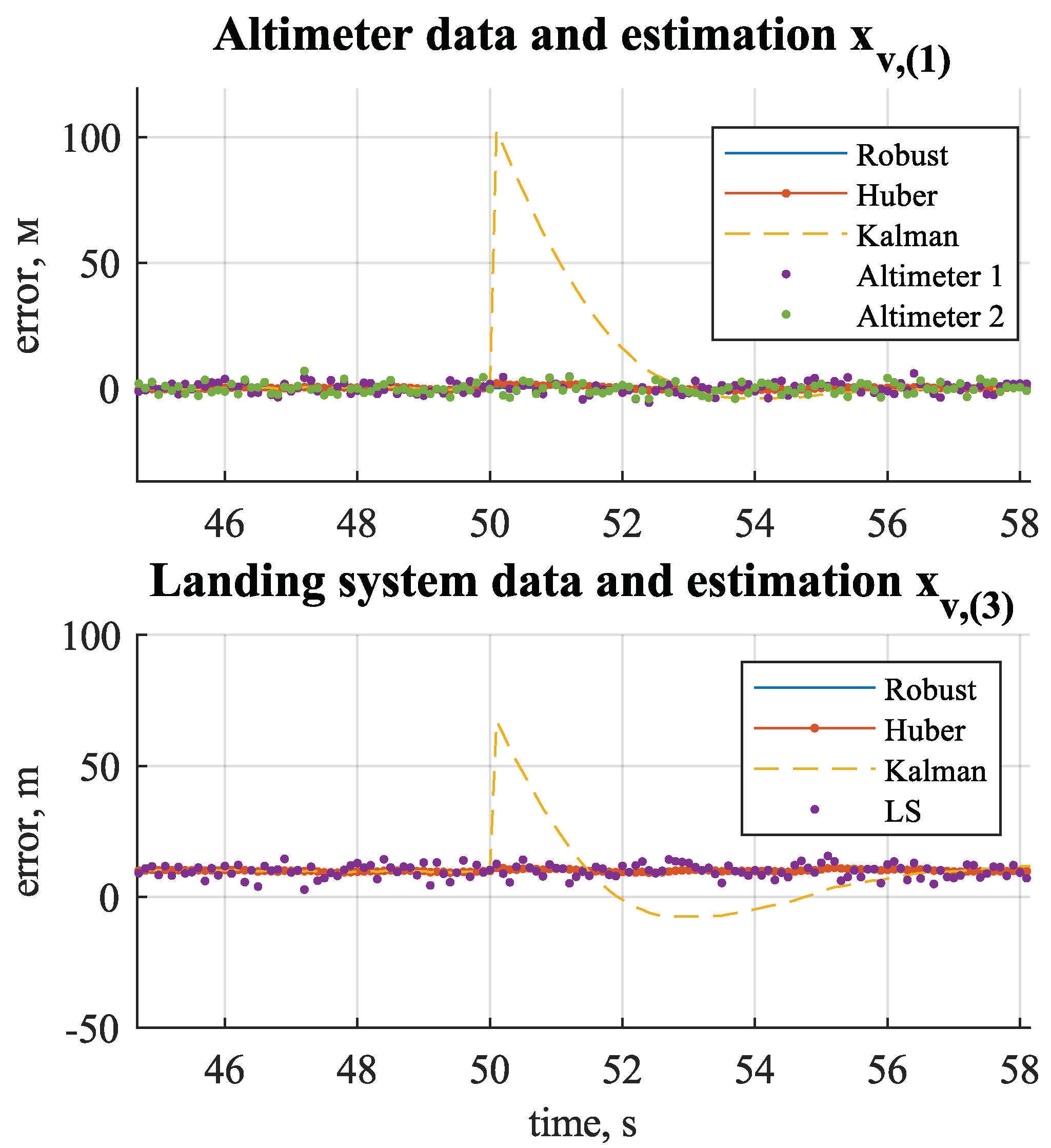
On the Figure 5 it is shown the filter response to the stepwise measurement error in the vertical channel. On the Figure 6 the filter response to impulse measurement error is shown. Unlike the optimal Kalman filter, the robust filter is insensitive to impulse noise, and in the case of a step change in the measurement error the robust filter is insensitive to measurement errors for some time, but then quickly «attracts» to the measurements. In this case, the transient time is less than for the optimal Kalman filter. For comparison, the figures also show the graph of the robust estimate (2).
Changing the coefficient k allows us to adjust the smoothness of the transition process. Values which are close to zero make the transient look like a robust estimate (2). Larger values make the transient jump with a time delay. Figure 7 shows how the shape of the transient changes with the coefficient k changes. The simulation results of the case when an anomalous step error appears only in one of the redundant sources are shown on the Figure 8. The developed algorithm is resistant to this type of error.
We should demonstrate the disadvantages of the proposed algorithm. They must be taken into account when used in critical cases. Figure 9a,b show a case of a slow divergence of measurements from redundant altimeters. In such kind of situations the robust integration algorithm chooses, roughly speaking, one of the sensors and further monitors its measurements, reducing the weight of the other sensor. The choice is made randomly, which introduces an element of uncertainty in the behavior of the system in such situations.
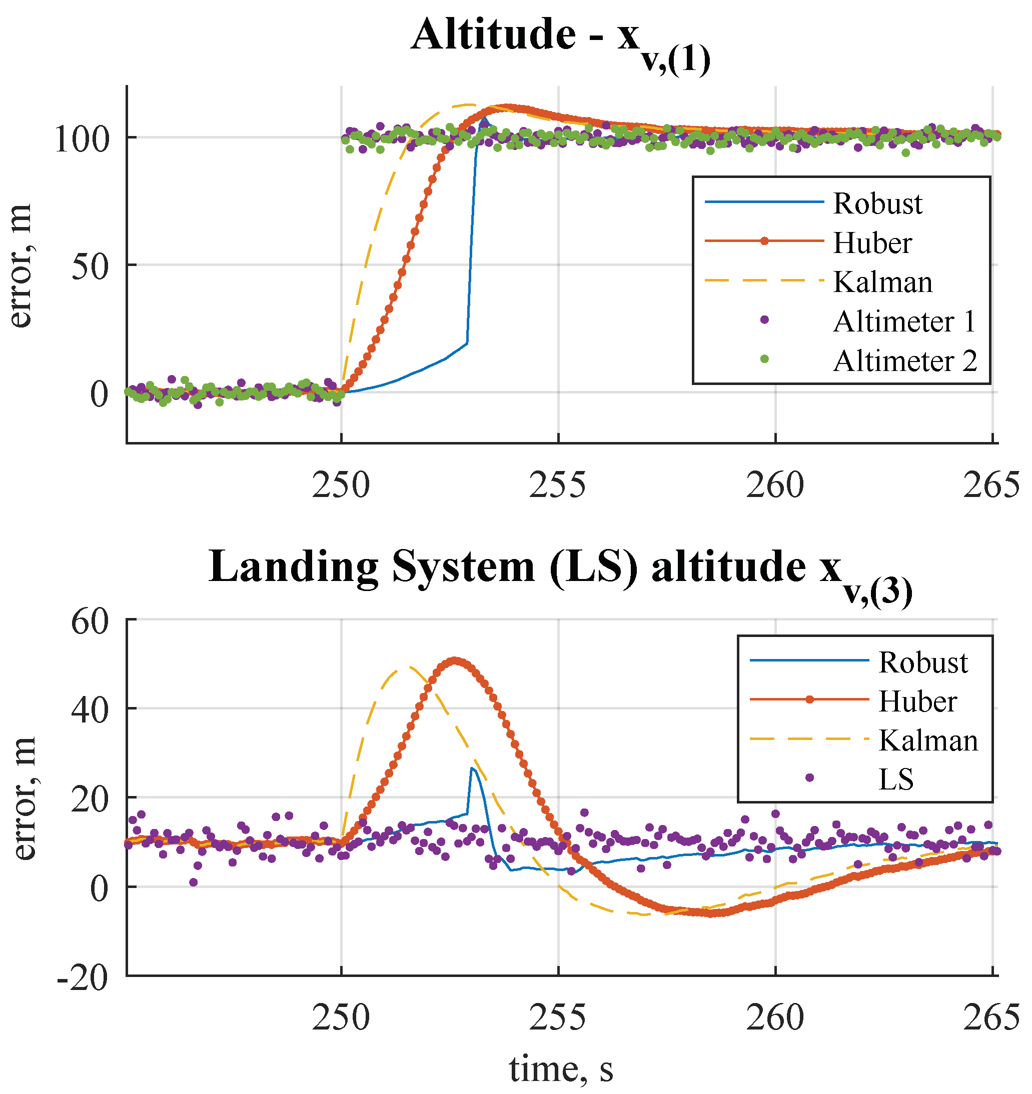
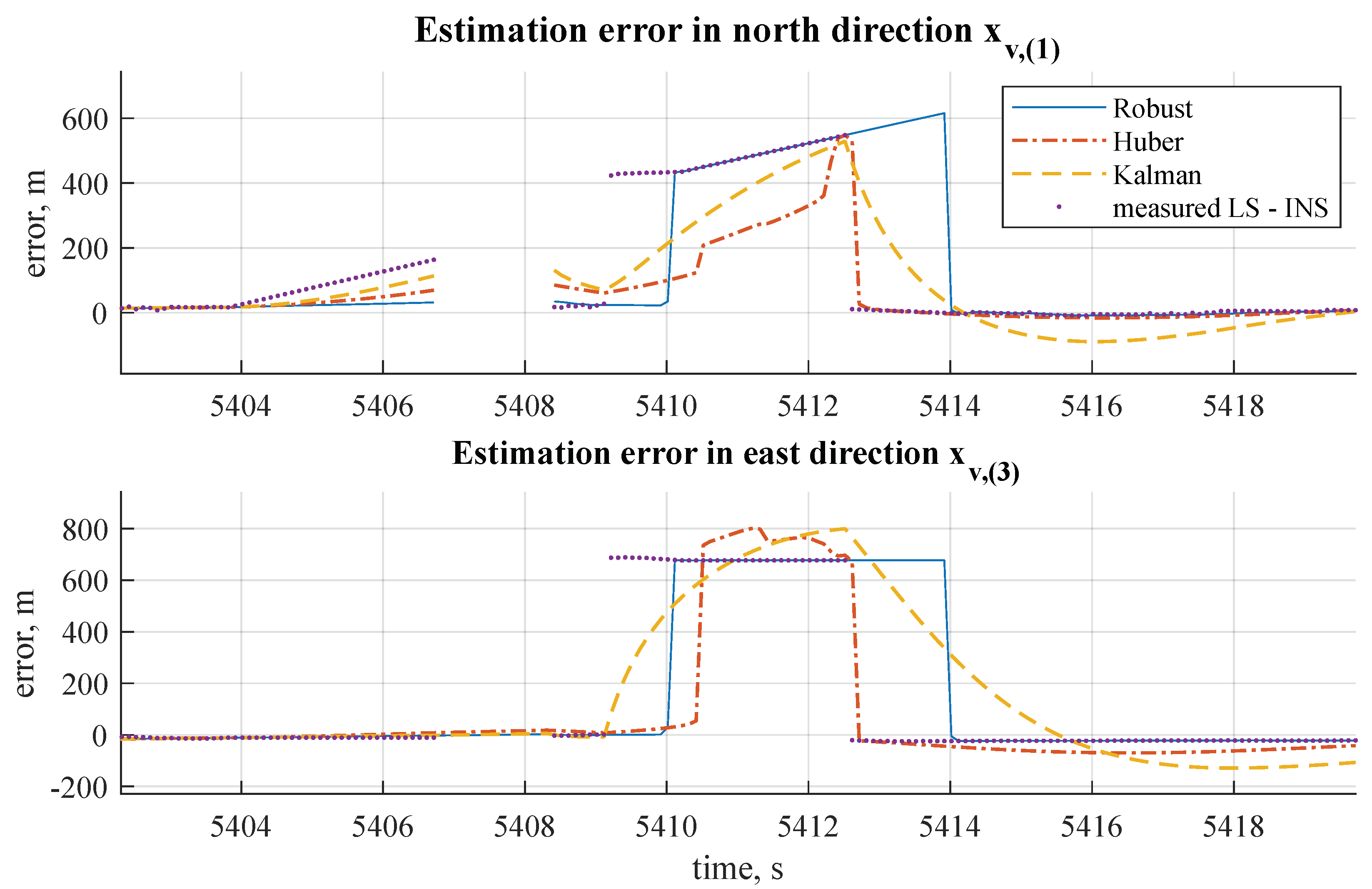
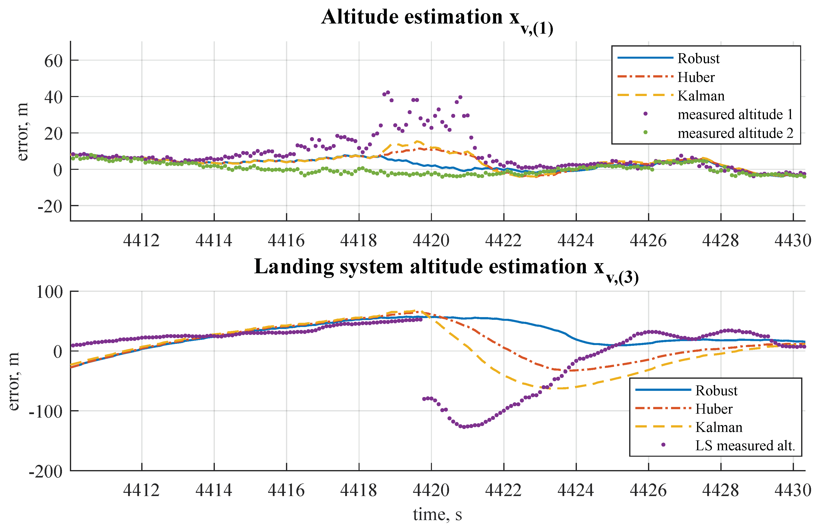
The results of processing of the real measurements registered during the test flight are shown on Figure 10, Figure 11 and Figure 12. It is necessary to indicate that the position measurements were made using INS sensors and a ground locator of the type [18,19] that determines the angular position and range to the aircraft. Using a locator results in a special type of anomalous error, such as jumping from the main to the side lobe of the antenna directional pattern, which may be observed on Figure 11 and Figure 12. In the horizontal channel the data of the locator and the airborne INS are combined. In the vertical channel of the locator and radio altimeter. Figure 12 shows an approach segment where abnormal errors are present in the measurements of one of the altimeters. Simultaneously, there is a jump in the dimensions of the landing system. The estimate obtained by the robust algorithm is less responsive to abnormal measurement errors. On the Figure 10 a real situation is shown where the measurements of the landing system contained a complex error. The graphs show that the estimate obtained using the developed algorithm coincides with the optimal Kalman estimate in normal operation, and at the same time, moreover, the estimate is resistant to outliers in measurements. On the Figure 11 another real situation is shown where the measurements of the landing system contained a U-shaped error.

6. Conclusions

The data fusion problem for nonlinear measurements of the landing system, airborne INS and airborne altimeters was considered. It was shown that the classical data fusion methods based on the Kalman filter are not suitable for solving the problem, since they can reduce the reliability of the navigation solution in systems with redundant sensors. To solve the problem a robust filtering algorithm was developed, the principal feature of which is the estimate stability to abnormal measurements. The recurrence of the estimate is ensured by using the Kalman filter relations; along with filtering, a procedure for testing hypotheses about the presence of anomalous errors in measurements and in the state predicting is proposed. When the threshold set by the false alarm probability is exceeded, the filter switches to the robust estimation mode, in which the prediction and measurement covariance matrices are estimated based on the least modulus method.
The test results show that the developed algorithm, on the one hand, is resistant to short-term emissions in measurements, on the other hand, it provides a fast transient process. The last property is important, since there is a nonzero probability of missing an alarm and measurements with a biased error can fall into the filter, which will lead to a bias in the estimate. If at some time the measurement errors return to their normal unbiased form, the algorithm should quickly recover to track new measurements.
The developed algorithm does not protect against all types of abnormal measurement errors. It was shown that if the system uses double redundancy of sensors and in one of the redundant sensors the error expectation increases slowly over time, the algorithm selects one of the sensors and then monitors only its measurements. Moreover, this choice is random. To get rid of this uncertainty, either additional measurements should be used, or a special procedure for detecting disputable situations should be provided. The development of such a procedure is the subject of further research. However, it should be noted that this type of error is much less common than short-term spikes or noise amplification in measurements of one of the redundant sensors. The results of testing on real data show that the developed algorithm can provide a reliable assessment of navigation parameters across all available information, while ensuring the detection and isolation of individual sensor failures.

Author Contributions

Conceptualization, K.K. and B.M.; software, K.K.; writing—review and editing, A.M. All authors have read and agreed to the published version of the manuscript.

Funding

The work of B. Miller and A. Miller is partially funded according to the Russian Government Program of Competitive Growth of Kazan Federal University, 18 Kremlyovskaya str, Kazan, 420008, Russian Federation.

Conflicts of Interest

The authors declare no conflict of interest.

Abbreviations

The following abbreviations are used in this manuscript:
INSInertial Navigation System
GNSSGlobal Navigation Satellite System
UKFUnscented Kalman filter
EKFExtended Kalman Filter

References

  1. You, Y.; Cao, J.; Zhou, W. A Survey of Change Detection Methods Based on Remote Sensing Images for Multi-Source and Multi-Objective Scenarios. Remote Sens. 2020, 12, 2460. [Google Scholar] [CrossRef]
  2. Karpenko, S.; Konovalenko, I.; Miller, A.; Miller, B.; Nikolaev, D. UAV Control on the Basis of 3D Landmark Bearing-Only Observations. Sensors 2015, 15, 29802–29820. [Google Scholar] [CrossRef] [PubMed] [Green Version]
  3. Konovalenko, I.; Miller, A.; Nikolaev, D.; Miller, B. UAV Navigation On The Basis Of The Feature Points Detection On Underlying Surface. In Proceedings of the 29th European Conference on Modelling and Simulation, ECMS 2015; Valeri, M.M., Ed.; Technical University of Sofia: Sofia, Bulgaria, 2015; pp. 500–505. [Google Scholar]
  4. Miller, A.B.; Miller, B.M. Stochastic control of light UAV at landing with the aid of bearing-only observations. In Proceedings of the SPIE 9875, Eighth International Conference on Machine Vision (ICMV 2015) (8 December 2015), Barselona, Spain, 19–20 November 2015. [Google Scholar] [CrossRef]
  5. Tao, F.; Zhou, T. Identification of Urban Functional Areas by Coupling Satellite Images and Taxi GPS Trajectories. Remote Sens. 2020, 12, 2449. [Google Scholar]
  6. Arce, S.; Cory, A.V.; Hammond, J.; Newell, V.; Janson, J.; Franke, K.W.; Hedengren John, D. Automated 3D Reconstruction Using Optimized View-Planning Algorithms for Iterative Development of Structure-from-Motion Models. Remote Sens. 2020, 12, 2169. [Google Scholar] [CrossRef]
  7. Farella, E.M.; Torresani, A.; Remondino, F. Refining the Joint 3D Processing of Terrestrial and UAV Images Using Quality Measures. Remote Sens. 2020, 12, 2873. [Google Scholar] [CrossRef]
  8. Pham, H.X.; La, H.M.; Feil-Seifer, D.; Nguyen, L.V. Autonomous UAV Navigation Using Reinforcement Learning. arXiv 2018, arXiv:1801.05086. [Google Scholar]
  9. Amer, K.; Samy, M.; Shaker, M.; Elhelw, M. Deep Convolutional Neural Network-Based Autonomous Drone Navigation. arXiv 2019, arXiv:1905.01657. [Google Scholar]
  10. Hodge, V.J.; Hawkins, R.; Alexander, R. Deep Reinforcement Learning for Drone Navigation Using Sensor Data. Neural Comput. Appl. 2020. [Google Scholar] [CrossRef]
  11. Maier, A.; Kiesel, S.; Trommer, G.F. Performance analysis of federated filter for SAR/TRN/GPS/INS integration. Gyroscopy Navig. 2011, 2, 293–300. [Google Scholar] [CrossRef]
  12. Hu, G.; Gao, S.; Zhong, Y.; Gao, B.; Subic, A. Modified federated Kalman filter for INS/GNSS/CNS integration. Proc. IMechE Part G J. Aerosp. Eng. 2016, 230, 30–44. [Google Scholar] [CrossRef]
  13. Wright, M.A.; Horowitz, R. Particle-filter-enabled real-time sensor fault detection without a model of faults. In Proceedings of the 2017 IEEE 56th Annual Conference on Decision and Control (CDC), Melbourne, VIC, Australia, 12–15 December 2017; pp. 5757–5763. [Google Scholar] [CrossRef] [Green Version]
  14. Gao, B.; Hu, G.; Gao, S.; Zhong, Y.; Gu, C. Multi-Sensor Optimal Data Fusion Based on the Adaptive Fading Unscented Kalman Filter. Sensors 2018, 18, 488. [Google Scholar] [CrossRef] [Green Version]
  15. Veremeenko, K.K.; Zheltov, S.Y.; Kim, N.V.; Kozorez, D.A.; Krasil’shchikov, M.N.; Sebryakov, G.G.; Sypalo, K.I.; Chernomorsky, A.I. Modern Information Technologies in the Tasks of Navigation and Guidance of Unmanned Maneuverable Aerial Vehicles; Fizmatlit: Moscow, Russia, 2009. (In Russian) [Google Scholar]
  16. Salychev, O.S. Mems-Based Inertial Navigation: Expectations and Reality; Bauman Moscow State Technical University: Moscow, Russia, 2012. [Google Scholar]
  17. Kaplan, E.; Hegarty, C. Understanding GPS: Principles and Applications; ARTECH HOUSE: Boston, MA, USA; London, UK, 2006. [Google Scholar]
  18. Sierra Nevada Corporation. Tactical Automatic Landing System. Available online: www.sncorp.com (accessed on 20 November 2020).
  19. Ground-Based Navigation—Instrument Landing System (ILS). Available online: https://www.faa.gov/ (accessed on 20 November 2020).
  20. OPATS Laser Based Landing Aid for Unmanned Aerial Vehicles. RUAG—Aviation Products Switzerland. Available online: www.ruag.com/aviation (accessed on 20 November 2020).
  21. Konovalenko, I.; Kuznetsova, E.; Miller, A.; Miller, B.; Popov, A.; Shepelev, D.; Stepanyan, K. New Approaches to the Integration of Navigation Systems for Autonomous Unmanned Vehicles (UAV). Sensors 2018, 18, 3010. [Google Scholar] [CrossRef] [Green Version]
  22. Sasiadek, J.Z.; Hartana, P. Sensor Fusion for Navigation of an Autonomous Unmanned Aerial Vehicle. In Proceedings of the IEEE lnternational Conference on Robotics and Automation; Program Chair Kimon Valavanis: New Orleans, LA, USA, 2004; Volume 4, pp. 4029–4034. [Google Scholar]
  23. Titterton, D.; Weston, J.L.; Weston, J. Strapdown Inertial Navigation Technology Stevenage, UK; Institution of Electrical Engineers: Reston, VA, USA, 2004. [Google Scholar]
  24. Lin, X.; Kirubarajan, T.; Bar–Shalom, Y.; Maskell, S. Comparison of EKF, Pseudomeasurement and Particle Filters for a Bearing-only Target Tracking Problem. Proc. SPIE 2002, 4728, 240–250. [Google Scholar]
  25. Julier, S.J.; Uhlmann, J.K.; Durrant-Whyte, H.F. A New Approach for Filtering Nonlinear Systems. In Proceedings of the 1995 American Control Conference-ACC’95, Seattle, WA, USA, 21–23 June 1995; pp. 1628–1632. [Google Scholar]
  26. Miller, A.B.; Miller, B.M. Tracking of the UAV trajectory on the basis of bearing-only observations. In Proceedings of the 53rd IEEE Conference on Decision and Control; Andrew, R.T., Ed.; IEEE: Los Angeles, CA, USA, 2014; pp. 4178–4184. [Google Scholar]
  27. Huber, P.J. Robust Statistics; Wiley Series in Probability and Mathematical Statistics; John Wiley & Sons: New York, NY, USA, 1981. [Google Scholar]
  28. Hampel, F.R.; Ronchetti, E.M.; Rousseeuw, P.J.; Stahel, W.A. Robust Statistics: The Approach Based on Influence Function; John Wiley & Sons: New York, NY, USA, 1986. [Google Scholar]
  29. Bosov, A.V.; Pankov, A.R. Robust Recurrent Estimations of Processes in Stochastic Systems. Autom. Remote Control 1992, 53, 1395–1402. [Google Scholar]
  30. Pearson, R.K. Outliers in Process Modeling and Identification. IEEE Trans. Control. Syst. Technol. 2002, 10, 55–63. [Google Scholar] [CrossRef]
  31. Markovich, N. Nonparametric Analysis of Univariate Heavy-Tailed Data: Research and Practice; John Wiley & Sons: Hoboken, NJ, USA, 2007. [Google Scholar]
  32. Gustafsson, F. Particle filter theory and practice with positioning applications. IEEE Aerosp. Electron. Syst. Mag. 2010, 25, 53–82. [Google Scholar]
  33. Cao, L.; Qiao, D.; Chen, X. Laplace L1 Huber based cubature Kalman filter for attitude estimation of small satellite. Acta Astronaut. 2018, 148, 48–56. [Google Scholar] [CrossRef]
  34. Kotz, S.; Kozubowski, T.J.; Podgorski, K. The Laplace Distribution and Generalizations; Springer Science+Business Media: New York, NY, USA, 2001. [Google Scholar]
  35. Koch, K.R.; Yang, Y. Robust Kalman Filter for Rank Deficient Observation Models. J. Geod. 1998, 72, 436–441. [Google Scholar] [CrossRef]
  36. Chang, G.; Liu, M. M-estimator-based Robust Kalman Filter for Systems with Process Modeling Errors and Rank Deficient Measurement Models. Nonlinear Dynam. 2015, 80, 1431–1449. [Google Scholar] [CrossRef]
  37. Abdelmalek, N.N. On the Discrete Linear L1 Approximation and L1 Solutions of Overdetermined Linear Equations. J. Approx. Theory 1974, 11, 38–53. [Google Scholar] [CrossRef]
  38. Liptser, R.S.; Shiryaev, A.N. Random Process Statistics; Springer: New York, NY, USA, 1978. [Google Scholar]
  39. Gelb, A. Applied Optimal Estimation; MIT Press: Cambridge, MA, USA, 2001. [Google Scholar]
  40. Hogben, L. Handbook of Linear Algebra, 2nd ed.; New York Imprint; Chapman and Hall/CRC Press: New York, NY, USA, 2013. [Google Scholar]
  41. Armstrong, R.D.; Frome, E.L. A Comparison of Two Algorithms for Absolute Deviation Curve Fitting. J. Am. Stat. Assoc. 1976, 71, 328–330. [Google Scholar] [CrossRef]
  42. Barrodale, I.; Roberts, F. An Improved Algorithm for Discrete L1 Linear Approximation. SIAM J. Numer. Anal. 1973, 10, 839–848. [Google Scholar] [CrossRef]
  43. Abdelmalek, N.N. An Efficient Method for the Discrete Linear L1 Approximation Problem. Math. Comput. 1975, 29, 844–850. [Google Scholar]
  44. Teunissen, P.J.G. Distributional Theory for the DIA Method. J. Geod. 2018, 92, 59–80. [Google Scholar] [CrossRef]
  45. Xu, C.; Rui, X.; Song, X.; Gao, J. Generalized Reliability Measures of Kalman Filtering for Precise Point Positioning. J. Syst. Eng. Electron. 2013, 24, 699–705. [Google Scholar] [CrossRef]
  46. Popov, A.; Miller, A.; Miller, B.; Stepanyan, K. Optical flow and inertial navigation system fusion in the UAV navigation. In Unmanned/Unattended. Sensors and Sensor Networks XII, Proceedings of the 998606 (2016) SPIE Security + Defence, Edinburgh, UK, 26–29 September 2016; SPIE Digital Library: Bellingham, WA, USA, 2016. [Google Scholar] [CrossRef]
  47. Miller, B.; Miller, A.; Popov, A.; Stepanyan, K. UAV Landing Based on the Optical Flow Videonavigation. Sensors 2019, 19, 1351. [Google Scholar] [CrossRef] [Green Version]
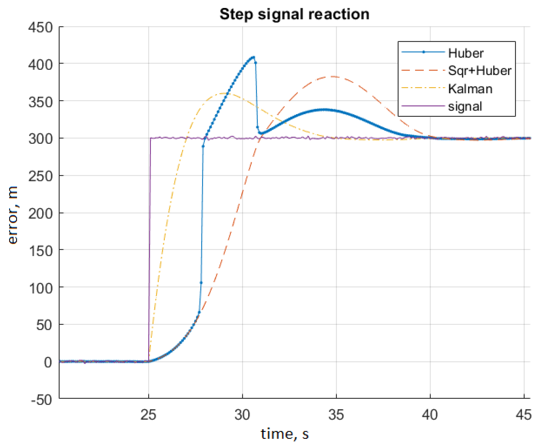
Figure 1. Transients for different filtering methods.
Remotesensing 12 03849 g001
Figure 2. Estimate response to step error in measurements from a backup measurements source.
Remotesensing 12 03849 g002
Figure 3. Robust Algorithm Scheme.
Remotesensing 12 03849 g003
Figure 4. The inertial navigation systems (INS) correction scheme.
Remotesensing 12 03849 g004
Figure 5. Filter response to step measurements. «Robust»—the proposed robust algorithm. «Huber»—M score.
Remotesensing 12 03849 g005
Figure 6. Response of filters to impulse surge at the moment of time t = 50 s. «Robust»—the proposed robust algorithm. «Huber»—M score.
Remotesensing 12 03849 g006
Figure 7. Filter response to step measurements. «Robust»—the proposed robust algorithm. «Huber»—M score.
Remotesensing 12 03849 g007
Figure 8. Filter response to step error in backup altimeter measurements. «Robust»—the proposed robust algorithm. «Huber»—M score.
Remotesensing 12 03849 g008
Figure 9. Modelling of a slow divergence of altimeters measurements. In sample (a) robust filter tracks second altimeter measurements. In sample (b) robust filter tracks first altimeter measurements. The choice is made equiprobably.
Remotesensing 12 03849 g009
Figure 10. Filter response to anomalous complex shape error in landing system measurements. «Robust»—the proposed robust algorithm. «Huber»—M score.
Remotesensing 12 03849 g010
Figure 11. Filter response to abnormal U-shape error in landing system measurements. «Robust»—the proposed robust algorithm. «Huber»—M score.
Remotesensing 12 03849 g011
Figure 12. Filters response to abnormal vertical channel errors. «Robust»—the proposed robust algorithm. «Huber»—M score.
Remotesensing 12 03849 g012
Publisher’s Note: MDPI stays neutral with regard to jurisdictional claims in published maps and institutional affiliations.