Improved Prototypical Network Model for Forest Species Classification in Complex Stand

Abstract

Deep learning has become an effective method for hyperspectral image classification. However, the high band correlation and data volume associated with airborne hyperspectral images, and the insufficiency of training samples, present challenges to the application of deep learning in airborne image classification. Prototypical networks are practical deep learning networks that have demonstrated effectiveness in handling small-sample classification. In this study, an improved prototypical network is proposed (by adding L2 regularization to the convolutional layer and dropout to the maximum pooling layer) to address the problem of overfitting in small-sample classification. The proposed network has an optimal sample window for classification, and the window size is related to the area and distribution of the study area. After performing dimensionality reduction using principal component analysis, the time required for training using hyperspectral images shortened significantly, and the test accuracy increased drastically. Furthermore, when the size of the sample window was 27 × 27 after dimensionality reduction, the overall accuracy of forest species classification was 98.53%, and the Kappa coefficient was 0.9838. Therefore, by using an improved prototypical network with a sample window of an appropriate size, the network yielded desirable classification results, thereby demonstrating its suitability for the fine classification and mapping of tree species.

1. Introduction

Information regarding tree species functions as the fundamental data for forest management. The accurate identification of forest tree species is crucial for inventorying forest resources, estimating carbon storage on forest grounds, effectively managing forest resources, and for the timely monitoring of species diversity. Numerous continuous narrow spectral bands and high spatial resolution of hyperspectral image (HSI) can provide continuous spectral information for each pixel [1], which plays a crucial role in the accurate classification of tree species [2,3]. Forest-type identification is a vital aspect of the application of hyperspectral imagery [4,5,6]. HSI provide abundant spectral information. However, they are prone to the Hughes [7] phenomenon whereby the classification accuracy first increases and then decreases as the number of bands in the analysis increases. Therefore, for the dimensionality reduction of airborne hyperspectral data, the representative spectral–spatial features should be extracted [8]. Feature transformation is a dimensionality reduction method in which multiple feature values of the original high-dimensional feature space are mapped onto a low-dimensional space, based on a specific principle and using certain mathematical operations, similar to the principal component analysis (PCA) method [9]. Sidike et al. [10] used a progressively expanded neural network to gradually classify HSI. They also used the PCA dimensionality reduction method to reduce computational complexity and avoid dimensional disasters, by extracting features for each band. Another method is band selection [11], which is based on the original information of the image. This method selects some of the most representative bands from the original band according to a specific criterion, similar to the random forest (RF) [12,13] method. Wu et al. [14] eliminated hyperspectral features using the RF method and further improved the classification accuracy and performance of the support vector machine classifier. However, regardless of whether feature transformation or band selection is employed, information loss owing to dimensionality reduction is inevitable. Therefore, the impact of dimensionality reduction on specific data should be investigated. The fine spectral and spatial characteristics of airborne hyperspectral data are beneficial for tree species identification. However, the problem of reduced classification efficiency and information redundancy caused by a large data volume is particularly prominent. Notably, it limits the application of airborne HSI in regional classification mapping [15,16]. Thus, exploring new classification methods and seeking a balanced solution between making full use of effective information, improving classification time efficiency, and ensuring classification accuracy are crucial for the regional mapping of complex forest stands and tree species. However, only a few studies have been conducted in this regard.

Deep learning can extract advanced and semantic features [17,18]. Moreover, its objective function directly focuses on classification and automatically completes feature extraction from the data and the training of the classifier [19]. Hence, deep learning has become a research hotspot for HSI classification [20,21,22]. However, the topic is still challenging. In the application of deep learning classification, the ability to achieve feature representation relies on a large number of training samples [23]. Deep learning classification of small samples may cause network overfitting, which is the network model performs very well on the training set, and nearly perfectly predicts and distinguishes all the data, but shows substantial differences on the new test set. Commonly used methods to solve network overfitting include increasing the number of samples, adding regularization to the network structure or dropout to the network structure, and terminating model training early. Among them, regularization [24] and dropout [25] are effective solutions to eliminate model overfitting. In particular, L2 regularization can be regarded as the regularization of the loss function, which is used to impose restrictions on some parameters in the loss function. Dropout refers to allowing the activation value of a certain neuron to cease working with a certain probability during forward propagation. Only a specific number of neurons are involved in each training cycle, while other neurons are not included. In forests, sample collection is hindered because of the complex terrain and stand structure. Further, the heterogeneity of the structure, composition of the tree species, and similarity of the image features render sample labeling tasks difficult for the classification of forest tree species. Therefore, the problem of tree species classification based on a deep learning method for small-sample sets should be addressed urgently [26,27,28]. Pan et al. [29] designed a new network called vertex component analysis network for deep feature extraction from the smoothed HSI. Moreover, this method achieves higher accuracy when the number of training samples is not abundant. Xu et al. [30] proposed a random patches network for HSI classification, which directly regards the random patches obtained from the image as the convolution kernels without any training.

The convolutional neural network (CNN) is one of the most popular deep learning methods, exhibiting significant advantages in image classification [31]. The significant improvement in computing power in recent years has resulted in the rapid development of many CNNs, such as AlexNet [32], VGGNet [33], MobilenetV1 [34], and MobilenetV2 [35]. However, these CNNs have complex network structures, which include a large number of layers, such as convolutional layers and pooling layers. This complex network structure consumes significant amounts of valuable computing and memory resources and wastes training time. Recent studies on HSI classification have proved that the three-dimensional convolutional neural network (3D-CNN) model is superior to other CNNs [36], and it can solve high-dimensional classification problems for large data sets with high spatial and spectral resolution [37]. The prototypical network (PrNet) has been proven to be effective for solving small-sample classification [38]. PrNets learn a metric space in which classification can be performed by computing distances to prototype representations of each class. It can allow neurons to use prior knowledge to adjust the model according to the new task [39]. Specifically, a simple classifier is generated dynamically in the new training stage, and the core embedding is fixed after the training [40]. The PrNet is a metric learning approach. The basic idea of metric learning is to learn the distance function between images [41]. The PrNet extracts features from the image, calculates the average value of the image embedding for each category, and obtains the prototype of each category. The classification can be performed by calculating the distance of the image embedded in the prototype. Thus, the distance function is crucial. In this regard, Euclidean distance is the most effective distance function [42].

The PrNet has a simple network structure and is suitable for small-sample learning problems. Based on the large and fine spatial spectrum characteristics of the airborne HSIs, in this study, we use the PrNet to classify tree species. Due to the differences in quantities and characteristics of the information obtained from different data sources, the data source affects the classification performance of the PrNet. Therefore, based on the volume and characteristics of information from a specific data source, we study how different training samples affect the classification accuracy and efficiency of the PrNet classification, which is a crucial aspect. Moreover, under the same experimental conditions, we compare the classification performance of 3D-CNN and PrNet to verify whether PrNet has advantages in small-sample conditional classification. The major contributions of the proposed PrNet can be summarized as follows:

• Improve the structure and parameter adjustment of a PrNet such that it is more suitable for the tree species classification of a small sample of airborne HIS.
• Analyze the effect of data dimensionality reduction on the classification accuracy and the network operation efficiency.
• Proposes a sample size suitable for PrNet to classify tree species of airborne HIS.

2. Materials and Methods

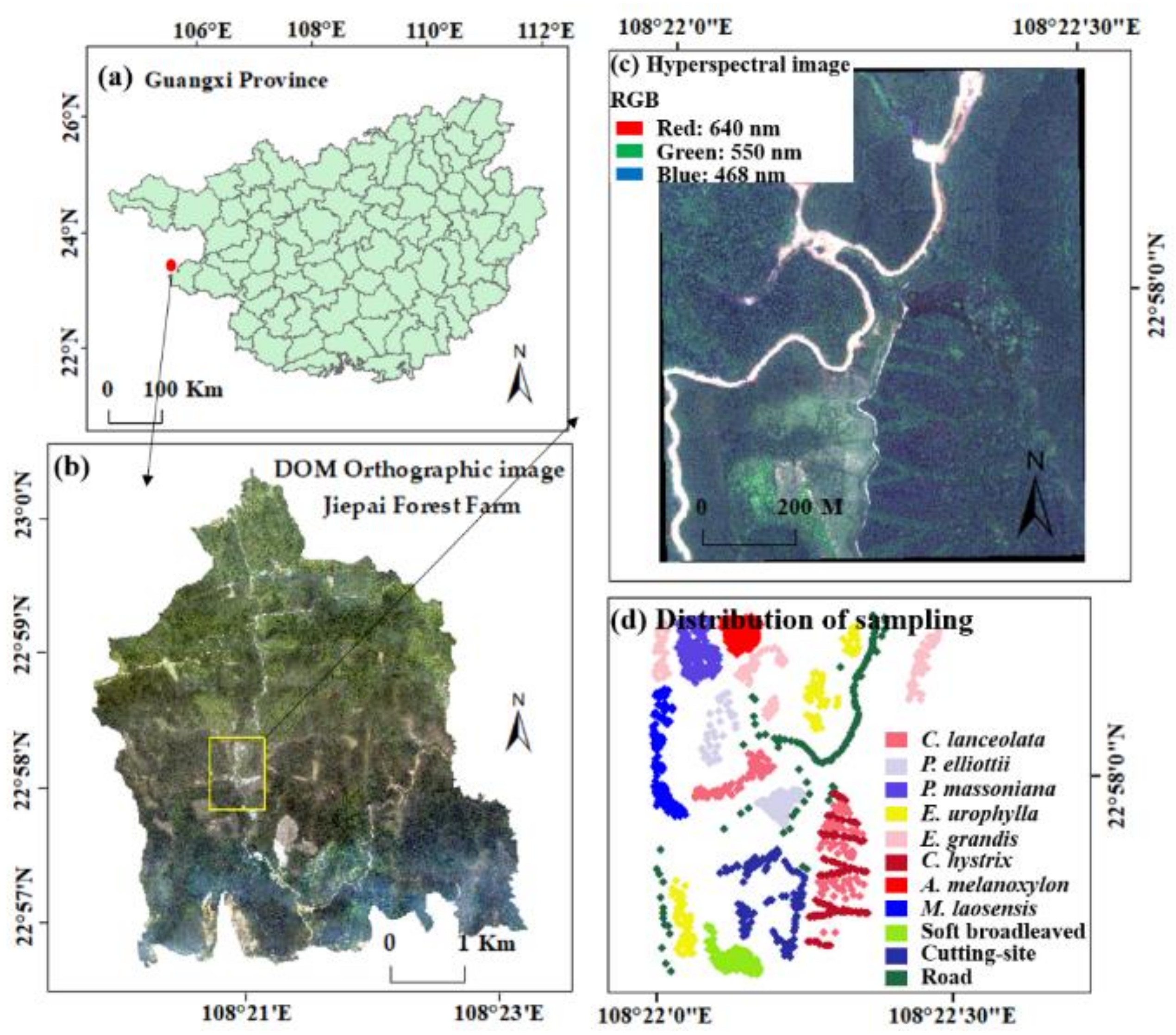
2.1. Study Area

The land area of the Gaofeng forest farm in Nanning City, Guangxi Province, China, is 59,000 hm². The complex forest stands and understory conditions pose challenges for tree species classification. In this study, the subfields of the Gaofeng forest farm (108°22′1″–108°22′30″ E, 22°57′42″–22°58′13″ N) were selected as the research area (Figure 1). The land area within the study area is 74.1 hm², the regional altitude is 149–263 m, and the landform types are hills and low mountains. The study area belongs to the south subtropical monsoon climate region. The annual average temperature is 21.6 °C, extreme maximum temperature is 40.0 °C, extreme minimum temperature is −2 °C, and accumulated temperature is 7500 °C. The average annual rainfall is 1304.2 mm, and the average relative humidity is 79%. The study area is dominated by middle-aged and near-mature forests. The study of remote sensing tree species classification in this area is crucial for the classification and mapping of forests with complex structures and compositions.

2.2. Classification System and Survey of Field Sample Points

The pure Cunninghamia lanceolata (C. lanceolata, CL) forest in the study area is a model forest that is undergoing natural transformation. Over the past 20 years, the region has adjusted the stand structure by gradually transforming the artificial pure forest into a coniferous and broadleaf forest to cultivate C. lanceolata (CL) and Castanopsis hystrix (C. hystrix, CH) large-diameter timber and to improve the economic benefits of the forest stand, forest quality, and ecology features. The study area also includes a demonstration garden of fast-growing and high-yielding tree species, with Eucalyptus robusta and Pinus as the main species [43]. In 2014, the Taxus chinensis and Manglietiastrum sinicum were intercropped under the canopy. However, because of the late planting time, the average stand height was between 1.5 and 0.78 m, which is generally located under the C. lanceolata (CL) and C. hystrix (CH) forest, and as a result, the optical remote sensing images cannot obtain the spectral reflectance features. Thus, 11 categories in the study area are used for classification, including nine main tree species, cutting sites, and roads. Coniferous species include C. lanceolata (CL), Pinus elliottii (P. elliottii, PE), and Pinus massoniana (P. massoniana, PM). The broadleaf species include Eucalyptus urophylla (E. urophylla, EU), Eucalyptus grandis (E. grandis, EG), C. hystrix (CH), Acacia melanoxylon (A. melanoxylon, AM), Mytilaria laosensis (M. laosensis, ML), and other soft broadleaf species (SB).

The field survey was conducted in the Gaofeng Forest Farm, between 16 January 2019 and 5 February 2019. First, Gaofen-2 satellite images were interpreted at a resolution of 1 m. According to the principle of uniform distribution, the plots were arranged for the area covered by remote sensing. Some areas with complex terrain could not be arranged into plots. Thus, 19 square survey plots of 25 m × 25 m each were delineated. Seven plots comprised pure C. lanceolata (CL) forests, three plots comprised E. urophylla (EU) forests, and three plots comprised E. grandis (EG) forests. The remaining six plots contained other stands and mixed forests. The tree species included C. lanceolata (CL), P. massoniana (PM), E. urophylla (EU), E. grandis (EG), and C. hystrix (CH). The position of individual trees was taken as the actual sample point. The data regarding the positions of individual trees consisted of two parts: the position within the plot, measured using a China Sanding STS-752 Series Total Station (Nanjing Hanzhong Mapping Equipment Co. Ltd., Jiangsu, China), and the position outside the plot, measured using a hand-held GPS (South Group, Guangzhou). The positioning accuracy of the sampling points is demonstrated in the work of Wu and Zhang [14]. For the categories with too many sample points, the edges of the sample points with an excessively dense distribution were removed to render the number of sample points for each feature category consistent and evenly distributed. For the categories with too few sample points, the points on the study area images were manually marked based on the field survey GPS positioning points and digital orthophoto map (DOM, resolution: 0.2 m). Hence, each category held 112 sample points, for a total of 1232 points (Figure 1).

2.3. Acquisition and Preprocessing of Hyperspectral Images

The airborne HSIs were acquired at noon under a cloudless sky on 13 January 2019 and 30 January 2019. The hyperspectral equipment was housed in a LiCHy system (Integrated Geospatial Innovations, Kreuztal, Germany) that integrates light detection and ranging (LiDAR), a charge-coupled device camera, an AISA Eagle II hyperspectral sensor, and an inertial measurement unit (IMU). The LiCHy system is a push broom imaging system, and it covers the spectral ranges from 400 to 1000 nm. The aircraft carrying the hyperspectral equipment had a flight speed of 180 km·h⁻¹, a relative altitude of 750 m, an absolute altitude of 1000 m, and a route spacing of 400 m. The HSIs were composed of a geometrically corrected radiance, including 125 bands with wavelengths ranging from 400.76 to 987.21 nm. The size of the hyperspectral imagery in the study area was 914 × 1056 × 125 (Height × Width × Band).

Table 1. Parameters of the hyperspectral sensors in the LiCHy system.

Hyperspectral: AISA Eagle II
Spectral resolution	3.3 nm	Spatial resolution	1 m
Angle of view	37.7°	Spatial pixels	1024
Instantaneous angle of view	0.646 mrad	Spectral sampling interval	4.6 nm
Focal length	18.5 mm	Bit depth	12 bits

summarizes the detailed parameters of the hyperspectral sensors.

This study used the MODTRAN 4+ radiation transfer model [44] supported by ENVI 5.3 to perform atmospheric correction on the HSIs. The model can correct the cascade effect caused by diffuse reflection and adjust the spectrum smoothing caused by artificial suppression. Due to the complex terrain of the study area, the remote sensing images were affected by the orientation of the sensor, the height and orientation of the sun, and uneven brightness values. Thus, terrain correction was performed on the HSIs based on the digital elevation model (DEM) generated from the synchronously acquired LiDAR data. Changes to the image radiance values caused by terrain fluctuation were eliminated so that the image better reflected the spectral characteristics of the ground. The Savitzky–Golay filter was used to smooth the spectral data to effectively remove the noise caused by various factors [45].

PCA and RF methods were used to reduce the dimensionality of the HSIs in the study area. After PCA dimension reduction, the first five principal components contained more than 99% of the information of all bands. Therefore, these components were used as the data sources after PCA dimension reduction. Furthermore, RF can calculate the importance of each frequency band and arrange them in descending order. Based on the average reduction accuracy, the difference between the importance values of the two adjacent bands in the first eight bands was >0.1. Starting from the ninth band, the difference between the importance values of the two adjacent bands was <0.1, indicating only a slight difference in importance when starting from the ninth band. Therefore, the first eight bands were used as the data sources after RF dimension reduction. These included Band 33 (546.05 nm), Band 34 (550.70 nm), Band 35 (546.05 nm), Band 36 (555.35 nm), Band 37 (564.68 nm), Band 71 (726.10 nm), Band 82 (779.13 nm), and Band 96 (846.88 nm).

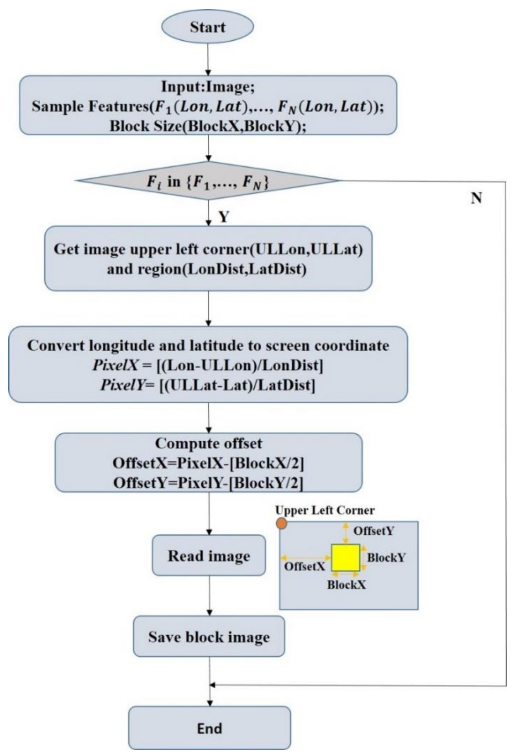
2.4. Sample Data Construction

The HSI, PCA dimension-reduced image (HSI_PCA), and RF dimension-reduced image (HSI_RF) were used as individual data sources. The open source geospatial data abstraction library framework was used to crop the sample data. First, the latitude and longitude coordinates of each measured sample point and their classification label attributes were read. Thereafter, the latitude and longitude coordinates were converted into screen coordinates (sample data are in pixels). The screen coordinates were used as input parameters to obtain the cropped area of the HSI data (Height × Width × Band, or H × W × B), and the sample was cropped from the data source according to a certain window size. The slice data were generated by creating an ENVI standard format file, which was used as the input data source of the PrNet. Figure 2 shows the flowchart of the sample data clipping algorithm [29]. The sample data were divided into training and test samples in ratios of 80% and 20%, respectively.

2.5. Prototypical Network Construction

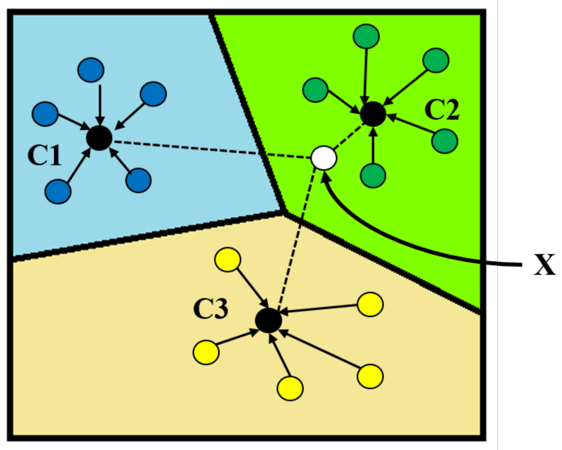
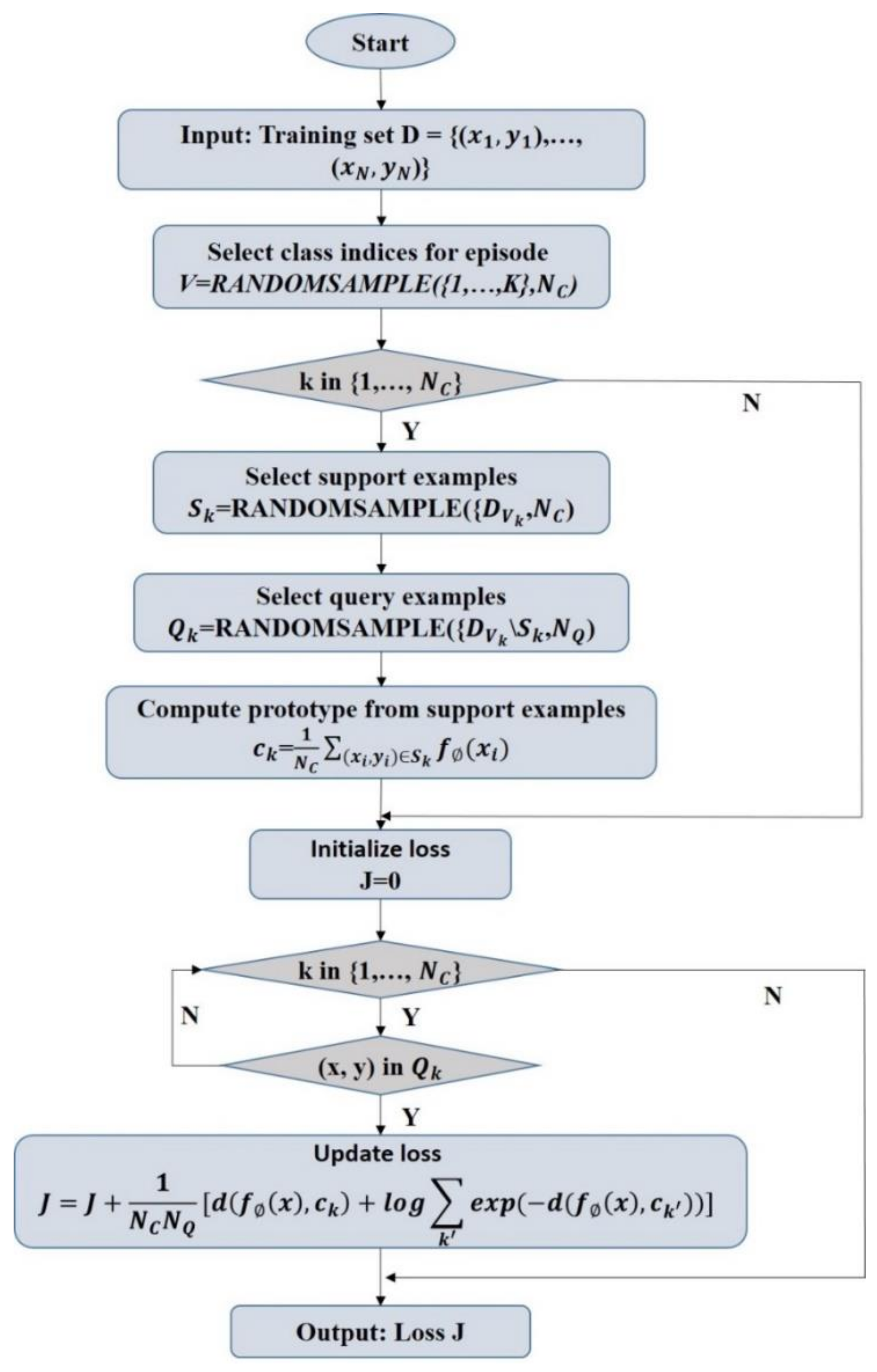
2.5.1. Prototypical Network Model

The classification principle of the PrNet is that the points of each class are clustered around a prototype. Specifically, the neural network learns the nonlinear mapping of the input to the embedding space and uses the average value of the support set as the prototype of its class in the embedding space. Next, the nearest class prototype is found to classify the embedded query points. Figure 3 shows the schematic representation of the PrNet [40]. The figure shows samples in the projection space with three categories (C1, C2, and C3). The distance between samples of the same category was relatively close. The average of these sample features was used as the category prototype (black dots in Figure 3). To perform classification on the unlabeled sample X, the sample was projected into the space, and the prototype closest to X was calculated. Finally, X was considered to be in the category represented by the prototype (C2).

In the PrNet classification, N samples are considered for the training set S, Equation (1), and each sample corresponds to a type of sample label.

$$S=\left\{\left(x_1,y_1\right),\left(x_2,y_2\right),\dots ,\left(x_N,y_N\right)\right\},$$

(1)

where x_i∈R^D is the D dimensional feature vector of a sample, y_i∈{1, …, K} is the corresponding sample label, and S_k serves as a training set with the sample label k. The training set of each class is further divided into a support set and a query set. The support set was used to calculate the prototype, and the query set was used to optimize the prototype. If there are A classes, and each class has B samples as the support set, it is A-way-B-shot.

The PrNet embeds the function f_∅R^D→R^M (∅ is the learning parameter), calculates the M dimension of each class, and represents c_k∈R^M as the class prototype. Each prototype is the average of the vectors obtained by the embedding function of the support set samples of its class Equation (2).

$$c_k=\frac{1}{\left|S_k\right|}{{\displaystyle \sum }}_{\left(x_i,y_i\right)ϵS_k}{f}_{\varnothing }\left(x_i\right),$$

(2)

Set the distance function as d: R^M × R^M→ [0, +∞]. In this study, the distance function is expressed as the square of the Euclidean distance ||z-z′||².The PrNet calculates the distance from the query, sets x to the prototypical in the projection of the embedded space through the distance function, and then uses the Softmax function to calculate the probability of a sample belonging to this category Equation (3).

$$p_{\varnothing }\left(y=k|x\right)=\frac{\exp \left(-d\left(f_{\varnothing }\left(x\right),c_k\right)\right)}{{{\displaystyle \sum }}_{k^{\prime }}\exp \left(-d\left(f_{\varnothing }\left(x\right),c_{k^{\prime }}\right)\right)},$$

(3)

The loss function uses a negative log-likelihood function Equation (4) and stochastic gradient descent (SGD) to minimize the loss function of the real category k and randomly select categories from the training set. Subsequently, a subset of the training set was selected as the support set within each category. Finally, one of the remaining categories was selected as a query point for training data input. Figure 4 shows the flowchart of the loss calculation algorithm for each training.

$$\mathrm{J}\left(\varnothing \right)=-\log p_{\varnothing }(y=k|x),$$

(4)

where N is the number of training set samples, K is the number of training set categories, N_C≤K is the number of categories for each training, N_S is the number of support set samples for each category, and N_Q is the number of samples in the query set of each category. In addition, RANDOMSAMPLE (S, N) represents a random and non-repetitive set of N elements selected from the set S.

2.5.2. Prototypical Network Classification Algorithm and Improvement

Slice data with a window size of S × S were used as the input data to the PrNet. The number of convolution blocks (Layer 1…Layer N, Layer last) in the architecture of the embedded function varies according to the size of the cropped data window. Each convolutional structure consists of a convolutional layer (Conv2d), batch normalization layer (Batch_norm), nonlinear activation function (Relu), and maximum pooling layer (Max_pool2d). The fully connected layer (Flatten) uses the output (1 × 1 × F) of the last convolutional structure as input and converts it into F eigenvalues (Figure 5). The Euclidean distance from the query set to each prototypical in the projection space was estimated, and the Softmax activation function Equation (3) was used to calculate the probability of a sample belonging to each category.

In this study, the output space dimension (F) of the convolutional layer was 64, and the size of the convolution kernel was 3 × 3. The size of the pooling core of the largest pooling layer was 2 × 2. This network structure produced a 64-dimensional output space (F). The same embedding function was used to operate the support set and query set. Both sets were then used as input parameters for loss and accuracy calculation. All models were trained using Adam-SGD, and the initial learning rate was 10⁻³. The learning rate was halved every 2000 training cycles. We employed the Euclidean distance as a metric function to train the PrNet.

In existing research on the recognition of text using PrNets, images of text are commonly rotated and scaled to increase the size of the training set [40,41]. This study classifies forest tree species without rotating and zooming the images, and a small training set may cause overfitting of the network. Therefore, we proposed an improved method to eliminate possible network overfitting. In the PrNet classification framework, the largest pooling layer of each convolutional structure was used to connect the next convolutional structure and provide its input. Therefore, L2 regularization (Kernel: L2) of the convolution kernel was added to the convolutional layer, and dropout (the probability of neuron deactivation is 1-Keep_prob) was added to the maximum pooling layer as an improved PrNet (IPrNet) to classify HSI. Equation (5) shows the loss calculation function of the training model IPrNet. The improved model was more generalized and not dependent on certain local features. Figure 5 presents the classification process.

$$L\left(\varnothing \right)=-\log p_{\varnothing }\left(y=k|x\right)+ {\alpha }_2{{\displaystyle \sum }}_w{w}^2,$$

(5)

where −logp_∅ (y = k│x) is the loss function, α₂ is the regularization coefficient, and w is the weight vector.

2.5.3. Accuracy Verification

The classification accuracy includes training accuracy and test accuracy. Training accuracy is expressed using last epoch accuracy (LEA), which is the average overall accuracy of each iteration. The test accuracy is expressed using the overall accuracy (OA), Equation (6) and the Kappa coefficient (Kappa), Equation (7).

$$\mathrm{OA}=\frac{{{\displaystyle \sum }}_{i=1}^n{X}_{ii}}{M},$$

(6)

$$\mathrm{Kappa}=\frac{M{{\displaystyle \sum }}_{i=1}^n{X}_{ii}-{{\displaystyle \sum }}_{i=1}^n{X}_{i+}\times X_{+i}}{M^2-{{\displaystyle \sum }}_{i=1}^n{X}_{i+}\times X_{+i}},$$

(7)

where X_ii is the number of correct classifications of a category in the error matrix, X_+i is the total number of true reference samples of that category, X_i+ is the total number of categories classified into this category, and M is the total number of samples.

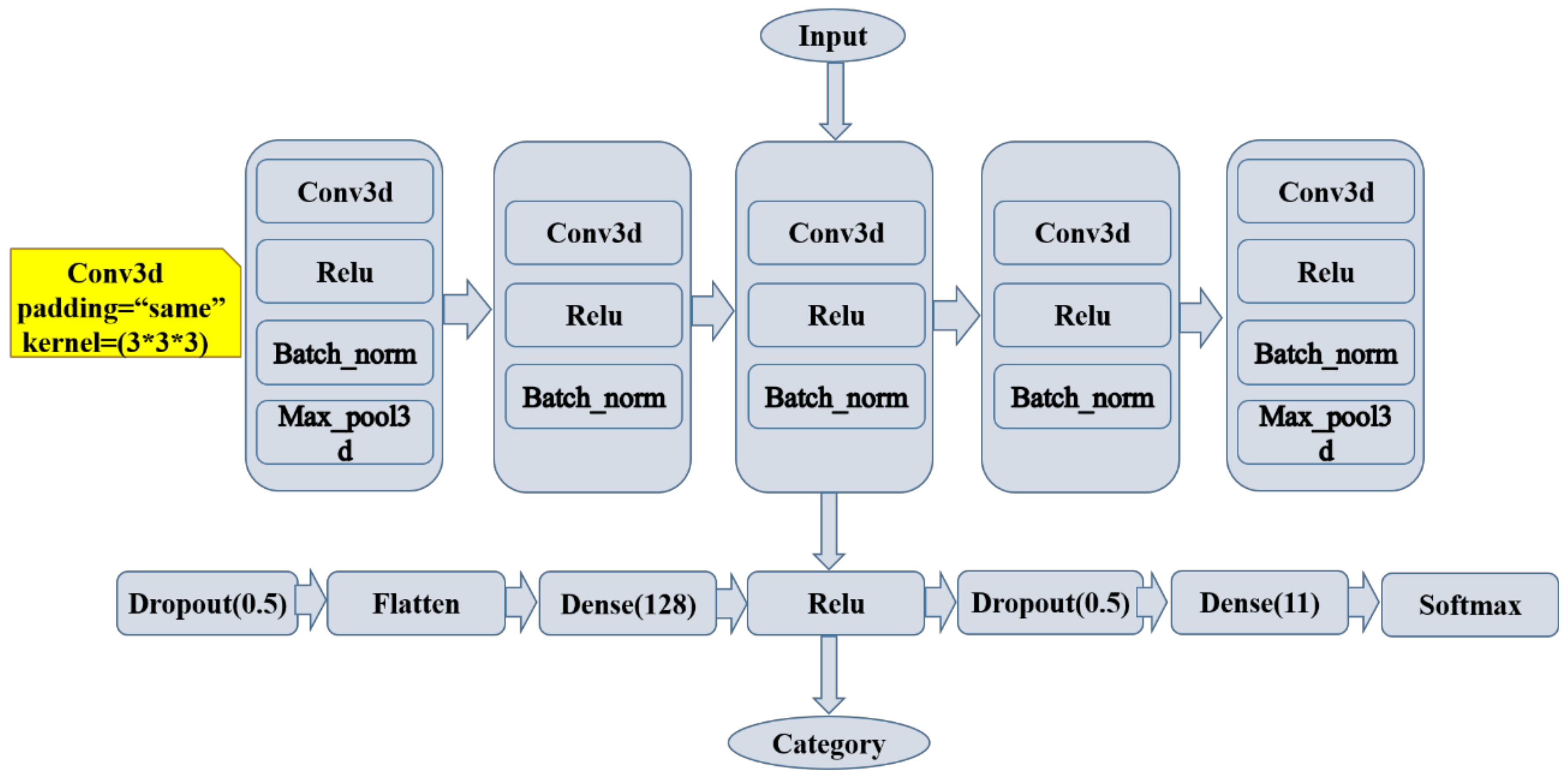
2.6. Three-Dimensional Convolutional Neural Network Construction

In this study, we developed a classification framework based on the 3D-CNN model proposed by Zhang [46] (Figure 6). Five convolutional structures were considered, each of which includes a convolutional layer (Conv3d, padding = “same,” kernel = 3 × 3 × 3), nonlinear activation function (Relu), and batch normalization layer (Batch_norm). The first and last convolution structures set a maximum pooling layer (Max_pool3d), which was used to rapidly reduce the data dimension. Subsequently, we flattened the feature output by the last 3D convolutional layer and transformed the 3D feature cube into features with dimensions of 1 × 128 through the first hidden layer (Dense). These feature vectors passed the Relu linear activation function and entered the second hidden layer (Dense). Moreover, they obtained the features whose dimensions are consistent with the number of categories (11). We used the Softmax activation function to calculate the probability of belonging to each category as the basis for classification. Additionally, to avoid model overfitting, the last convolution structure dropout was added after the output of the first hidden layer and before the second hidden layer, and the Keep_prob was set to 0.7.

Table 2. Three-dimensional convolutional neural network (3D-CNN) model structure.

Layer	Output Shape (Height, Width, Depth, Numbers of Feature Map)	Parameters Number
Conv3d_1	(27, 27, 5, 4)	112
Batch_norm_1	(27, 27, 5, 4)	16
Max_pool3d_1	(9, 9, 2, 4)	0
Conv3d_2	(9, 9, 2, 8)	872
Batch_norm_2	(9, 9, 2, 8)	32
Conv3d_3	(9, 9, 2, 16)	3472
Batch_norm_3	(9, 9, 2, 16)	64
Conv3d_4	(9, 9, 2, 32)	13856
Batch_norm_4	(9, 9, 2, 32)	128
Conv3d_5	(9, 9, 2, 64)	55360
Batch_norm_5	(9, 9, 2, 64)	256
Max_pool3d_2	(3, 3, 1, 64)	0
Dropout_1	(3, 3, 1, 64)	0
Flatten	(576)	0
Dense_1	(128)	73856
Dropout_2	(128)	0
Dense_2	(11)	1419
Total parameters: 149,443
Trainable parameters: 149,195
Non-trainable parameters: 248

presents the output dimensions and training parameters of each model layer.

2.7. Experiments Design

Four experiments were designed to verify the classification performance of the IPrNet in the small-sample dataset and to verify the generalization ability of the network using different window sizes and dimensionality reduction methods. Additionally, 3D-CNN was used to classify tree species to verify whether the IPrNet is advantageous in the classification of small-sample tree species.

(1)

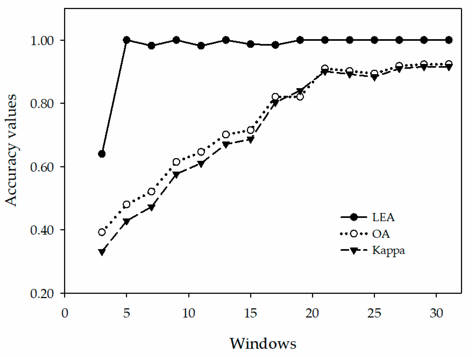
Experiment A: Classification accuracy of the PrNet using different sample windows.

The HSI_PCA was sampled using different window sizes, after which it was sent to the PrNet for classification. To determine whether the PrNet had overfitting before the improvement, this experiment used the unimproved PrNet for classification. The window size started from 3 pixels, increased in steps of 2 pixels, and was set according to the rules of 3 × 3, 5 × 5, 7 × 7, etc., until the cut sample exceeded the study area. Then, the classification accuracy of samples in different windows were compared to find the optimal window. Moreover, if there was a significant difference between the training accuracy (LEA) and the test accuracy (OA, Kappa), it indicates that the network had obvious overfitting.

(2)

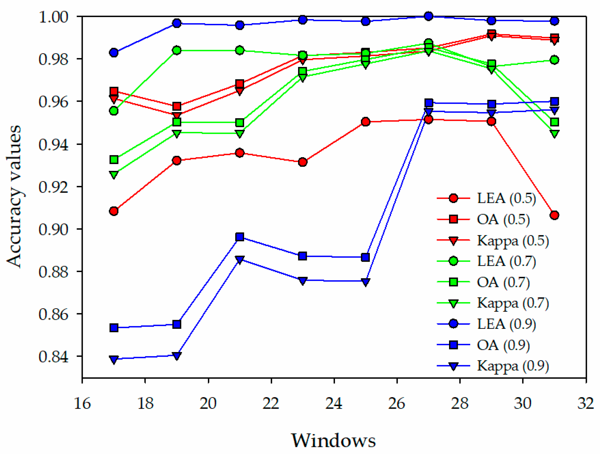
Experiment B: Classification accuracy of the IPrNet using different Keep_prob values.

The HSI_PCA was used as the data source, using IPrNet for classification. The regularization coefficient was set to 0.001, and Keep_prob was set to 0.5, 0.7, and 0.9. The sample window is defined as the window with the highest classification accuracy in experiment A. The experimental results were compared to find the optimal Keep_prob values.

(3)

Experiment C: Classification accuracy of the IPrNet using different data sources.

The HSI, HSI_PCA, and HSI_RF was used as different data sources. The sample window and Keep_prob were set according to the result with the highest classification accuracy in experiment B. Subsequently, we compared the classification accuracy and the network operation efficiency of the IPrNet for different data sources.

(4)

Experiment D: Classification accuracy of the 3D-CNN under the same conditions as Experiment C.

Taking the best sample window of experiment A, the best Keep_prob values of experiment B, and the best data source of experiment C as the experimental conditions, and using 3D-CNN for classification, we compared the classification results of 3D-CNN and IPrNet to verify whether IPrNet had advantages in the classification of small-sample sets.

The increase in the number of network training iterations did not improve the test accuracy of the model. Therefore, the initial number of epochs/iterations was 20/50, and the iterations increased in steps of 50. The optimal number of iterations was tested in turn as a basis for terminating model training.

3. Classification Process and Results

3.1. Classification Using the Prototypical Network

Using the HSI_PCA (914 × 1056 × 5) as the data source, the sample data of different window sizes (3 × 3, 5 × 5, 7 × 7, etc.) were cropped, as the input data of the PrNet. In each class of the training set, five samples were randomly selected as the support set and query to train the model. After adjusting the number of iterations (epochs/iterations), a training accuracy as close to 1 as possible was achieved, to best fit the training samples and to record the training time and network training accuracy (LEA). In each class of the test set, five samples were randomly selected as the query set, and the average test accuracy (OA, Kappa) of the iterative test results were calculated. The results are summarized in

Table 3. Classification accuracy of the prototypical networks (PrNet) in different windows.

Index	3 × 3	5 × 5	7 × 7	9 × 9	11 × 11	13 × 13	15 × 15	17 × 17	19 × 19	21 × 21	23 × 23	25 × 25	27 × 27	29 × 29	31 × 31
Epochs/Iterations	20/500	20/100	20/100	20/100	20/100	20/100	20/100	20/100	20/100	20/100	20/100	20/100	20/100	20/100	20/100
LEA	0.6402	1.0000	0.9822	1.0000	0.9818	1.0000	0.9867	0.9846	1.0000	1.0000	1.0000	1.0000	1.0000	1.0000	1.0000
OA (%)	39.22	48.02	52.04	61.46	64.61	70.10	71.52	82.08	85.50	91.01	90.22	89.42	91.85	92.35	92.40
Kappa	0.3315	0.4282	0.4723	0.5761	0.6107	0.6710	0.6868	0.8028	0.8404	0.9011	0.8924	0.8836	0.9103	0.9159	0.9163
Training Times (S)	68	43	57	122	159	247	314	447	626	732	872	1091	1252	1480	1708

.

For the 3 × 3 window, 20/500 iterations produced the highest classification accuracy. For the 7 × 7–31 × 31 windows, 20/100 iterations produced the highest classification accuracy. To compare the trend of classification accuracy of PrNets for different sample windows, the training accuracy and test accuracy of the model in Table 3 are represented using a line chart (Figure 7). It was evident that as the input data window increased, the test accuracy (OA, Kappa) had three stages: the 3 × 3–21 × 21 windows were the first increase stage, 23 × 23–25 × 25 windows were the declining stage, 27 × 27–31 × 31 windows were the second increase stage. The second increase stage had a moderate trend than the first increase stage. The 31 × 31 window exhibited the maximum accuracy, and the training time increased (Table 3). If the size of the sample windows is increased, the intersection between adjacent samples will also increase, causing the samples near the edge of the image to exceed the boundary that cannot be cropped. Therefore, the maximum setting of the sample window was 31 × 31.

Except for the 3 × 3 window, the training accuracy (LEA) of the PrNet for the remaining windows was close to 1 (Figure 7). However, the difference between the test accuracy and the training accuracy was significant, which indicates overfitting.

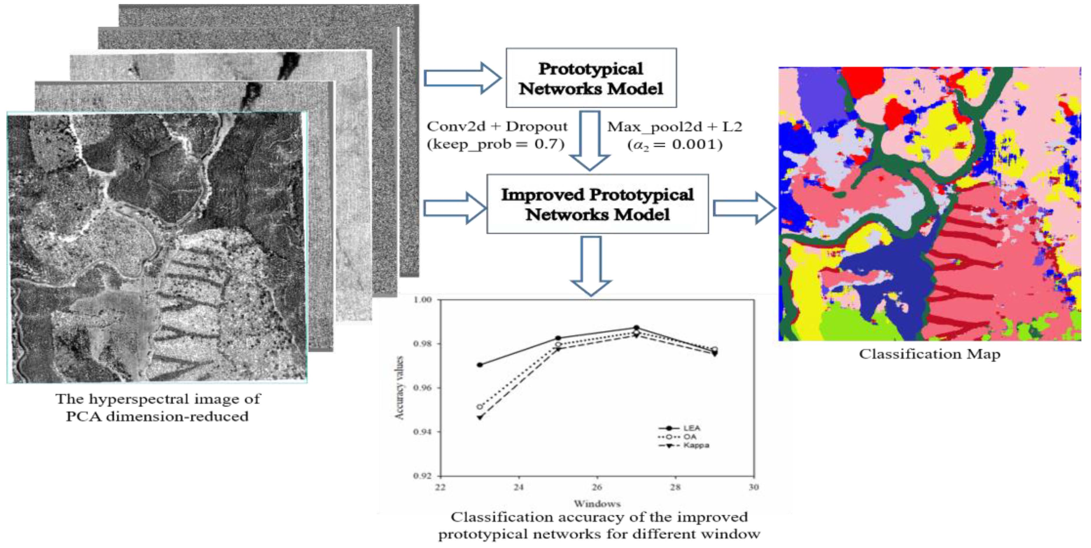
3.2. Classification Using the Improved Prototypical Network

For the sample window of 17 × 17–31 × 31, both the training and test accuracy of the PrNet were relatively high (Figure 7, Table 3). Therefore, these sample windows were selected in experiment B to perform the IPrNet. The classification accuracy is summarized in

Table 4. Classification accuracy of the improved prototypical network (IPrNet) with different Keep_prob.

Index	17 × 17			19 × 19			21 × 21			23 × 23
Dropout	0.5	0.7	0.9	0.5	0.7	0.9	0.5	0.7	0.9	0.5	0.7	0.9
Epochs/Iterations	20/500	20/150	20/100	20/500	20/150	20/100	20/500	20/150	20/100	20/500	20/150	20/100
LEA	0.9084	0.9555	0.9829	0.9322	0.9840	0.9967	0.9358	0.9840	0.9958	0.9314	0.9816	0.9984
OA (%)	96.49	93.26	85.35	95.77	95.02	85.51	96.83	95.01	89.62	98.15	97.41	88.72
Kappa	0.9614	0.9259	0.8388	0.9535	0.9452	0.8406	0.9652	0.9451	0.8858	0.9796	0.9715	0.8759
Training Times (S)	2245	684	463	2961	887	593	3821	1132	753	4351	1299	874
Index	25 × 25			27 × 27			29 × 29			31 × 31
Dropout	0.5	0.7	0.9	0.5	0.7	0.9	0.5	0.7	0.9	0.5	0.7	0.9
Epochs/Iterations	20/500	20/100	20/100	20/500	20/100	20/100	20/500	20/100	20/100	20/500	20/100	20/100
LEA	0.9504	0.9826	0.9976	0.9515	0.9874	1.0000	0.9506	0.9764	0.9980	0.9065	0.9795	0.9978
OA (%)	98.30	97.97	88.67	98.52	98.53	95.94	99.17	97.76	95.88	98.98	95.02	96.01
Kappa	0.9813	0.9777	0.8754	0.9837	0.9838	0.9553	0.9909	0.9754	0.9547	0.9888	0.9452	0.9561
Training Times (S)	5403	1122	1091	6458	1290	1275	7190	1449	1443	9565	1676	1669

. After testing, when the Keep_prob was 0.5, the number of iterations with the highest classification accuracy was 20/500. When Keep_prob was 0.7, the number of iterations with the highest classification accuracy was 20/150 in 17 × 17–23 × 23 sample windows, and the number of iterations with the highest classification accuracy was 20/100 in 25 × 25–31 × 31 sample windows. Finally, when Keep_prob was 0.9, the number of iterations with the highest classification accuracy was 20/100.

To compare the trend of changes in the classification accuracy with respect to different windows and different Keep_prob values, the network training accuracy and test accuracy in Table 4 are represented using a line chart (Figure 8). Overall, the difference between the training accuracy and test accuracy of the IPrNet was smaller than that in the case of experiment A. This indicates that the IPrNet proposed in this study could effectively address the overfitting problem. When Keep_prob was 0.5, the difference between the training accuracy (LEA) and the test accuracy (OA, Kappa) of the network was relatively large, and the run-time of the network was the longest. When Keep_prob was 0.7, a certain difference existed between the training accuracy and the test accuracy of the network in the sample windows of 17 × 17–21 × 21 and 31 × 31. In the sample windows of 23 × 23–29 × 29, the training accuracy and the test accuracy of the network were nearly identical, there was no overfitting in the network. In the sample windows of 23 × 23–27 × 27, the network classification accuracy was in the rising stage, and in the 29 × 29 sample window, the network classification accuracy was reduced. When Keep_prob was 0.9, the difference between the training accuracy and the test accuracy of the network was the largest, and the overfitting problem was not sufficiently addressed.

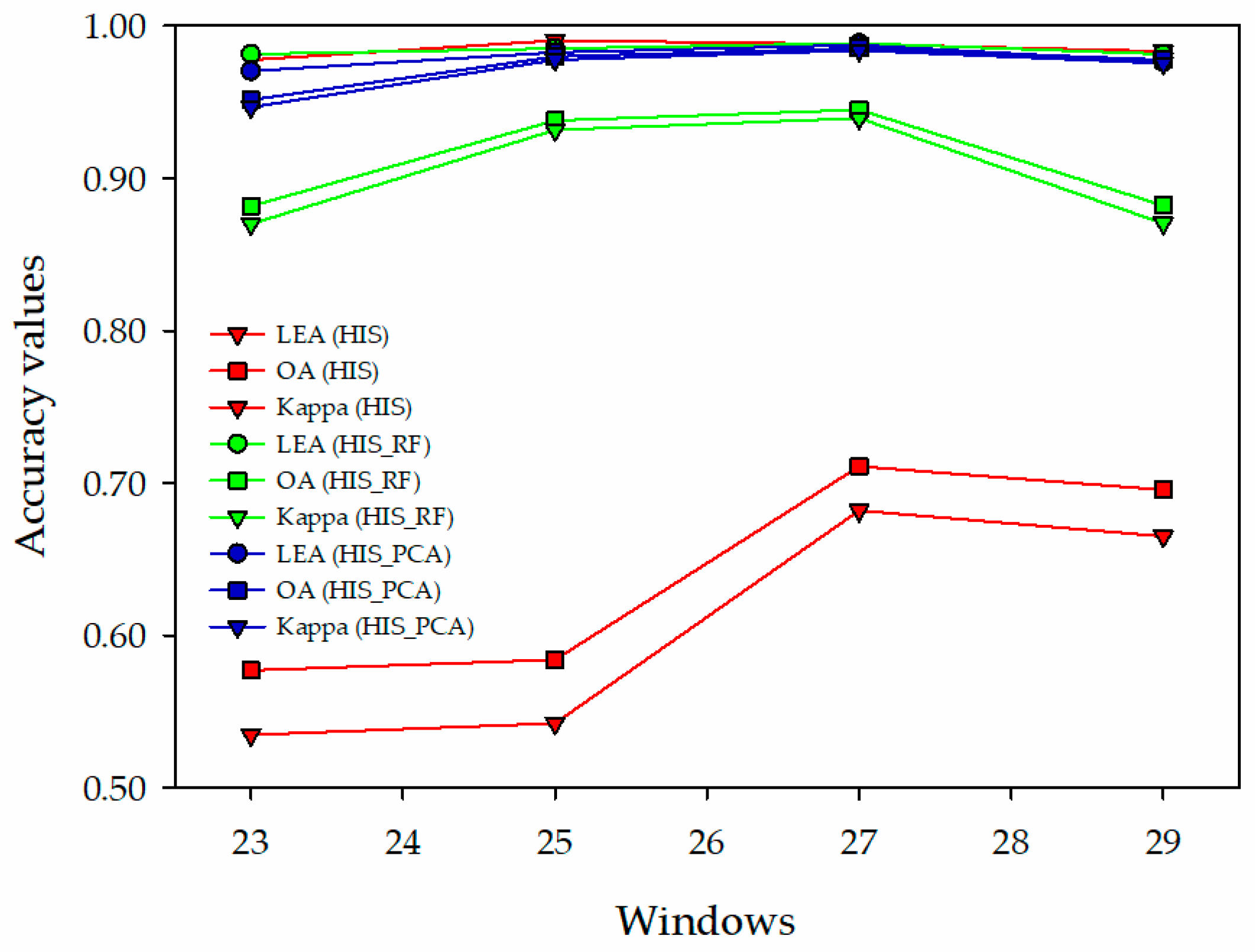
3.3. Classification Using the Improved Prototypical Network with Different Data Sources

When Keep_prob was 0.7 and the sample windows were 23 × 23–29 × 29, the IPrNet had no overfitting (Figure 8, Table 4). Therefore, IPrNet was used to perform experiment C under the following test conditions: the HSI (914 × 1056 × 125), HSI_RF (914 × 1056 × 8, RF), and the HSI_PCA (914 × 1056 × 5, PCA) were used as the data source, Keep_prob was set to 0.7, the sample windows were 23 × 23–29 × 29, and the number of iterations was 20/100. The producer accuracy of each category was calculated, that is, the probability of correctly classifying a category from the total number of samples of that category. The results are summarized in

Table 5. Classification accuracy of the improved prototypical network (IPrNet) with different data source.

Index/Categories	23 × 23			25 × 25			27 × 27			29 × 29
	HSI	HSI_RF	HSI_PCA	HSI	HSI_RF	HSI_PCA	HSI	HSI_RF	HSI_PCA	HSI	HSI_RF	HSI_PCA
Epochs/iterations	20/100	20/100	20/100	20/100	20/100	20/100	20/100	20/100	20/100	20/100	20/100	20/100
LEA	0.9776	0.9815	0.9704	0.9904	0.9851	0.9826	0.9880	0.9886	0.9874	0.9833	0.9815	0.9764
OA (%)	57.70	88.17	95.14	58.39	93.78	97.97	71.08	94.49	98.53	69.54	88.22	97.76
Kappa	0.5347	0.8699	0.9466	0.5423	0.9316	0.9777	0.6819	0.9394	0.9838	0.6650	0.8704	0.9754
Training Times (S)	1806	906	893	2057	1124	1122	2406	1308	1290	2774	1536	1449
C. lanceolata	0.5034	0.7624	0.9590	0.5306	0.9166	1.0000	0.4536	0.9186	1.0000	0.6470	0.9554	0.9976
P. elliottii	0.1852	0.6916	0.8210	0.3958	0.7810	0.8818	0.5558	0.7862	0.9374	0.5092	0.6754	0.9440
P. massoniana	0.4894	0.9342	0.9998	0.6598	0.9996	0.9970	0.8812	0.9962	1.0000	0.4814	0.6630	1.0000
E. urophylla	0.4980	0.7896	0.9258	0.5612	0.9776	0.9394	0.4604	0.8782	1.0000	0.8630	0.9554	0.9954
E. grandis	0.7660	0.9970	0.9238	0.9336	0.8920	0.9968	0.5574	0.9524	1.0000	0.9856	0.9464	0.9282
C. hystrix	0.5286	0.9590	0.9382	0.5912	0.8472	0.9552	0.9314	0.9330	0.9818	0.7570	0.9468	0.9922
A. melanoxylon	0.4792	0.8426	1.0000	0.5962	0.9962	0.9998	0.7338	0.9998	0.9992	0.4918	1.0000	1.0000
M. laosensis	0.3608	0.7292	0.9024	0.2752	0.9500	0.9568	0.4936	0.8870	0.9950	0.6176	0.6740	0.9696
Soft broadleaf	0.6344	0.9934	0.9958	0.7674	0.9558	0.9996	0.8376	0.9948	0.9602	0.7192	0.8874	1.0000
Cutting site	0.9450	1.0000	1.0000	0.3530	1.0000	1.0000	0.9610	1.0000	1.0000	0.8664	1.0000	1.0000
Road	0.9568	1.0000	1.0000	0.7592	1.0000	1.0000	0.9532	1.0000	1.0000	0.7114	1.0000	1.0000

. The network training accuracy and test accuracy in Table 5 are represented using a line chart (Figure 9) to compare the classification accuracy trends for different data sources. The OA (57.70–71.08%) and Kappa (0.5347–0.6819) of the HSI were low, and the running time of the network was the longest (1806–2774’s, Table 5). Furthermore, the OA (88.17–94.49%) and Kappa (0.8699–0.9394) were relatively low for the HSI_RF, and the running time was relatively short (906–1536 s). Notably, the highest OA (95.14–98.53%) and Kappa (0.9466–0.9838) and the shortest running time (893–1449 s) were of the HSI_PCA. The test accuracy of different data sources increased in the 23 × 23–27 × 27 sample windows and decreased in the 29 × 29 sample window.

The producer accuracy of each tree species is presented in Table 5. The accuracy of C. lanceolata (CL) and P. massoniana (PM) were higher, and the accuracy of P. elliottii (PE) was lower in coniferous. The conifers were suitable for classification using the HSI_PCA. Among them, the accuracy of C. lanceolata (CL) in the 25 × 25 and 27 × 27 sample windows reached 100%, and the accuracy of P. massoniana (PM) in the 27 × 27 and 29 × 29 sample windows reached 100%. In the broadleaf species, E. urophylla (EU), E. grandis (EG), A. melanoxylon (AM), and soft broadleaf (SB) had relatively high classification accuracy, and C. hystrix (CH) and M. laosensis (ML) had relatively low classification accuracy. Broadleaf trees were also suitable for classification using the HSI_PCA. Among them, the accuracy of E. urophylla (EU) and E. grandis (EG) in the 27 × 27 sample windows reached 100%. Additionally, the accuracy of soft broadleaf (SB) in the 29 × 29 sample windows reached 100%.

3.4. Comparison to 3D-CNN

The IPrNet had the highest classification accuracy under the following conditions: the PCA dimension-reduced HSIs were used as the data source, the sample window was 27 × 27, Keep_prob was 0.7, and the number of iterations was 20/100 (Figure 9, Table 5). Therefore, under the conditions of the same data source, network parameters, and sample windows, 3D-CNN was used to classify tree species to test the difference between the classification performance of the IPrNet and 3D-CNN under small-sample conditions.

Table 6. Classification accuracy of the improved prototypical network (IPrNet) and the three-dimensional convolutional neural network (3D-CNN) model.

Index/Categories	IPrNet	3D-CNN
LEA	0.9874	0.8920
OA (%)	98.53	87.50
Kappa	0.9838	0.8625
Training Times (S)	1290	4986
C. lanceolata	1.0000	0.8214
P. elliottii	0.9374	0.8889
P. massoniana	1.0000	0.7586
E. urophylla	1.0000	0.7407
E. grandis	1.0000	0.8148
C. hystrix	0.9818	0.9167
A. melanoxylon	0.9992	0.8333
M. laosensis	0.9950	0.9375
Soft broadleaf	0.9602	1.0000
Cutting site	1.0000	1.0000
Road	1.0000	1.0000

presents the classification results. Compared with the classification results of the IPrNet, the network training accuracy (LEA) and test accuracy (OA, Kappa) of the 3D-CNN model were relatively low, and the network training time was long. In the classification results of each tree species, only the classification accuracy of C. hystrix (CH), M. laosensis (ML), and soft broadleaf (SB) was >90%, whereas the classification accuracy of the other tree species was relatively low. Therefore, in the small-sample tree species classification application, the IPrNet had a higher classification performance, and the network training time significantly shortened.

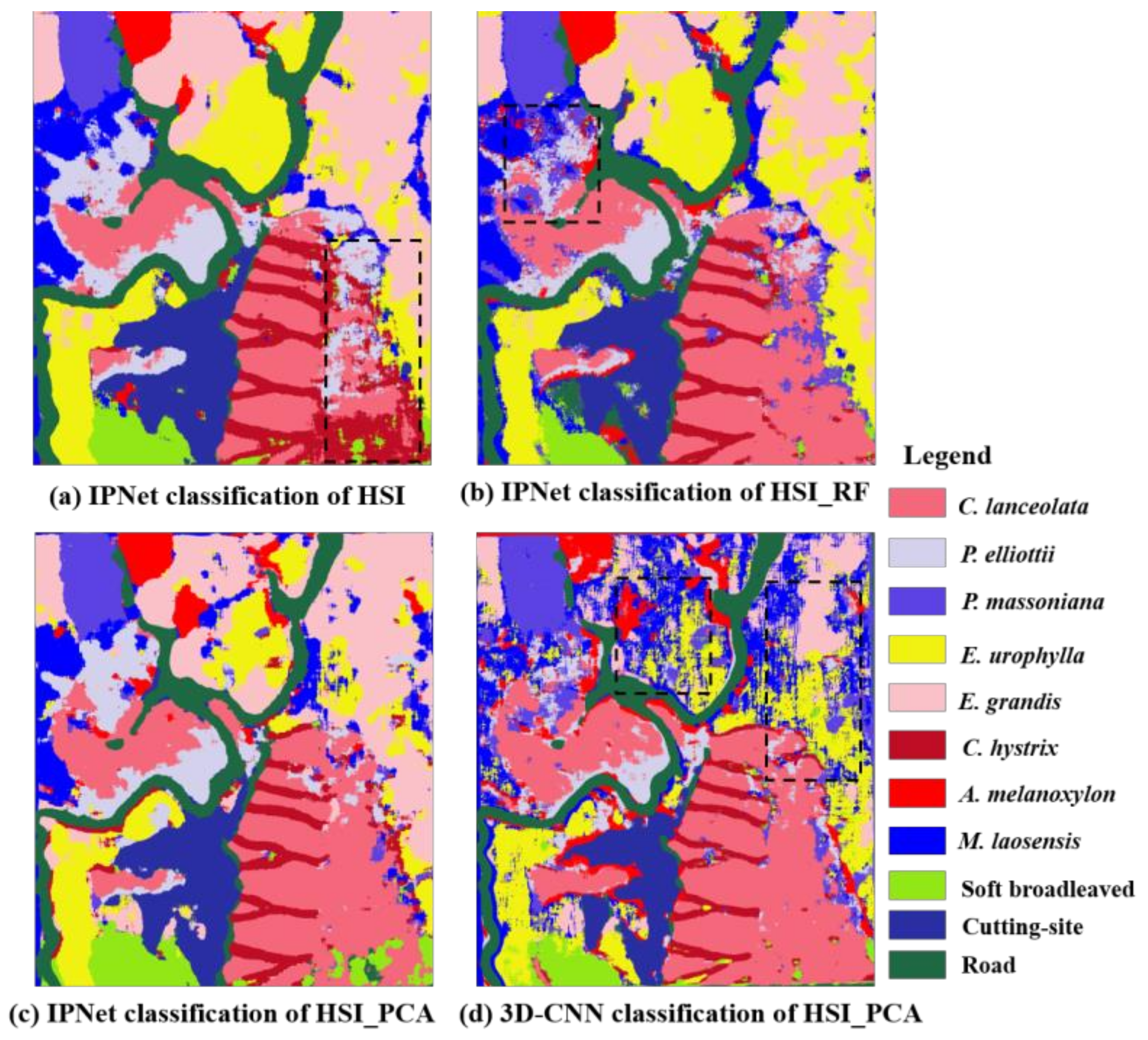
3.5. Classification Results Map

In this study, we used the pixel-by-pixel method as the sample center point to obtain the prediction result of the optimal window (27 × 27) and generated a classification map (Figure 10). In the IPrNet classification map of HSI (a), the boundary of the mixed area of C. lanceolata (CL), P. elliottii (PE), and C. hystrix (CH) is unclear. Additionally, in the IPrNet classification map of HSI_RF (b), the boundary of the mixed area of P. elliottii (PE), P. massoniana (PM), and M. laosensis (ML) is unclear. In the 3D-CNN classification map of HSI_PCA (d), the boundary of each tree species distribution area was not clear, and the classification effect was not ideal. However, the IPrNet classification map of HSI_PCA (c) could clearly distinguish various types of features in the study area, which is of great significance for the management and effective monitoring of forest resources.

4. Discussion

4.1. The Size of the Sample Windows on the Classification of the Prototypical Network

When the PrNet classifies the HSI_PCA, the size of the sample windows had a great influence on the classification accuracy. Employing an appropriate size of the sample windows helped improve the classification performance of the PrNet. However, samples with excessively large windows may cause additional noise [47] and increase the time of network training and the amount of prediction calculations. In this study, the classification accuracy of the PrNet reached a peak for the 21 × 21 sample window, indicating that the 21 × 21 sample window is the optimal window for classification of the PrNet. It had a significant effect on tree crown segmentation and generated appropriate sample data. According to these sample data, the HSI of the study area could be classified with high precision. In the 23 × 23 and 25 × 25 sample windows, the classification accuracy was reduced as a result of the influence of data noise caused by the large size of the sample windows. When the size of the sample windows continued to increase, the classification accuracy of the PrNet slowly increased, which may be because the data noise is masked with an increase in the sample windows. When the size of the sample windows matched the spatial distribution pattern of the forest, the PrNet exhibited higher classification accuracy. This indicates that the size and distribution pattern of the forest stand area had an influence on the selection of windows. In practical applications, the window size should therefore be determined according to the size of the area and the distribution pattern of the forest stand.

The IPrNet proposed in this study could effectively classify tree species of small samples. However, the classification accuracy trend of the IPrNet in different sample windows was changed, and the optimal classification window was 27 × 27. Therefore, changes in the network structure led to inconsistent requirements for the size of the sample windows. The noise in the sample data can be effectively avoided using the optimal window, and higher classification accuracy can thus be achieved [48].

4.2. Different Data Sources on Classification of the Improved Prototypical Network

The IPrNet exhibited different classification accuracies for different data sources. However, the optimal classification sample window was 27 × 27. Since the HSI has many bands with strong correlations, the IPrNet exhibited the longest training time and low classification accuracy for the classification of the HSI. Additionally, the classification accuracy of the IPrNet for E. grandis (EG), C. hystrix (CH), cutting site, and roads were more than 93%. From the classification results (Figure 10), it was evident that the distribution of these categories was relatively concentrated, and the distribution range was more regular, leading to higher classification accuracy.

After RF dimensionality reduction processing, the HSI retained eight bands of high importance. The reduction in data volume reduced the training time of the IPrNet, and the removal of a large amount of redundant information made the test accuracy of the network significant compared to that obtained using the HSI. After PCA dimensionality reduction processing, the HSI retained the first five components, effectively mapping the high-dimensional data to a few low-dimensional vectors containing the main information. When using the IPrNet to classify the data sources of the two dimensionality reduction methods, the PCA dimensionality reduction image had the shortest network training time and the highest test accuracy. This may be caused by the PCA dimensionality reduction method further compressing the HSI. Consequently, the IPrNet exhibited better performance for data classification with simple structures. The IPrNet has relatively low classification accuracy for the coniferous species P. elliottii (PE), the broadleaf species C. hystrix (CH), and M. laosensis (ML). This may be due to the small distribution area of P. elliottii (PE) and M. laosensis (ML), and the fragmented distribution patch; therefore, the classification process is easily affected by other tree species [49]. The C. hystrix (CH) trees are distributed in strips; when the cropping sample window is large, it is easy to crop adjacent tree species as samples, which affects the classification accuracy.

4.3. The Advantage of the Improved Prototypical Network

The IPrNet is a simple and efficient network that has great advantages compared with the 3D-CNN. From the network layer, the 3D-CNN uses Conv3d and Maxpooling3d, and the IPrNet uses Conv2d and Maxpooling2d. Thus, the training weight coefficient of the IPrNet reduces, and the training time. From the network structure, the 3D-CNN uses cross-entropy loss to classify, the IPrNet uses a distance function to calculate the probability of belonging to each category, and the Euclidean distance function satisfies the Bregman divergence, which renders it easier to classify the samples spatially.

The network operation results revealed that the IPrNet obtained the best classification results compared with the 3D-CNN model (Table 6). Training the 3D-CNN model is time consuming, and the classification accuracy is low. The classification results of 3D-CNN were fragmented, the edges were rough, the accuracy was low, and severe mixing occurred between tree species (Figure 10). The IPrNet structure is simple and can achieve high classification accuracy and short training time in the classification of small-samples of tree species. In addition, the IPrNet can extract information at different scales of the image and identify tree species in smaller areas. At the same time, it avoids the gradient degradation problem caused by the deepening of the network layer, to obtain the best classification effect. Thus, IPrNet can be an effective method for the classification of complex tree species in Southern China.

5. Conclusions

In this study, an improved prototypical network (IPrNet) was proposed. It performed better than 3D-CNN in the classification of forest tree species with a small-sample dataset. Comparing with 3D-CNN model, IPrNet training required fewer weight coefficients. Using Bregman divergence as the proximity measurement function, the convergence, and local minimum of the clustering algorithm were the same as the usual K-means. The Euclidean distance function satisfied the Bregman divergence. When the IPrNet is connected with clustering, it is reasonable to use the class means as the prototype for clustering, which made it easier to classify samples in space. The classification of airborne HSIs of nine complex forest tree species, cutting site, and roads in a 74.1 hm² study area required only 1290’s. The OA reached 98.53%, and the Kappa reached 0.9838, which is suitable for regional tree species classification and mapping.

The different window samples were input into the IPrNet for classification, where an optimal classification window existed. The window size should be determined according to the area size and forest stand distribution pattern. Furthermore, the improved method of adding L2 regularization to the convolutional layer and dropout to the maximum pooling layer could effectively address the network overfitting. In actual classification applications, the IPrNet can effectively solve the classification problem of small-sample sets.

The IPrNet classified the tree species of airborne HSIs without dimensionality reduction, the results had a long training time and low test accuracy. After the dimensionality reduction of airborne HSIs, the training time was halved, and the test accuracy was significantly increased. Moreover, the classification accuracy of the HSI_PCA was higher than that of the HSI_RF, and the network training time of the HSI_PCA was shorter than that of the HSI_RF. Thus, using the IPrNet to classify the HSI after PCA dimensionality reduction can achieve desirable classification results.

References

1. Guo, M.; Li, J.; Sheng, C.; Xu, J.; Wu, L. A review of wetland remote sensing. Sensors 2017, 17, 777. [Google Scholar] [CrossRef] [Green Version]
2. Pu, R.; Gong, P.; Heald, R. In situ hyperspectral data analysis for nutrient estimation of giant sequoia. In Proceedings of the IEEE 1999 International Geoscience and Remote Sensing Symposium IGARSS’99, Hamburg, Germany, 28 June–2 July 1999; (Cat. No. 99CH36293). Volume 23, pp. 1827–1850. [Google Scholar] [CrossRef]
3. Liu, L.; Coops, N.; Aven, N.W.; Pang, Y. Mapping urban tree species using integrated airborne hyperspectral and LiDAR remote sensing data. Remote. Sens. Environ. 2017, 200, 170–182. [Google Scholar] [CrossRef]
4. Cao, J.; Leng, W.; Liu, K.; Liu, L.; He, Z.; Zhu, Y. Object-based mangrove species classification using unmanned aerial vehicle hyperspectral images and digital surface models. Remote. Sens. 2018, 10, 89. [Google Scholar] [CrossRef] [Green Version]
5. Zhong, Y.; Cao, Q.; Zhao, J.; Ma, A.; Zhao, B.; Zhang, L. Optimal decision fusion for urban land-use/land-cover classification based on adaptive differential evolution using hyperspectral and LiDAR data. Remote. Sens. 2017, 9, 868. [Google Scholar] [CrossRef] [Green Version]
6. Berhane, T.M.; Lane, C.R.; Wu, Q.; Autrey, B.C.; Anenkhonov, O.A.; Chepinoga, V.V.; Liu, H. Decision-tree, rule-based, and random forest classification of high-resolution multispectral imagery for wetland mapping and inventory. Remote. Sens. 2018, 10, 580. [Google Scholar] [CrossRef] [PubMed] [Green Version]
7. Hughes, G. On the mean accuracy of statistical pattern recognizers. IEEE Trans. Inf. Theory 1968, 14, 55–63. [Google Scholar] [CrossRef] [Green Version]
8. Chen, C.; Jiang, F.; Yang, C.; Rho, S.; Shen, W.; Liu, S.; Liu, Z. Hyperspectral classification based on spectral–spatial convolutional neural networks. Eng. Appl. Artif. Intell. 2018, 68, 165–171. [Google Scholar] [CrossRef]
9. Harsanyi, J.; Chang, C.-I. Hyperspectral image classification and dimensionality reduction: An orthogonal subspace projection approach. IEEE Trans. Geosci. Remote. Sens. 1994, 32, 779–785. [Google Scholar] [CrossRef] [Green Version]
10. Sagan, V.; Asari, V.K.; Sagan, V. Progressively Expanded Neural Network (PEN Net) for hyperspectral image classification: A new neural network paradigm for remote sensing image analysis. ISPRS J. Photogramm. Remote. Sens. 2018, 146, 161–181. [Google Scholar] [CrossRef]
11. Chang, C.-I.; Du, Q.; Sun, T.-L.; Althouse, M.L.G. A joint band prioritization and band-decorrelation approach to band selection for hyperspectral image classification. IEEE Trans. Geosci. Remote. Sens. 1999, 37, 2631–2641. [Google Scholar] [CrossRef] [Green Version]
12. Shi, Y.; Wang, T.; Wang, T.; Holzwarth, S.; Heiden, U.; Pinnel, N.; Zhu, X.; Heurich, M. Tree species classification using plant functional traits from LiDAR and hyperspectral data. Int. J. Appl. Earth Obs. Geoinf. 2018, 73, 207–219. [Google Scholar] [CrossRef]
13. Ma, L.; Li, M.; Ma, X.; Cheng, L.; Du, P.; Liu, Y. A review of supervised object-based land-cover image classification. ISPRS J. Photogramm. Remote. Sens. 2017, 130, 277–293. [Google Scholar] [CrossRef]
14. Wu, Y.; Zhang, X. Object-based tree species classification using airborne hyperspectral images and LiDAR data. Forests 2019, 11, 32. [Google Scholar] [CrossRef] [Green Version]
15. Zhao, W.; Du, S. Learning multiscale and deep representations for classifying remotely sensed imagery. ISPRS J. Photogramm. Remote. Sens. 2016, 113, 155–165. [Google Scholar] [CrossRef]
16. Ghosh, A.; Joshi, P.K. A comparison of selected classification algorithms for mapping bamboo patches in lower Gangetic plains using very high resolution WorldView 2 imagery. Int. J. Appl. Earth Obs. Geoinf. 2014, 26, 298–311. [Google Scholar] [CrossRef]
17. Benediktsson, J.A.; Swain, P.H.; Ersoy, O.K. Conjugate-gradient neural networks in classification of multisource and very-high-dimensional remote sensing data. Int. J. Remote. Sens. 1993, 14, 2883–2903. [Google Scholar] [CrossRef]
18. Keshk, H.; Yin, X.-C. Classification of EgyptSat-1 images using deep learning methods. Int. J. Sensors, Wirel. Commun. Control. 2020, 10, 37–46. [Google Scholar] [CrossRef]
19. Lecun, Y.; Bengio, Y.; Hinton, G. Deep learning. Nature 2015, 521, 436–444. [Google Scholar] [CrossRef]
20. Pan, B.; Shi, Z.; Xu, X. MugNet: Deep learning for hyperspectral image classification using limited samples. ISPRS J. Photogramm. Remote. Sens. 2018, 145, 108–119. [Google Scholar] [CrossRef]
21. Guo, Y.; Han, S.; Cao, H.; Zhang, Y.; Wang, Q. Guided filter based deep recurrent neural networks for hyperspectral image classification. Procedia Comput. Sci. 2018, 129, 219–223. [Google Scholar] [CrossRef]
22. Hartling, S.; Sagan, V.; Sidike, P.; Maimaitijiang, M. Urban tree species classification using a WorldView-2/3 and LiDAR data fusion approach and deep learning. Sensors 2019, 19, 1284. [Google Scholar] [CrossRef] [PubMed] [Green Version]
23. Han, M.; Cong, R.; Li, X.; Fu, H.; Lei, J. Joint spatial-spectral hyperspectral image classification based on convolutional neural network. Pattern Recognit. Lett. 2020, 130, 38–45. [Google Scholar] [CrossRef]
24. Ashiquzzaman, A.; Tushar, A.K.; Islam, R.; Shon, D.; Im, K.; Park, J.-H.; Lim, D.-S.; Kim, J. Reduction of overfitting in diabetes prediction using deep learning neural network. In IT Convergence and Security 2017; Springer: Singapore, 2018; Volume 449, pp. 35–43. [Google Scholar] [CrossRef] [Green Version]
25. Hinton, G.; Deng, L.; Yu, D.; Dahl, G.E.; Mohamed, A.-R.; Jaitly, N.; Senior, A.; Vanhoucke, V.; Nguyen, P.; Sainath, T.N.; et al. Deep neural networks for acoustic modeling in speech recognition: The shared views of four research groups. IEEE Signal. Process. Mag. 2012, 29, 82–97. [Google Scholar] [CrossRef]
26. Tong, Q.X.; Xue, Y.Q.; Zhang, L.F. Progress in hyperspectral remote sensing science and technology in China over the past threedecades. IEEE J. Stars. 2014, 7, 70–91. [Google Scholar]
27. Li, Y.; Li, Q.; Liu, Y.; Xie, W. A spatial-spectral SIFT for hyperspectral image matching and classification. Pattern Recognit. Lett. 2019, 127, 18–26. [Google Scholar] [CrossRef]
28. Li, S.; Song, W.; Fang, L.; Chen, Y.; Ghamisi, P.; Benediktsson, J.A. Deep learning for hyperspectral image classification: An overview. IEEE Trans. Geosci. Remote. Sens. 2019, 57, 6690–6709. [Google Scholar] [CrossRef] [Green Version]
29. Pan, B.; Shi, Z.; Xu, X. R-VCANet: A new deep-learning-based hyperspectral image classification method. IEEE J. Sel. Top. Appl. Earth Obs. Remote. Sens. 2017, 10, 1975–1986. [Google Scholar] [CrossRef]
30. Xu, Y.; Du, B.; Zhang, F.; Zhang, L. Hyperspectral image classification via a random patches network. ISPRS J. Photogramm. Remote. Sens. 2018, 142, 344–357. [Google Scholar] [CrossRef]
31. Fricker, G.A.; Ventura, J.D.; Wolf, J.A.; North, M.P.; Davis, F.W.; Franklin, J. A Convolutional neural network classifier identifies tree species in mixed-conifer forest from hyperspectral imagery. Remote. Sens. 2019, 11, 2326. [Google Scholar] [CrossRef] [Green Version]
32. Krizhevsky, A.; Sutskever, I.; Hinton, G.E. ImageNet classification with deep convolutional neural networks. In Advances in Neural Information Processing Systems 25; Pereira, F., Burges, C.J.C., Bottou, L., Weinberger, K.Q., Eds.; Curran Associates, Inc.: Red Hook, NY, USA, 2012; pp. 1097–1105. [Google Scholar]
33. Simonyan, K.; Zisserman, A. Very deep convolutional networks for large-scale image recognition. arXiv 2014, arXiv:1409.1556. [Google Scholar]
34. Howard, A.G.; Zhu, M.; Chen, B.; Kalenichenko, D.; Wang, W.; Weyand, T.; Andreetto, M.; Adam, H. MobileNets: Efficient convolutional neural networks for mobile vision applications. arXiv 2017, arXiv:1704.04861. [Google Scholar]
35. Sandler, M.; Howard, A.; Zhu, M.; Zhmoginov, A.; Chen, L.-C. MobileNetV2: Inverted residuals and linear bottlenecks. In Proceedings of the 2018 IEEE/CVF Conference on Computer Vision and Pattern Recognition, Salt Lake City, UT, USA, 18–23 June 2018; pp. 4510–4520. [Google Scholar]
36. Paoletti, M.; Haut, J.; Plaza, J.; Plaza, A. A new deep convolutional neural network for fast hyperspectral image classification. ISPRS J. Photogramm. Remote. Sens. 2018, 145, 120–147. [Google Scholar] [CrossRef]
37. Audebert, N.; Le Saux, B.; Lefèvre, S. Deep learning for classification of hyperspectral data: A comparative review. IEEE Geosci. Remote. Sens. Mag. 2019, 7, 159–173. [Google Scholar] [CrossRef] [Green Version]
38. Vilalta, R.; Drissi, Y. A perspective view and survey of meta-learning. Artif. Intell. Rev. 2002, 18, 77–95. [Google Scholar] [CrossRef]
39. Bernhard, P.; Hilan, B.; Christophe, G.G. Meta-learning by landmarking various learning algorithms. In Proceedings of the 17th International Conference on Machine Learning, Stanford University, Stanford, CA, USA, 29 June–2 July 2000. [Google Scholar]
40. Vinyals, O.; Blundell, C.; Lillicrap, T.; Kavukcuoglu, K.; Wierstra, D. Matching Networks for One Shot Learning. Proceedings of Advances in Neural Information Processing Systems (NIPS 2016), Barcelona, Spain, 5–10 December 2016; pp. 3630–3638. [Google Scholar]
41. Fort, S. Gaussian Prototypical Networks for Few-Shot Learning on Omniglot. Proceedings of Bayesian Deep Learning NIPS 2017 Workshop, Long Beach, CA, USA, 9 December 2017. [Google Scholar]
42. Snell, J.; Swersky, K.; Zemel, R.S. Prototypical Networks for Few-shot Learning. Proceeding of Advances in Neural Information Processing Systems, NIPS 2017, Long Beach, CA, USA, 4–9 December 2017; pp. 4077–4087. [Google Scholar]
43. Zhang, L.; Lu, G. Study on the biomass of chinese fir plantation in state-owned Gao Feng Forest Farm of Guangxi. For. Sci. Technol. Rep. 2019, 51, 43–47. [Google Scholar]
44. Hao, J.; Yang, W.; Li, Y.; Hao, J. Atmospheric correction of multi-spectral imagery ASTER. Remote Sens. 2008, 1, 7–81. [Google Scholar]
45. Zhang, N.; Zhang, X.; Yang, G.; Zhu, C.; Huo, L.; Feng, H. Assessment of defoliation during the Dendrolimus tabulaeformis Tsai et Liu disaster outbreak using UAV-based hyperspectral images. Remote. Sens. Environ. 2018, 217, 323–339. [Google Scholar] [CrossRef]
46. Zhang, B.; Zhao, L.; Zhang, X. Three-dimensional convolutional neural network model for tree species classification using airborne hyperspectral images. Remote. Sens. Environ. 2020, 247, 111938. [Google Scholar] [CrossRef]
47. Cao, K.; Zhang, X. An improved res-UNet model for tree species classification using airborne high-resolution images. Remote. Sens. 2020, 12, 1128. [Google Scholar] [CrossRef] [Green Version]
48. Mahdianpari, M.; Salehi, B.; Rezaee, M.; Mohammadimanesh, F.; Zhang, Y. Very deep convolutional neural networks for complex land cover mapping using multispectral remote sensing imagery. Remote. Sens. 2018, 10, 1119. [Google Scholar] [CrossRef] [Green Version]
49. Yu, S.; Jia, S.; Xu, C. Convolutional neural networks for hyperspectral image classification. Neurocomputing 2017, 219, 88–98. [Google Scholar] [CrossRef]
Figure 1. Location of the study area. (a) Vector map of Guangxi Prefecture-level city; (b) digital orthophoto map (DOM) of Jiepai Forest Farm; (c) hyperspectral images of the study area (false color composite (FCC); R, band 53; G, band 34; B, band 16); and (d) distribution of sample points.
Remotesensing 12 03839 g001
Figure 2. Sample data construction process.
Remotesensing 12 03839 g002
Figure 3. Schematic of the prototypical network (PrNet).
Remotesensing 12 03839 g003
Figure 4. Loss calculation algorithm for prototype network (PrNet) training.
Remotesensing 12 03839 g004
Figure 5. Tree species classification framework based on the improved prototypical network (IPrNet).
Remotesensing 12 03839 g005
Figure 6. Tree species classification framework based on the three-dimensional convolutional neural network (3D-CNN) model.
Remotesensing 12 03839 g006
Figure 7. Classification accuracy of the prototypical networks (PrNets) for different windows.
Remotesensing 12 03839 g007
Figure 8. Classification accuracy of the improved prototypical network (IPrNet).
Remotesensing 12 03839 g008
Figure 9. Trend of classification accuracy of the improved prototypical network (IPrNet) with different data sources.
Remotesensing 12 03839 g009
Figure 10. Classification map of the improved prototypical network (IPrNet) and the three-dimensional convolutional neural network (3D-CNN) model. (a) the IPrNet classification map of HSI; (b) the IPrNet classification map of HSI_RF; (c) the IPrNet classification map of HSI_PCA; (d) the 3D-CNN classification map of HSI_PCA.
Remotesensing 12 03839 g010