Article

Intercomparison of Data-Driven and Learning-Based Interpolations of Along-Track Nadir and Wide-Swath SWOT Altimetry Observations †

1
IMT Atlantique Bretagne-Pays de la Loire, Technopôle Brest-Iroise CS 83818, CEDEX 03, 29238 Brest, France
2
Ocean Next, 38000 Grenoble, France
3
Collecte Localisation Satellites (CLS), 31520 Ramonville St-Agne, France
4
IFREMER, 29280 Plouzané, France
*
Author to whom correspondence should be addressed.
This paper is an extended version of our paper published in Climate Informatics 2020.
Remote Sens. 2020, 12(22), 3806; https://doi.org/10.3390/rs12223806
Submission received: 28 September 2020 / Revised: 9 November 2020 / Accepted: 15 November 2020 / Published: 20 November 2020

Abstract

:
Over the last few years, a very active field of research has aimed at exploring new data-driven and learning-based methodologies to propose computationally efficient strategies able to benefit from the large amount of observational remote sensing and numerical simulations for the reconstruction, interpolation and prediction of high-resolution derived products of geophysical fields. In this paper, we investigate how they might help to solve for the oversmoothing of the state-of-the-art optimal interpolation (OI) techniques in the reconstruction of sea surface height (SSH) spatio-temporal fields. We focus on two small 10 ° × 10 ° GULFSTREAM and 8 ° × 10 ° OSMOSIS regions, part of the North Atlantic basin: the GULFSTREAM area is mainly driven by energetic mesoscale dynamics, while OSMOSIS is less energetic but with more noticeable small spatial patterns. Based on observation system simulation experiments (OSSE), we used a NATL60 high resolution deterministic ocean simulation of the North Atlantic to generate two types of pseudo-altimetric observational dataset: along-track nadir data for the current capabilities of the observation system and wide-swath SWOT data in the context of the upcoming SWOT (Surface Water Ocean Topography) mission. We briefly introduce the analog data assimilation (AnDA), an up-to-date version of the DINEOF algorithm, and a new neural networks-based end-to-end learning framework for the representation of spatio-temporal irregularly-sampled data. The main objective of this paper consists of providing a thorough intercomparison exercise with appropriate benchmarking metrics to assess whether these approaches help to improve the SSH altimetric interpolation problem and to identify which one performs best in this context. We demonstrate how the newly introduced NN method is a significant improvement with a plug-and-play implementation and its ability to catch up the small scales ranging up to 40 km, inaccessible by the conventional methods so far. A clear gain is also demonstrated when assimilating jointly wide-swath SWOT and (aggregated) along-track nadir observations.

Graphical Abstract

1. Introduction

Thanks to the ocean surface remote sensing data acquired by different altimetric missions (TOPEX/Poseidon, ERS-1, ERS-2, Geosat Follow-On, Jason-1, Envisat and OSTM/Jason-2), our understanding of the ocean circulation has been considerably improved over the last few decades. However, currently, the range of scales over 150 km remains inaccessible to altimetric-derived products because of the limited number of altimetric missions and their spatio-temporal sampling [1]. In this context, a very active field of research now consists of taking advantage of the large amount of data and large number numerical simulations available to overcome these limits of conventional altimetric products, which motivate complementary developments combining high resolution remote sensing and numerical simulations.
Over the lastfew years, purely data-driven and artificial intelligence (AI)-based algorithms have been proposed [2,3,4,5,6] to deal with problems directly related to data assimilation and operational oceanography. More specifically, promising preliminary results have been seen for the sea surface reconstruction and prediction from partial and noisy satellite observations.
In this paper, we propose an intercomparison exercise of several data-driven and learning-based approaches to help with the reconstruction of altimetric fields. As a baseline the DUACS operational processing tool based on well established optimal interpolation (OI) techniques will be considered [7]. In Section 2, we present the case study and its dataset, developed within the BOOST-SWOT project framework (https://meom-group.github.io/projects/boost-swot): the NATL60 high resolution deterministic ocean simulation of the North Atlantic [8] is used as a reference to simulate sea surface height (SSH) along-track observations collected by four nadir, which is typically representative of the current observational altimetric capabilities. As an additional feature for the upcoming 2021 SWOT mission, pseudo-SWOT wide-swath observations also following realistic orbits were generated based on the NATL60 simulation. In Section 3, we present the data-driven approaches used in the intercomparison: (1) AnDA, a purely data-driven data assimilation scheme combining a patch-based analog forecasting operator with Kalman-based ensemble data assimilation; (2) VE-DINEOF, an EOF-based iterative method to interpolate in space and time the missing data; and (3) learning-based innovative end-to-end learning techniques that aim to learn jointly the neural network (NN) representation of the dynamics coupled with a NN-based solver of the targeted minimization problem. In Section 4, we provide a detailed evaluation of the results obtained over two small regions, GULFSTREAM and OSMOSIS, both parts of the North Atlantic basin and labeled with very different energetic dynamics. The GULFSTREAM area is mainly driven by mesoscale processes with large eddies, and high energy levels associated with high temporal variability. On the other hand, OSMOSIS is less energetic and the SSH spatial gradient on this domain lets finer structures appear at scales <100 km, making its reconstruction challenging too. Regarding the SWOT sampling over the two domains, it is regular in OSMOSIS with daily SWOT observations available, whereas the GULFSTREAM region can have several consecutive days without any SWOT observations.
Last, a discussion based on the evaluation was engaged in to give synthetic key results and additional insights for future related works.

2. Case Study and Data

2.1. NATL60

The nature run (NR) used in this work corresponds to the NATL60 configuration [8] of the NEMO (Nucleus for European Modeling of the Ocean) model. It is one of the most advanced state-of-the-art basin-scale high-resolution (1/60 ° ) simulations available today, whose surface field effective resolution is about 7 km.
In this work, two specific 10 ° × 10 ° GULFSTREAM and 8 ° × 10 ° OSMOSIS (Ocean Surface Mixing, Ocean Sub-mesoscale Interaction Study) domains were chosen (see Figure 1) to assess the performances of the data-driven interpolation methods. Over those regions, for the sea surface height (SSH), the resolution of the nature run was downgraded to 1 / 20 ° , which is enough to capture both the GULFSTREAM mesoscale dynamical regime and the OSMOSIS small scales, while avoiding an unnecessary heavy computational time.
The NATL60 nature run was then used as the reference ground truth (GT) in the observing system simulation experiments (OSSE). The pseudo-altimetric nadir and SWOT observational datasets were generated by realistic sub-sampling of satellite constellations.

2.2. Nadir

To provide the pseudo-nadir dataset, supposed to be representative of what is a current pre-SWOT observational altimetric dataset, the groundtracks of 4 altimetric missions (TOPEX/Poseidon, Geosat, Jason-1 and Envisat) picked up from the 2003 constellation, are used to interpolate the NATL60 simulation from 1 October 2012 to 29 September 2013, thereby covering a whole year of data. A Gaussian white noise with variance σ 2 = ( 4 9 ) cm2 is then added to the interpolated NATL60 simulation by the SWOTsimulator tool to mimic a noise with a spectrum of error consistent with global estimates from the Jason-2 altimeter [9].
As the space-time interpolations will focus on a daily-basis temporal resolution, we also built nadir pseudo-observations with an additional strategy by accumulating observations over a time window t k ± d days centered at time t k in order to increase the daily nadir spatial sampling. As in [5], we investigated the responses of the different interpolation techniques when parameter d was either set to 0 or 5, corresponding to time windows of respectively 1 and 11 days. For clarity, let it be precisely when d = 0 —see Figure 2a—that the time window is one-day long and the nadir observations are collected during the specific day to map. Figure 2b,d is intentionally provided with one-day lag to illustrate how SWOT information moves across the domain over time.

2.3. SWOT

Along the same lines, SWOT-like pseudo observations are also produced by the swotsimulator tool [10] in its swath mode with an along-track and across-track 2 km spatial resolution, the same theoretical resolution the upcoming SWOT mission derived products should be able to provide. The nadir mode of the generator also provide pseudo-nadir along-track observations though they are not used here. The simulator also adds instrumental noise on the idealized pseudo-SWOT dataset [11,12]. This noise potentially exhibits strong space-time correlations. Thus, the pseudo-SWOT observations are first preprocessed [13] to filter out these correlated components and avoid major issues in the assimilation and/or learning process of the interpolation methods.
Let it be that over the low-latitude GULFSTREAM domain, the SWOT sampling is irregular leading to sequences of several days with only pseudo-nadir observations. This does not happen on the higher latitude OSMOSIS area where the SWOT temporal coverage is more regular. It can be seen in this paper on the time series evaluation figures embedding additional information about the daily spatial coverage as complementary barplots scaled on the right-hand side of the y-axis.

2.4. DUACS OI Products

The DUACS system is an operational production of sea level products for the Marine (CMEMS) and Climate (C3S) services of the E.U. Copernicus program, on behalf of the CNES french space agency. Regularly (0.25 ° × 0.25 ° ) daily gridded products are delivered based on optimal interpolation (OI) of the previously introduced pseudo along-track nadir and wide-swath SWOT SSH data. The DUACS methodology is fully described in [7].

3. Methods

The data-driven methods we are investigating aim at solving smaller scales than operational OI products, more adapted to estimate large scale dynamics. Along this line, we are using in the following a multiscale decomposition:
x = x ¯ + d x + ϵ
and all the interpolations methods used here will work on the anomaly field d x , seen as the difference between the original field x and the large scales components provided by the OI. In the end, we hope the effective resolution estimated for the anomaly field d x will be better than the OI-based representation of the dynamics. In what follows, y ( Ω ) = { y k ( Ω k ) } denotes the observational data corresponding to subdomain Ω = { Ω k } D , Ω ¯ denotes the gappy part of the SSH field and index k refers to time t k .

3.1. AnDA

The analog data assimilation (AnDA) is a purely data-driven data assimilation method introducing a statistical operator A as a substitute for the dynamical model M , leading to the following state-space formulation:
d x k + 1 = A k + 1 ( d x k ) + μ k d y k = H k ( d x k ) + ε k
The analog forecasting operator A : dx k 1 a dx k f , where superscripts a and f respectively refer to analysis and forecast, is built from the K most similar states to dx k 1 a in the available past state dynamics catalog, supposed to be large enough to describe the space-time evolution of the processes. More precisely, dx k f is sampled from the Gaussian prior dx k f | dx k 1 a N ( μ k , Σ k ) , where the mean μ k and the covariance matrix Σ k are estimated using the so-called locally linear model [2], i.e., a weighted linear regression between the K nearest analogs and their successors.
In the experiments, the diagonal of the observation error matrix R k = C o v ( ε k ) is not assumed constant but its values increase according to a parametric function of the hourly time lag between the observations y k and the day to estimation time t k , see Figure 3 below:
As in [5], a patch-based version of AnDA coupled with an EOF-based representation of the individual patches is used. The anomaly field d x is split into 169 vectorized patches p ( s , t ) of sizes 1 ° × 1 ° , corresponding to 20 pixels × 20 pixels, with overlapping areas of 5 pixels. An EOF-based decomposition of each individual vectorized anomaly patches is then carried out to deal with the curse of dimensionality. Finally, the whole AnDA algorithm is performed at the patch-level, meaning that both the analog prediction and the assimilation are done onto the lower-dimensional space of their EOF-based representation. A final post-processing step (denoted as post-AnDA) is used to project the prediction onto the original space-time domain and average the overlapping patches to smooth out some blocky artifacts coming from the patch decomposition. On this last point, an improvement can be considered by using a convolutional neural network (CNN) to learn how to reconstruct the whole domain from the set of overlapping patches, as in [6].

3.2. VE-DINEOF

VE-DINEOF is a state-of-the-art interpolation approach [14] using an EOF-based iterative filling strategy. Typically the large-scale component provided by the OI is used (or 0 values if working on the anomaly) as a first guess to fill in the missing data over Ω . After each iteration and until convergence, the field is projected onto the N most significant EOF components of the lower dimensional space and new values for the missing data are used based on the updated reconstruction of the field. Finally, the VE-DINEOF algorithm is here proposed in its patch-based version, in the exact similar setting proposed for AnDA.

3.3. End-To-End NN-Learning

Neural networks-based learning methods becomes more and more popular over the few last years in Oceanography and satellite data processing. They can embed complex modeling of the geophysical dynamics with large number of parameters and learn from large training datasets how to reconstruct a given target according to a cost function to minimize. After training, the model can be used on other similar input datasets. In particular, it can efficiently be applied to real-time events.
Recently, an end-to-end learning representation has been introduced in [15] to deal with image sequences involving potentially large missing data rates. In this framework, an energy-based representation U θ to minimize is introduced:
U ψ ( d x ) = d x ψ d x 2
where the operator ψ = ψ θ denotes a NN-based representation of the underlying processes and . Ω 2 refers to the L2 norm evaluated on subdomain Ω . Within a Bayesian framework, the interpolator I U ψ of the irregular space-time dataset { d y k ( Ω k ) } , referred ad the hidden state in a classic data assimilation framework, can be obtained by solving the minimization statement:
d x k ^ = I U ψ d y k ( Ω k ) = arg min d x U ψ d x
such that I U ψ d y k ( Ω k ) = d x k if no observational error are considered.
Last, for a specific definition of interpolator I, the learning problem for optimizing parameters θ of the NN representation ψ can be stated as the minimization of the reconstruction error for the whole observed data time series:
θ ^ = arg min θ k d y k ( Ω k ) I U ψ d y k ( Ω k ) Ω k 2

3.3.1. Architecture

Typically, two NN-based energy parametrizations are considered:
  • First, classic convolutional auto-encoder (ConvAE) representations ψ ( · ) = ϕ D ( ϕ E ( · ) ) where the encoding operator ϕ E maps the anomaly state d x onto a lower-dimensional space and the decoder ϕ D has to project this encoded representation in the original space. It involves the following encoder architecture: five consecutive blocks with a Conv2D layer, a ReLu layer and a 2 × 2 average pooling layer—the first one with 40 filters and the following four ones with two times the number of filters of the previous Conv2D layer (i.e., 80, 160 and 320 filters); and a final linear convolutional layer with 20 filters. The output of the encoder is 5 × 5 × 40. The decoder involves a Conv2DTranspose layer with ReLu activation for an initial 20 × 20 upsampling stage a Conv2DTranspose layer with ReLu activation for an additional 2 × 2 upsampling stage, a Conv2D layer with 40 filters and a last Conv2D layer with 22 filters (the length of the image time series times the number of covariates—the OI used in the model). All Conv2D layers use 3 × 3 kernels. Overall, this model involves ≈ 600,000 parameters.
  • GE-NN: Second, NN-based Gibbs energy (GENN) representations where d x s , the anomaly observed at location s D , is supposed to be explained by the potential function ψ ( d x δ s ) with δ s a predefined neighborhood of site s , thereby relating this representation to Markovian priors embedded in CNNs. A low energy-state U ψ ( d x ) = D U ψ ( d x s ) d s over the entire domain D ensures providing a good state space reconstruction. Regarding the architecture involved, the following scheme is used: an initial 4 × 4 average pooling; a Conv2D layer with 40 filters, 11 × 11 kernel, ReLu activation and a zero-weight constraint on the center of the convolution window; a 1 × 1 Conv2D layer with 40 filters; a ResNet composed of an initial mapping to an initial 200 × 200 × (5 × 40) space with a Conv2D+ReLu layer; and a linear 1 × 1 Conv2D+ReLu layer with 40 filters. Last, a final 4 × 4 Conv2DTranspose layer with a linear activation for an upsampling to the input shape is considered. GE-NN involves 10 residual units for a total of ≈450,000 parameters.
We shall point out that the considered GENN architecture is not applied to the initial 0.05 ° resolution but to grids downscaled by a factor of 4 through the introduced average pooling. First, this makes the comparison with the 0.25 ° DUACS OI resolution easier. Second, the application of GENNs to the finest resolution showed a lower performance, thereby implying that considering a scale-selection problem when applying a given prior is mandatory. The upscaling involves the combination of a Conv2DTranspose layer with 11 filters, a Conv2D layer with a ReLu activation with 22 filters and a linear Conv2D layer with 11 filters.

3.3.2. Fixed-Point Solver

Based on this NN-parametrization of operator ψ and related energy/cost function U ψ , an iterative fixed-point solver can be used to optimize parameters θ of the NN-model (ConvAE or GENN) ψ with respect to cost U ψ ; see the corresponding sketch in Figure 4:
The underlying idea is rather similar to the DINEOF approach (see Section 3.2), leading to the iterative update of the hidden state:
x ( k + 1 ) = ψ ( x ( k ) ) x ( k + 1 ) ( Ω ) = y ( Ω ) x ( k + 1 ) ( Ω ¯ ) = x ( k + 1 ) ( Ω ¯ )
It is parameter-free and easily implemented as a NN in a joint solution with the NN-parametrization of U θ for the interpolation problem. The two NN-architectures are then referred as FP-ConvAE and FP-GENN. Their implementation is given as Supplementary Materials of the paper. Let us note that additional improvements are expected when using an iterative gradient-based formulation of the solver, where the gradient of U ψ is replaced by a ConvNet or LSTM unit G ( x ψ ( x ) ) , thereby enabling to solve jointly for the parametrization of ψ and G. Complementary results on SST datasets regarding this point can be found in [15]. Let it be that during the learning phase, anomaly image time series d x k ± d T = d x k d T : k + d T are built with time window d T = 5 , centered on time t k , leading to image time series of length 11. Last, the above-mentioned works are generalized to establish a connection between 4DVAR variational data assimilation and joint learning of models and solvers in [16].

4. Evaluation

4.1. Experimental/Benchmarking Setup

A specific aspect of this work consists of the period of data available, because the NATL60 native run is only one-year long, which is relatively short in comparison with the training period typically used in the previous related work mentioned in the Introduction. To get around this issue, we decided to build four 20-day long validation period homogeneously distributed over this one-year dataset (see the starting dates reported on Figure 5 and Figure 6), supposed to be representative of the different seasonality effects that may be encountered during the year.
Regarding the metrics used in the intercomparison exercise, daily normalized RMSE (nRMSE) time series are first provided: they give a quick overview of the potential gain obtained with the data-driven interpolators. Additional correlation and variances scores are also computed, and then all displayed together with the RMSE as Taylor diagrams. We also provide three other indicators, namely, the global reconstruction score (R-score) for the known SSH field areas ( Ω ), the interpolation performance (I-score) for the missing data areas ( Ω ¯ ) and the reconstruction performance of the trained NN-based representation of the SSH dynamics for FP-ConvAE and FP-GENN when applied to gap-free SSH fields (AE-score). Last, signal-to-noise ratios are also computed in the spectral domain, in particular to assess up to which spatial scale the different interpolators are able to reproduce the ground truth. Table 1 provides all the formulas used to compute the above mentioned metrics used in Section 4.
D ˜ denotes the gridded version of domain D and | D ˜ | is then the number of grid nodes of D ˜ . DSP denotes the density power spectrum, as introduced by Welch [17].

4.2. GULFSTREAM

We first have to discuss the time window parameter d related to the aggregation of along-track data over a specific day t k ; see Section 2.2. The same value of this parameter may not be optimal for all the interpolators: AnDA exhibits a better performance when considering only along-track nadir data of the day ( d = 0 ), thereby contradicting the previous optimal results of d = 5 found by [5] over the Mediterranean sea, which may indicate AnDA responds differently to the along-track aggregation strategy depending on the energetic dynamical regime of the region. On the other hand, both FP-ConvAE and FP-GENN interpolators perform better (not shown here) by aggregating nadir data over a 5-day time window. As a consequence, the results presented in what follows will use a value of d = 0 for AnDA and VE-DINEOF and d = 5 for FP-ConvAE and FP-GENN.
Next, to evaluate the behavior of the different interpolators on both along-track nadir samplings and their fusion with wide-swath SWOT datasets and make the comparison possible, we have to preliminarily define whether the NN-based interpolators were used under a supervised learning strategy, i.e., with gap-free SSH anomaly maps used as targets in the training phase, or under an unsupervised setting, with single observations used as targets for the reconstruction criterion. Overall, six possible configurations were tested and listed in Table 2: two supervised versions using either the gap-free maps (supervised 1) or the pseudo-observations (supervised 2) as input and the unsupervised version with both input and target only were of the pseudo-observations. These three configurations are also tested when adding the DUACS OI product as a covariate for input data, because we think figured this may give prior information about how the anomaly field d x is distributed.
Figure 5 depicts how the FP-GENN interpolator performs using nadir data (a) or their joint use with SWOT (b), according to the input and target data used for the training. Within this part-GULFSTREAM domain, we clearly see the best performance is obtained by the unsupervised configuration of FP-GENN: it is a key result because the learning network’s abilities seem to be better when it is fully data-driven, meaning that it benefits from its knowledge of the spatio-temporal location and occurrence of the data, which is a fairly new avenue for data assimilation-related problems. The use of the OI as a covariate improve the FP-GENN’s behavior but not systematically.
Intriguingly, if the joint use of nadir and SWOT data generally improves the results, using only nadir in the unsupervised FP-GENN may yield a better reconstruction the days where no SWOT data are available. We hope that a longer training period could help the network to learn from the masking periodicity of 2D wide-swath data. Based on these first results, the FP-GENN interpolator is used in its unsupervised configuration with OI used as a covariate. FP-ConvAE generally shows lower performance, probably because auto-encoders may not be relevant for the reconstruction of fine-scale processes, so it was used in the following in the supervised 2 configuration as a low-rated NN-scheme among the NN-based interpolators.
Figure 6 presents the daily nRMSE of the different interpolators: it can be seen how FP-GENN significantly outperforms the conventional OI-based interpolator, but also the other data-driven algorithms used in the experiment. In addition, the FP-GENN mapping error seems to be more stable across time than the OI, meaning that in case of a missing altimetric mission, the error would also remain more stable. AnDA still remains quite efficient at the very beginning of the four 20-days validation period, which is probably related to a strong persistence of the mesoscale dynamics of the SSH over the region. In other words, the one-year catalog (minus the 4 × 20 validation days) obviously enable to build a good analog forecasting operator when knowing the short-term dynamics, but its accuracy quickly decays afterwards, which may not be fair for AnDA that probably requires longer simulations-based catalog in this low-latitude GULFSTREAM region with large Rossby radius of deformation.
The Taylor diagram in Figure 7a, here calculated over the four 20 validation days and focusing only on small-scale structures by applying a high-pass filter that spectrally separates the horizontal scales ranging in the order of 150 km, also confirms our first findings.
In Table 3, R/I/AE-scores are applied to both SSH (after application of a retrieving high-pass filter to keep only the small scales information) and its gradient (module). Regarding the R-scores, AnDA and VE-DINEOF are often the best ways to keep track of the known areas, which is not surprising since these two methods make explicit use of the observational altimetric data in their mapping processes. When looking at the I-scores, where no data are available, FP-GENN clearly stands out from the other interpolators, which should drive its future use for irregularly-sampled data with large missing data rates. In addition, because its reconstruction scores remain overall satisfactory, in particular when considering the joint learning on nadir and SWOT data, these results are supplementary arguments on account of this Markovian-related NN-based formulation.
Last, when computing the radially averaged power spectra as a spatial domain averaged over the four 20-day validation period and the associated signal-to-noise ratio for joint use of along-track nadir with SWOT data (Figure 7b), we observe that AnDA and FP-GENN lead to a better constraint of the SSH spectrum compared to the actual OI capabilities. In particular, FP-GENN produces a spectrum closer to the ground truth real spectrum, by catching up the submesoscale range up to 60 km (when picking up signal-to-noise ratio equals to 0.5) when considering a joint learning from along-track nadir and additional wide-swath SWOT data. Note on Figure 7b the importance of the patch-based AnDA post-processing to its performance which clearly appears on the spectra: its overestimation by the blocky patch-based AnDA rough outputs is partly mitigated thanks to the smoothing produced by averaging the patches overlapping areas. This result may certainly be further improved, for instance by training a CNN rather than using a simple average-based smoothing.
To further enhance the vizualization of the improvements brought by the different interpolators, Figure 8 and Figure 9 depict the spatial SSH gradient ground truth and its global reconstruction based on OI, (post-)AnDA, VE-DINEOF, FP-ConvAE and FP-GENN with both single along-track nadir data and joint use with wide-swath pseudo-observations on 4 August 2013. In Appendix A, complementary Figure A1 and Figure A2 are provided for the SSH on the same day. To support what has already been said through the performance analysis previously discussed, FP-GENN using 5-day accumulated nadir observations appears closer to the groud truth SSH field than the reconstruction obtained with FP-ConvAE using a similar solver but a simple auto-encoder representation of the dynamics. The latter clearly oversmoothes the true field and also exhibits some unnecessary artifacts far from the direct vicinity of the along-track and/or wide-swath data on the SSH gradient, thereby explaining the noisy-related small scale energies on the spectra. The same artifacts appear on the VE-DINEOF mapping which exhibits discontinuities between the known wide-swath-informed areas and the filled missing data. Last, AnDA also behaves well, especially because the wide-swath SWOT data coveraging on this specific day are important, getting its performance closer to FP-GENN than the day without the 2D-SWOT information.
Finally, Figure A5, Figure A6, Figure A7, Figure A8, Figure A9, Figure A10 and Figure A11 and Table A1 are provided in Appendix B as a complementary benchmarking without obervational errors.

4.3. OSMOSIS

As has already been done for the GULFSTREAM domain, we investigate how the different interpolation techniques behave when varying nadir aggregation parameter d Figure 10a,c for the corresponding aggregations on 4 August 2013 and 5 August 2013.
The daily nRMSE as a function of the along-track nadir time window parameter d (not shown here) leads to the same GULFSTREAM-related optimal values, namely, ANDA behaves best when considering only the data restained to the targetted day t k and both FP-ConvAE and FP-GENN performs better with d = 5.
Regarding the GENN configuration, the unsupervised configuration with additional use of DUACS OI as input does not seem to perform well on the OSMOSIS domain, while it was the best option in the GULFSTREAM region.
It is especially noticeable in the four 20-day long time series; see Figure 11. However, this result should be qualified because when replicating the same preliminary work to find the best FP-GENN configuration but with no observation errors (see Figure A12 in Appendix B), the unsupervised configuration is again the best solution. Thus, on this less energetic OSMOSIS domain, but with more discernable fine scales, the observational errors seems to have much more consequences than when considering a domain mainly driven by mesoscale energies. To stick with a unique plug and play solution, an interesting idea would be to explicitly implement a multi-scale approach that directly uses a set of m operators accounting for the m resolutions of the dynamical process. This should help to better reconstruct the fine scales whatever the dynamical regime of the region and the observational errors. As a consequence, we selected in this section the supervised 2 configuration with additional use of DUACS OI as input. Let us note that this setup could also be used in future operational context, since the GENN inputs are still made of purely observational data: along those lines, this type of configuration is similar to the AnDA setup that needs both observation data and gap-free data to be operated.
In Figure 12, the daily nRMSE obtained with our set of data-driven interpolators over the validation period, it can be seen that using AnDA with along-track nadir data and wide-swath SWOT observations gets the best scores, which is confirmed in the Taylor diagram (Figure 13a) and also with R/I/AE-scores in Table 4. Still, FP-GENN performs in a very similar way and the single use of nadir data is largely favorable to FP-GENN-MNM + OI.
On the spectral analysis in Figure 13b, the signal-to-noise ratios of FP-GENN and AnDA indicate a capability to retrieve spatial scales up to 50–60 km, while the OI clearly only catches again the spatial scales over 100 km. Again, let it be known that when no observational errors are introduced (see Figure A14b in Appendix B), the fully unsupervised configuration of FP-GENN still behaves better. The single use of along-track nadir data clearly downgrades the performance of interpolations, even if the gain remains significant for FP-GENN.
Regarding the spatial SSH gradient displayed in Figure 14 and Figure 15 for both single along-track nadir data and joint use with wide-swath pseudo-observations on 4 August 2013, it is clear that (post-)AnDA and FP-GENN behave better than the other data-driven methods. In Appendix A, complementary Figure A3 and Figure A4 are provided for the SSH. Once again, we can repeat what has been said on the GULFSTREAM region: the OI is too smooth, VE-DINEOF exhibits important artifacts between known and data-free areas, while FP-ConvAE is too noisy.
Finally, Figure A12, Figure A13, Figure A14, Figure A15, Figure A16, Figure A17, and Figure A18 and Table A2 are provided in Appendix B as a complementary benchmarking without obervational errors.

5. Discussion

In this study focusing on how data-driven and learning-based algorithms may help to improve the reconstruction performances of altimetric fields generally given by a state-of-the-art optimal interpolation (OI) baseline, provided through the DUACS processing chain, we used two small areas with different energetic dynamics: the 10 ° × 10 × ° GULFSTREAM domain mainly driven by mesoscale processes and the 8 ° × 10 ° OSMOSIS domain, less energetic but labeled with more small scale structures. Based on the NATL60 numerical simulations [8], some experiments were designed in which pseudo observational along-track nadir and wide-swath SWOT realistic datasets are generated. As the DUACS OI [7] of these pseudo-observations is used as the reference, all the investigated methods are applied in a multi-scale decomposition framework where the anomaly d x is seen as the difference between the original field x and the large-scale component x ¯ provided by the OI.
Knowing the underlying reality, it was possible to precisely assess the reconstruction abilities of both AnDA and DINEOF data-driven methodologies, already consolidated with numerous experiences and methodological developments reported in the literature [2,5,6,14]. As a new competitive learning-based approach, we proposed to apply specifically interpolation-designed neural networks involving a joint interpolation and representation learning for irregularly-sampled satellite-derived geophysical fields [15]. As a short synthesis of these evaluations reported in Section 4.2 and Section 4.3, some key points can be retrieved:
  • A significant gain from data-driven methods compared to the OI-based DUACS baseline: up to 40% relative gain in the SSH daily root mean squared error, in particular on the GULFSTREAM domain where the small scale spatial patterns structures are less noticeable compared to OSMOSIS.
  • A better reconstruction performance of the learning-based GENN introducing a GMRF representation closely related to Gibbs energy concepts compared to AnDA and DINEOF.
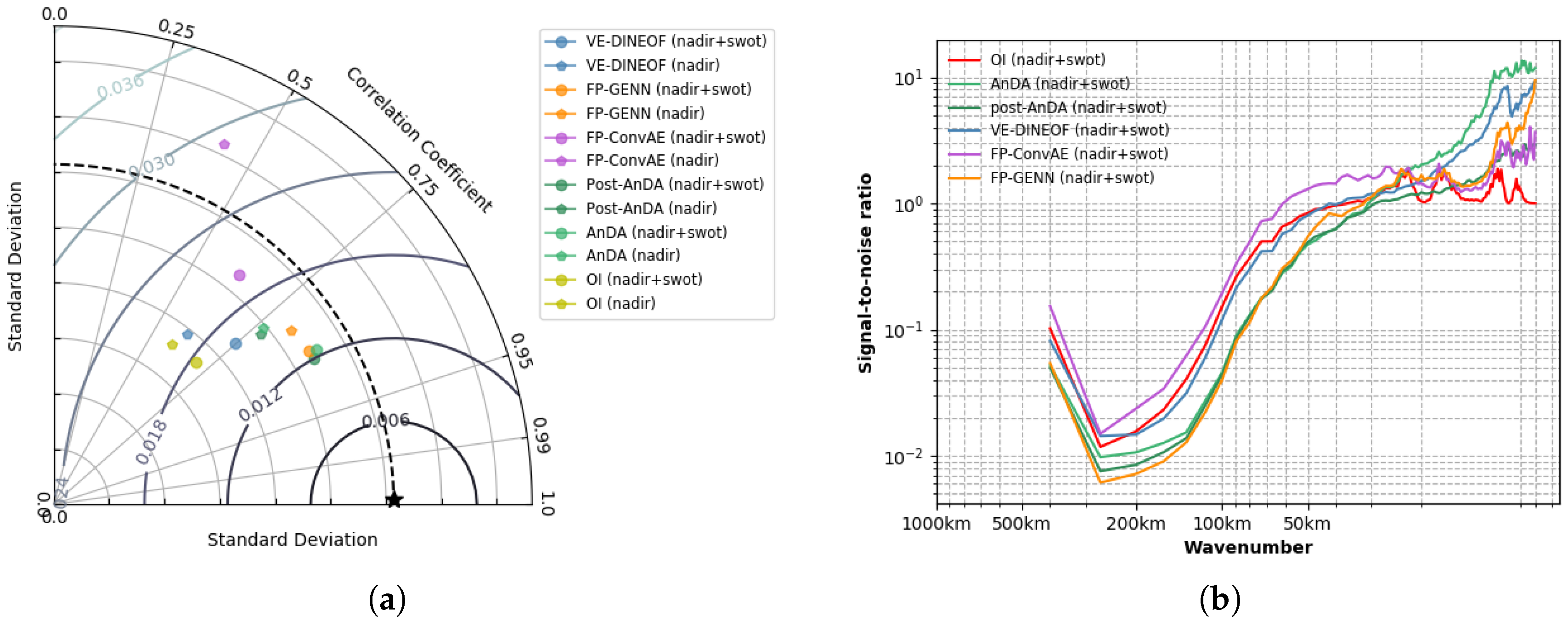
  • A significant contribution from the 2D spatial information provided by the additional SWOT sampling to improve the reconstruction of altimetric fields with a relative gain up to 30% in the SSH daily mean squared error, when compared to the single use of along-track nadir 1D information. Within this combined use of the two datasets, the spectral analysis indicates the new capability to reconstruct spatial scales up to 50–60 km which is an important improvement compared to the scales that OI is handling by now; on the other hand, the temporal sampling being less important than nadir tracks, in particular on the GULFSTREAM domain where periods of several days without any SWOT information appears, the reconstruction on these specific periods is sometimes better when learning only with along-track nadir as inputs: we believe that a longer training period (not available here) should improve the behavior of the NN on this specific issue.
  • The possibility for neural network methods to learn from the single observations, without requiring any numerical simulations, which is of particular interest on low latitude areas where the Rossby radius of deformation is large, thereby requesting an important catalog to efficiently retrieve the SSH dynamics over the year.
As it stands, the results obtained are very encouraging: FP-GENN is a “plug-and-play” algorithm whose conceptual use easily enables its implementation on new datasets. Many perspectives have to be considered in the short and medium terms.
The configuration of FP-GENN used here aims at minimizing the difference between the true anomaly state of the system d x and its representation ψ ( d x ) through energy form | | d x ψ ( d x ) | | 2 . Alternate energy forms have to be investigated, considering extremes or more generally the whole pdf. In addition, the fixed-point solver used in the joint interpolation approach with GENN never goes too far from the observations, even though they are noisy, which can be an issue in cases of strong noise, including spatial and/or temporal correlations, which was already seen when using SWOT data without any preprocessing (not shown here).
From a methodological point of view, the next developments are expected in the coming related works to increase the gain already observed with FP-GENN:
  • Use a joint learning of the dynamical representation ψ and the solver Γ , minimizing its reconstruction error. A significant gain in the reconstruction performance is expected according to preliminary results obtained with toy models [16].
  • A stochastic extension of GENN for including in the NN-based framework an estimation of the uncertainties, thereby enabling this new reconstruction method to fully compete with the other interpolators in a “data assimilation” context, with a possible link whith Gaussian processes and the related stochastic PDE formalism [18,19].
Besides methodological aspects, new applications are also promising. If we focus here on small North Atlantic subdomains, the transfer of the NN-based interpolators to an operational process chain would mean reproducing a similar work on the whole basin wherein the computational constraints in this learning-based setting with a large number of parameters would still be a challenge. Using a deep learning multi-GPU framework and building a pre-operational demonstrator should be of great interest in the community, as are other SWOT use cases, e.g., using pre-learning on SWOT data to produce a new interpolation of historical along-track nadir datasets, or taking advantage of the SWOT fast-sampling phase data as inputs for learning prior to its use with SWOT upcoming “operational” data. Last, because the 2D information brought by SWOT showed a significant gain in the reconstruction, a natural extension of this work would be to consider pseudo-observations SKIM datasets [20], whose swath width is more than twice larger (110 vs. 270 km), and another would be to propose multivariate analyses, including complementary datasets (SST/SSS), already existing in other data-driven schemes such as AnDA, with an easy extension as additional channels in a neural networks framework.

Supplementary Materials

The code is available on https://github.com/CIA-Oceanix/DINAE_keras with additional information provided in the ReadMe file to describe the architecture of the code and how to use it.

Author Contributions

Conceptualization, R.F. and M.B. (Maxime Beauchamp); methodology, R.F. and M.B. (Maxime Beauchamp); software, R.F. and M.B. (Maxime Beauchamp); validation, M.B. (Maxime Beauchamp); investigation, M.B. (Maxime Beauchamp), R.F., C.U., M.B. (Maxime Ballarotta) and B.C.; writing—original draft preparation, M.B. (Maxime Beauchamp). All authors have read and agreed to the published version of the manuscript.

Funding

Funding for the authors was provided by CNES (French Space Agency) through OSTST project MANATEE and SWOT ST project DIEGO. This work was also supported by ANR through project Melody and AI Chair OceaniX. It also benefited from HPC and GPU resources from Azure (Microsoft EU Ocean awards) and from GENCI-IDRIS (Grant No. 2020-101030). Special thanks to the French ANR project BOOST-SWOT for providing the datasets used in this work.

Conflicts of Interest

The authors declare no conflict of interest.

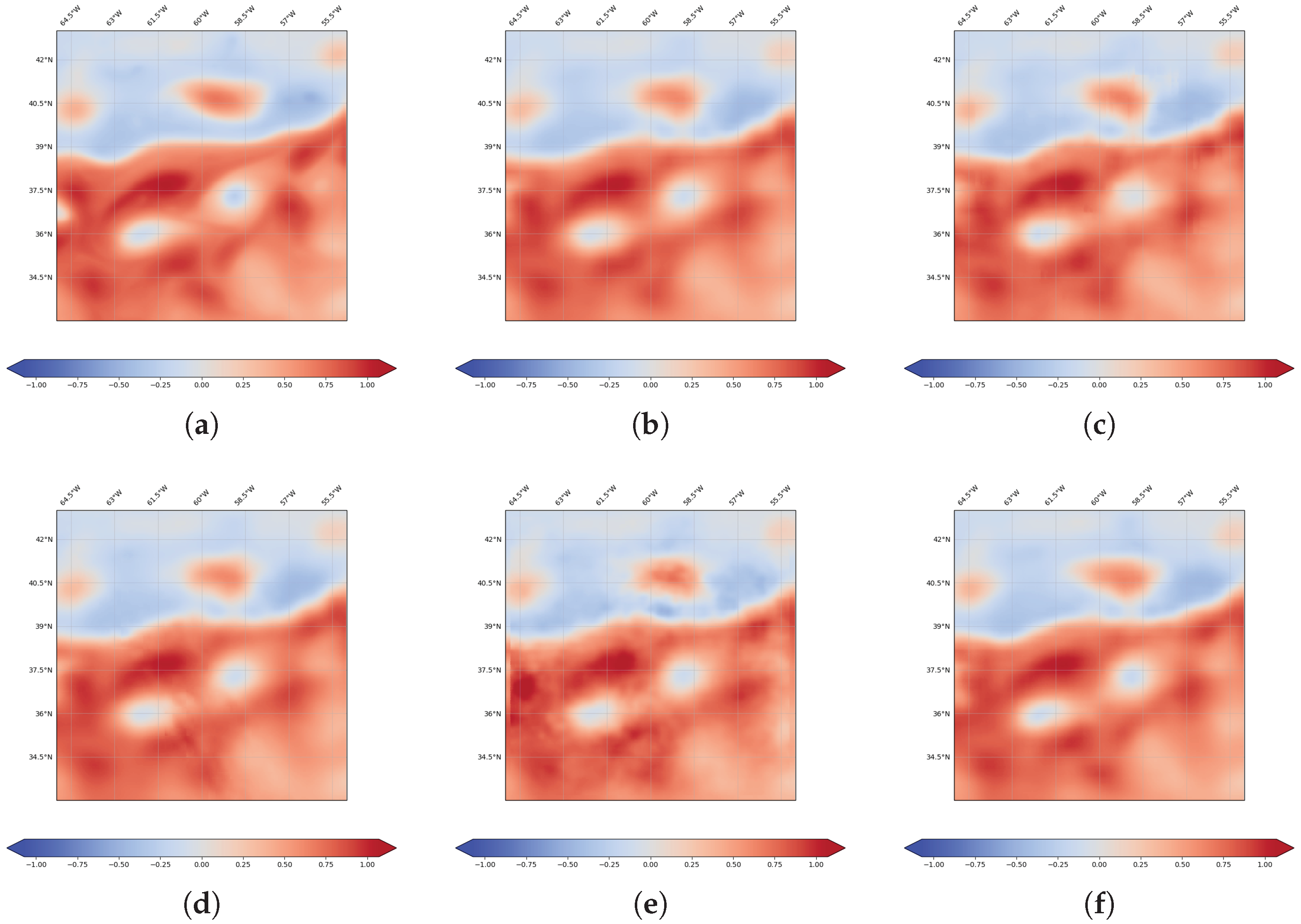
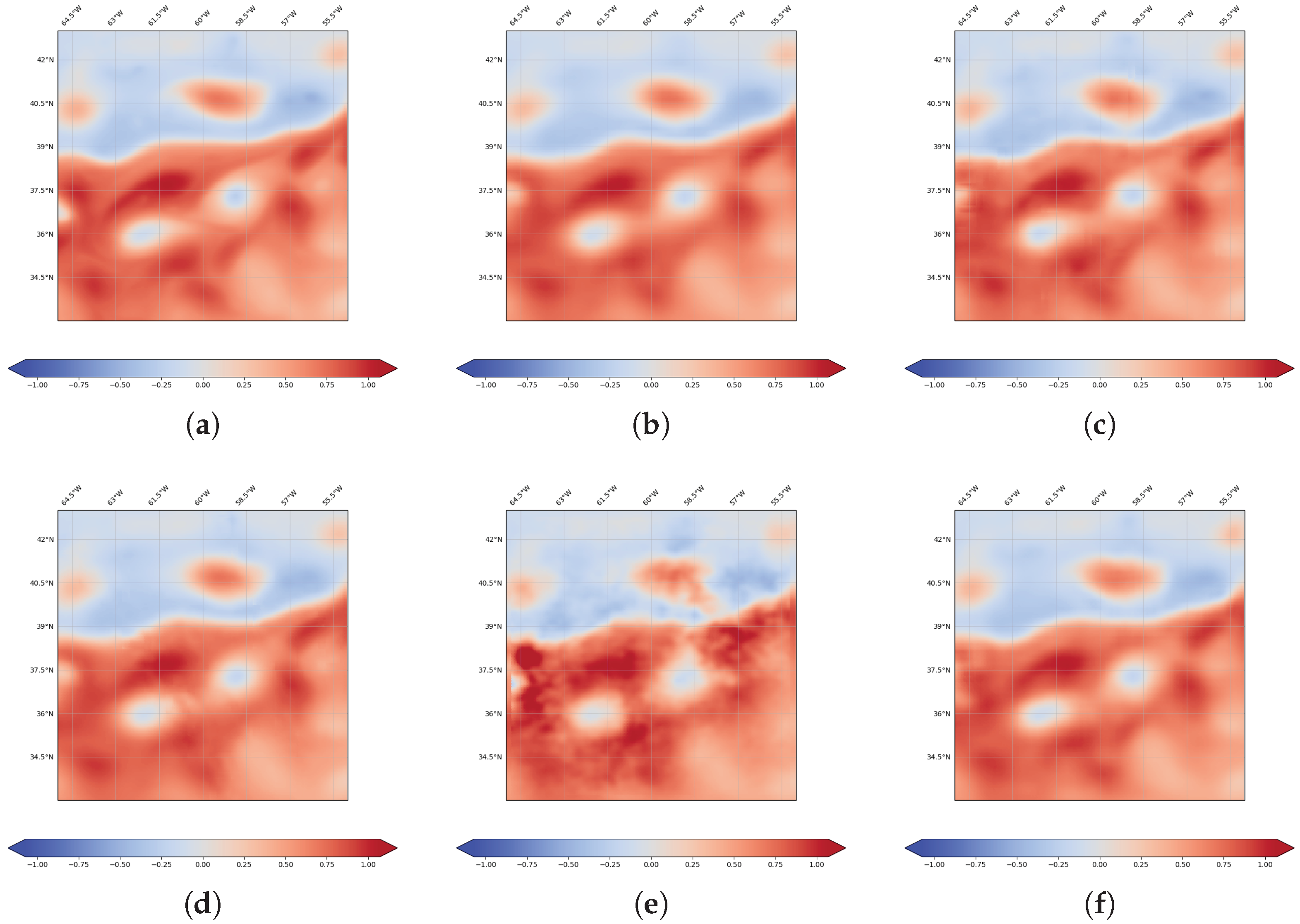
Appendix A. Complementary Figures for SSH Interpolations

Appendix A.1. GULFSTREAM

Figure A1. Global SSH field reconstruction (meters) obtained by OI, (post-)AnDA, VE-DINEOF, FP-ConvAE and FP-GENN using along-track nadir data only. (a) Ground truth (SSH), (b) OI, (c) post-AnDA, (d) VE-DINEOF, (e) FP-ConvAE, (f) FP-GENN.
Remotesensing 12 03806 g0a1
Figure A2. Global SSH field reconstruction (meters) obtained by OI, (post-)AnDA, VE-DINEOF, FP-ConvAE and FP-GENN for a joint assimilation/learning of along-track nadir with wide-swath SWOT data. (a) Ground truth (SSH), (b) OI, (c) post-AnDA, (d) VE-DINEOF, (e) FP-ConvAE, (f) FP-GENN.
Remotesensing 12 03806 g0a2

Appendix A.2. OSMOSIS

Figure A3. Global SSH field reconstruction (meters) obtained by OI, (post-)AnDA, VE-DINEOF, FP-ConvAE and FP-GENN using along-track nadir data only. (a) Ground truth (SSH), (b) OI, (c) post-AnDA, (d) VE-DINEOF, (e) FP-ConvAE, (f) FP-GENN.
Remotesensing 12 03806 g0a3
Figure A4. Global SSH field reconstruction (meters) obtained by OI, (post-)AnDA, VE-DINEOF, FP-ConvAE and FP-GENN for a joint assimilation/learning of along-track nadir with wide-swath SWOT data. (a) Ground truth (SSH), (b) OI, (c) post-AnDA, (d) VE-DINEOF, (e) FP-ConvAE, (f) FP-GENN.
Remotesensing 12 03806 g0a4

Appendix B. OSSE without Observation Errors

Appendix B.1. GULFSTREAM

Figure A5. Daily spatial nRMSE computed for the four 20-day non-continuous validation periods for the six supervised/unsupervised FP-GENN configurations. The spatial coverage of 11 days ( d = 5 ) accumulated along-track nadir (a) expanded with wide-swath SWOT data (b) is provided by the red barplot. (a) Nadir, (b) nadir+swot.
Remotesensing 12 03806 g0a5
Figure A6. Daily spatial nRMSE computed for the four 20-day non-continuous validation periods for OI, (post-)AnDA, VE-DINEOF, FP-ConvAE and FP-GENN. The spatial coverage of one day ( d = 0 ) accumulated along-track nadir and that of wide-swath SWOT data are respectively provided by the red and green barplots. (a) Nadir, (b) nadir+swot.
Remotesensing 12 03806 g0a6
Figure A7. Taylor diagram and signal-to-noise ratio computed for the four 20-day non-continuous validation periods for OI, (post-)AnDA, VE-DINEOF, FP-ConvAE and FP-GENN computed for both nadir use only and joint assimilation/learning with wide-swath SWOT data. (a) Taylor diagram, (b) Signal-to-noise ratio.
Remotesensing 12 03806 g0a7
Table A1. SSH and SSH gradient field R/I/AE-scores computed for the four 20-day non-continuous validation periods for OI, (post-)AnDA, VE-DINEOF, FP-ConvAE and FP-GENN for both nadir use only and joint assimilation/learning with wide-swath SWOT data.
Model TypeR-ScoreI-ScoreAE-Score Model TypeR-ScoreI-ScoreAE-Score
nadirOI86.5372.25_nadir OI 76.1472.41_
AnDA90.5676.81_ AnDA 81.8176.15_
VE-DINEOF91.3372.58_ VE DINEOF 80.0972.07_
FP-ConvAE69.4663.8279.86 FP ConvAE 58.3059.7970.14
FP-GENN95.1591.2896.32 FP GENN 84.7584.6388.05
nadir + SWOTOI91.7675.30_nadir + SWOT OI 71.4172.31_
AnDA91.7282.43_ AnDA 85.8579.80_
VE-DINEOF92.4776.00_ VE DINEOF 84.7373.36_
FP-ConvAE42.7834.9679.93 FP ConvAE 31.7836.4869.72
FP-GENN97.3191.4596.87 FP GENN 87.7585.3589.50
Figure A8. Global SSH field reconstruction (meters) obtained by OI, (post-)AnDA, VE-DINEOF, FP-ConvAE and FP-GENN using along-track nadir data only. (a) Ground truth (SSH), (b) OI, (c) post-AnDA, (d) VE-DINEOF, (e) FP-ConvAE, (f) FP-GENN.
Remotesensing 12 03806 g0a8
Figure A9. Global SSH gradient field reconstruction obtained by OI, (post-)AnDA, VE-DINEOF, FP-ConvAE and FP-GENN using along-track nadir data only. (a) Ground truth ( SSH ), (b) OI, (c) post-AnDA, (d) VE-DINEOF, (e) FP-ConvAE, (f) FP-GENN.
Remotesensing 12 03806 g0a9
Figure A10. Global SSH field reconstruction (meters) obtained by OI, (post-)AnDA, VE-DINEOF, FP-ConvAE and FP-GENN for a joint assimilation/learning of along-track nadir with wide-swath SWOT data. (a) Ground truth (SSH), (b) OI, (c) post-AnDA, (d) VE-DINEOF, (e) FP-ConvAE, (f) FP-GENN.
Remotesensing 12 03806 g0a10
Figure A11. Global SSH gradient field reconstruction obtained by OI, (post-)AnDA, VE-DINEOF, FP-ConvAE and FP-GENN for a joint assimilation/learning of along-track nadir with wide-swath SWOT data. (a) Ground truth ( SSH ), (b) OI, (c) post-AnDA, (d) VE-DINEOF, (e) FP-ConvAE, (f) FP-GENN.
Remotesensing 12 03806 g0a11

Appendix B.2. OSMOSIS

Figure A12. Daily spatial nRMSE computed for the four 20-day non-continuous validation periods for the six supervised/unsupervised FP-GENN configurations. The spatial coverage of 11 days ( d = 5 ) accumulated along-track nadir (a) expanded with wide-swath SWOT data (b) is provided by the red barplot. (a) Nadir, (b) nadir+swot.
Remotesensing 12 03806 g0a12
Figure A13. Daily spatial nRMSE computed for the four 20-day non-continuous validation periods for OI, (post-)AnDA, VE-DINEOF, FP-ConvAE and FP-GENN. The spatial coverage of one day ( d = 0 ) accumulated along-track nadir and that of wide-swath SWOT data are respectively provided by the red and green barplots. (a) Nadir, (b) nadir+swot.
Remotesensing 12 03806 g0a13
Table A2. SSH and SSH gradient field R/I/AE-scores computed for the four 20-day non-continuous validation periods for OI, (post-)AnDA, VE-DINEOF, FP-ConvAE and FP-GENN for both nadir use only and joint assimilation/learning with wide-swath SWOT data.
Model TypeR-ScoreI-ScoreAE-Score Model TypeR-ScoreI-ScoreAE-Score
nadirOI44.6334.93_nadir OI 49.5348.20_
AnDA76.6059.42_ AnDA 64.5659.88_
VE-DINEOF77.1737.66_ VE DINEOF 58.7145.61_
FP-ConvAE28.3917.0042.94 FP ConvAE 22.4719.1236.66
FP-GENN84.3576.1786.30 FP GENN 62.4761.6464.88
nadir + SWOTOI54.3147.87_nadir + SWOT OI 37.5547.93_
AnDA83.0774.95_ AnDA 75.1370.22_
VE-DINEOF83.4751.50_ VE DINEOF 79.3149.32_
FP-ConvAE36.8033.3747.56 FP ConvAE 30.8535.0639.06
FP-GENN90.6781.3588.04 FP GENN 67.9967.4769.21
Figure A14. Taylor diagram and signal-to-noise ratio computed for the four 20-day non-continuous validation periods for OI, (post-)AnDA, VE-DINEOF, FP-ConvAE and FP-GENN computed for both nadir use only and joint assimilation/learning with wide-swath SWOT data. (a) Taylor diagram, (b) Signal-to-noise ratio.
Remotesensing 12 03806 g0a14
Figure A15. Global SSH field reconstruction (meters) obtained by OI, (post-)AnDA, VE-DINEOF, FP-ConvAE and FP-GENN using along-track nadir data only. (a) Ground truth (SSH), (b) OI, (c) post-AnDA, (d) VE-DINEOF, (e) FP-ConvAE, (f) FP-GENN.
Remotesensing 12 03806 g0a15
Figure A16. Global SSH gradient field reconstruction obtained by OI, (post-)AnDA, VE-DINEOF, FP-ConvAE and FP-GENN using along-track nadir data only. (a) Ground truth ( SSH ), (b) OI, (c) post-AnDA, (d) VE-DINEOF, (e) FP-ConvAE, (f) FP-GENN.
Remotesensing 12 03806 g0a16
Figure A17. Global SSH field reconstruction (meters) obtained by OI, (post-)AnDA, VE-DINEOF, FP-ConvAE and FP-GENN for a joint assimilation/learning of along-track nadir with wide-swath SWOT data. (a) Ground truth (SSH), (b) OI, (c) post-AnDA, (d) VE-DINEOF, (e) FP-ConvAE, (f) FP-GENN.
Remotesensing 12 03806 g0a17
Figure A18. Global SSH gradient field reconstruction obtained by OI, (post-)AnDA, VE-DINEOF, FP-ConvAE and FP-GENN for a joint assimilation/learning of along-track nadir with wide-swath SWOT data. (a) Ground truth ( SSH ), (b) OI, (c) post-AnDA, (d) VE-DINEOF, (e) FP-ConvAE, (f) FP-GENN.
Remotesensing 12 03806 g0a18

References

  1. Ballarotta, M.; Ubelmann, C.; Pujol, M.I.; Taburet, G.; Fournier, F.; Legeais, J.F.; Faugère, Y.; Delepoulle, A.; Chelton, D.; Dibarboure, G.; et al. On the resolutions of ocean altimetry maps. Ocean Sci. 2019, 15, 1091–1109. [Google Scholar] [CrossRef] [Green Version]
  2. Lguensat, R.; Tandeo, P.; Aillot, P.; Fablet, R. The Analog Data Assimilation. Mon. Weather Rev. 2017, 145, 4093–4107. [Google Scholar] [CrossRef] [Green Version]
  3. Lguensat, R.; Huynh Viet, P.; Sun, M.; Chen, G.; Fenglin, T.; Chapron, B.; Fablet, R. Data-driven Interpolation of Sea Level Anomalies using Analog Data Assimilation. Remote Sens. 2017, 11, 858. [Google Scholar] [CrossRef] [Green Version]
  4. Fablet, R.; Viet, P.H.; Lguensat, R. Data-Driven Models for the Spatio-Temporal Interpolation of Satellite-Derived SST Fields. IEEE Trans. Comput. Imaging 2017, 3, 647–657. [Google Scholar] [CrossRef]
  5. Lopez-Radcenco, M.; Pascual, A.; Gomez-Navarro, L.; Aissa-El-Bey, A.; Chapron, B.; Fablet, R. Analog Data Assimilation of Along-Track Nadir and Wide-Swath SWOT Altimetry Observations in the Western Mediterranean Sea. IEEE J. Sel. Top. Appl. Earth Obs. Remote Sens. 2019, 1–11. [Google Scholar] [CrossRef]
  6. Ouala, S.; Fablet, R.; Herzet, C.; Chapron, B.; Pascual, A.; Collard, F.; Gaultier, L. Neural Network Based Kalman Filters for the Spatio-Temporal Interpolation of Satellite-Derived Sea Surface Temperature. Remote Sens. 2018, 10, 1864. [Google Scholar] [CrossRef] [Green Version]
  7. Taburet, G.; Sanchez-Roman, A.; Ballarotta, M.; Pujol, M.I.; Legeais, J.F.; Fournier, F.; Faugere, Y.; Dibarboure, G. DUACS DT2018: 25 years of reprocessed sea level altimetry products. Ocean Sci. 2019, 15, 1207–1224. [Google Scholar] [CrossRef] [Green Version]
  8. Molines, J.M. Meom-Configurations/NATL60-CJM165: NATL60 Code Used for CJM165 Experiment; Zenodo: Geneva, Switzerland, 2018. [Google Scholar] [CrossRef]
  9. Dufau, C.; Orsztynowicz, M.; Dibarboure, G.; Morrow, R.; Le Traon, P.Y. Mesoscale resolution capability of altimetry: Present and future. J. Geophys. Res. Ocean. 2016, 121, 4910–4927. [Google Scholar] [CrossRef] [Green Version]
  10. Gaultier, L.; Ubelmann, C.; Fu, L.L. The Challenge of Using Future SWOT Data for Oceanic Field Reconstruction. J. Atmos. Ocean. Technol. 2015, 33, 119–126. [Google Scholar] [CrossRef]
  11. Esteban-Fernandez, D. SWOT Project Mission Performance and Error Budget Document; Technical Report; JPL, NASA: Pasadena, CA, USA, 2014. [Google Scholar]
  12. Gaultier, L.; Ubelmann, C. SWOT Simulator Documentation; Technical Report; JPL, NASA: Pasadena, CA, USA, 2010. [Google Scholar]
  13. Metref, S.; Cosme, E.; Le Guillou, F.; Le Sommer, J.; Brankart, J.M.; Verron, J. Wide-Swath Altimetric Satellite Data Assimilation With Correlated-Error Reduction. Front. Mar. Sci. 2020, 6, 822. [Google Scholar] [CrossRef] [Green Version]
  14. Ping, B.; Su, F.; Meng, Y. An Improved DINEOF Algorithm for Filling Missing Values in Spatio-Temporal Sea Surface Temperature Data. PLoS ONE 2016, 11, e0155928. [Google Scholar] [CrossRef] [PubMed] [Green Version]
  15. Fablet, R.; Drumetz, L.; Rousseau, F.; Beauchamp, M. Joint Interpolation and Representation Learning for Irregularly-Sampled Satellite-Derived Geophysical Fields; IMT Atlantique: Brest, France, 2020. [Google Scholar]
  16. Fablet, R.; Drumetz, L.; Rousseau, F. Joint learning of variational representations and solvers for inverse problems with partially-observed data. arXiv 2020, arXiv:2006.03653. [Google Scholar]
  17. Welch, P. The use of fast Fourier transform for the estimation of power spectra: A method based on time averaging over short, modified periodograms. IEEE Trans. Audio Electroacoust. 1967, 15, 70–73. [Google Scholar] [CrossRef] [Green Version]
  18. Lindgren, F.; Rue, H.; Lindström, J. An explicit link between Gaussian fields and Gaussian Markov random fields: The stochastic partial differential equation approach. J. R. Stat. Soc. Ser. B (Stat. Methodol.) 2011, 73, 423–498. [Google Scholar] [CrossRef] [Green Version]
  19. Sidén, P.; Lindsten, F. Deep Gaussian Markov random fields. arXiv 2020, arXiv:2002.07467. [Google Scholar]
  20. Ardhuin, F.; Brandt, P.; Gaultier, L.; Donlon, C.; Battaglia, A.; Boy, F.; Casal, T.; Chapron, B.; Collard, F.; Cravatte, S.; et al. SKIM, a Candidate Satellite Mission Exploring Global Ocean Currents and Waves. Front. Mar. Sci. 2019. [Google Scholar] [CrossRef] [Green Version]
Figure 1. GULFSTREAM and OSMOSIS domains.
Remotesensing 12 03806 g001
Figure 2. One ( d = 0 ) and 11 day ( d = 5 ) accumulated along-track nadir and wide-swath SSH pseudo-observations (meters) on 4 August 2013 (a,b) and 5 August 2013 (c,d). (a) Nadir (d = 0), (b) nadir (d = 0) + swot, (c) nadir (d = 5), (d) nadir (d = 5) + swot.
Remotesensing 12 03806 g002
Figure 3. Variance of the observation error ε k as a function of the hourly lag between the observations y k and the day to estimation time t k . Blue barplots are the conditional distributions of ε k according to hourly time lag; dotted red lines are their variances and a solid black line is the corresponding parametric fit.
Remotesensing 12 03806 g003
Figure 4. Sketch of the iterative fixed-point algorithm.
Remotesensing 12 03806 g004
Figure 5. Daily spatial nRMSE computed over the four 20-day non-continuous validation periodss for the six supervised/unsupervised FP-GENN configurations. The spatial coverage of 11 days ( d = 5 ) accumulated along-track nadir (a) expanded with wide-swath SWOT data (b) is provided by the red barplot. (a) Nadir, (b) nadir+swot.
Remotesensing 12 03806 g005
Figure 6. Daily spatial nRMSE computed for the four 20-day non-continuous validation periodss for OI, (post-)AnDA, VE-DINEOF, FP-ConvAE and FP-GENN. The spatial coverage of one day ( d = 0 ) accumulated along-track nadir and that of wide-swath SWOT data are respectively provided by the red and green barplots. (a) Nadir, (b) nadir+swot.
Remotesensing 12 03806 g006
Figure 7. Taylor diagram and signal-to-noise ratio computed for the four 20-day non-continuous validation periods for OI, (post-)AnDA, VE-DINEOF, FP-ConvAE and FP-GENN computed for both nadir use only and joint assimilation/learning with wide-swath SWOT data. (a) Taylor diagram, (b) signal-to-noise ratio.
Remotesensing 12 03806 g007
Figure 8. Global SSH gradient field reconstruction obtained by OI, (post-)AnDA, VE-DINEOF, FP-ConvAE and FP-GENN using along-track nadir data only. (a) Ground truth ( SSH ), (b) OI, (c) post-AnDA, (d) VE-DINEOF, (e) FP-ConvAE, (f) FP-GENN.
Remotesensing 12 03806 g008
Figure 9. Global SSH gradient field reconstruction obtained by OI, (post-)AnDA, VE-DINEOF, FP-ConvAE and FP-GENN for a joint assimilation/learning of along-track nadir with wide-swath SWOT data. (a) Ground truth ( SSH ), (b) OI, (c) post-AnDA, (d) VE-DINEOF, (e) FP-ConvAE, (f) FP-GENN.
Remotesensing 12 03806 g009
Figure 10. One ( d = 0 ) and 11 day ( d = 5 ) accumulated along-track nadir and wide-swath SSH pseudo-observations (meters) on 4 August 2013 (a,b) and 5 August 2013 (c,d). (a) Nadir (d = 0), (b) nadir (d = 0) + swot, (c) nadir (d = 5), (d) nadir (d = 5) + swot.
Remotesensing 12 03806 g010
Figure 11. Daily spatial nRMSE computed for the four 20-day non-continuous validation periods for the six supervised/unsupervised FP-GENN configurations. The spatial coverage of 11 days ( d = 5 ) accumulated along-track nadir (a) expanded with wide-swath SWOT data, (b) is provided by the red barplot. (a) Nadir, (b) nadir+swot.
Remotesensing 12 03806 g011
Figure 12. Daily spatial nRMSE computed for the four 20-day non-continuous validation periods for OI, (post-)AnDA, VE-DINEOF, FP-ConvAE and FP-GENN. The spatial coverage of one day ( d = 0 ) accumulated along-track nadir and that of wide-swath SWOT data are respectively provided by the red and green barplots. (a) Nadir, (b) nadir+swot.
Remotesensing 12 03806 g012
Figure 13. Taylor diagram and signal-to-noise ratio computed for the four 20-day non-continuous validation periods for OI, (post-)AnDA, VE-DINEOF, FP-ConvAE and FP-GENN computed for both nadir use only and joint assimilation/learning with wide-swath SWOT data. (a) Taylor diagram, (b) signal-to-noise ratio.
Remotesensing 12 03806 g013
Figure 14. Global SSH gradient field reconstruction obtained by OI, (post-)AnDA, VE-DINEOF, FP-ConvAE and FP-GENN using along-track nadir data only. (a) Ground truth ( SSH ), (b) OI, (c) post-AnDA, (d) VE-DINEOF, (e) FP-ConvAE, (f) FP-GENN.
Remotesensing 12 03806 g014
Figure 15. Global SSH gradient field reconstruction obtained by OI, (post-)AnDA, VE-DINEOF, FP-ConvAE and FP-GENN for a joint assimilation/learning of along-track nadir with wide-swath SWOT data. (a) Ground truth ( SSH ), (b) OI, (c) post-AnDA, (d) VE-DINEOF, (e) FP-ConvAE, (f) FP-GENN.
Remotesensing 12 03806 g015
Table 1. Temporal and spectral statistics used to assess the performances of the interpolators in the observation system simulation experiment.
NameFormula
nRMSEnRMSE( t k ) = 1 | D ˜ | D ˜ ( x k x ^ k ) 2 / σ x
Error variance σ x x ^ 2 ( t k ) = 1 | D ˜ | D ˜ ( x k x ^ k ) ( x k x ^ k ) ¯ 2
CorrelationCOR( t k ) = Cov ( x k , x ^ k ) σ ( x k ) σ ( x ^ k )
Temporal domainReconstruction scoreR-score = 100 × 1 Ω ( ( x x ¯ ) ( x ^ x ^ ¯ ) ) 2 Ω ( x x ¯ ) 2
Interpolation scoreI-score = 100 × 1 Ω ¯ ( ( x x ¯ ) ( x ^ x ^ ¯ ) ) 2 Ω ¯ ( x x ¯ ) 2
Auto-encoder scoreAE-score = 100 × 1 D ˜ ( ( x x ¯ ) ( ψ ( x ) ψ ( x ) ¯ ) ) 2 D ˜ ( x x ¯ ) 2
Spectral domainRAPSRAPS( λ ) = DSP ( x ^ k ) ( λ )
Signal-to-Noise RatioSNR( λ ) = DSP ( x k x ^ k ) ( λ ) DSP ( x k ) ( λ )
Table 2. Specifications of GENN learning-based strategies.
ConfigurationsData
ObservationsGap-Free MapsDUACS OI
Supervised 1Input 🗸yes/no
Target 🗸
Supervised 2Input🗸 yes/no
Target 🗸
UnsupervisedInput🗸 yes/no
Target🗸
Table 3. Sea surface height (SSH) and SSH gradient field R/I/AE-scores computed for the four 20-day non-continuous validation periods for OI, (post-)AnDA, VE-DINEOF, FP-ConvAE and FP-GENN for both nadir use only and joint assimilation/learning with wide-swath SWOT data.
Model TypeR-ScoreI-ScoreAE-Score Model TypeR-ScoreI-ScoreAE-Score
nadirOI87.3272.17_nadir OI 78.0375.97_
AnDA94.8577.91_ AnDA 85.5679.14_
VE-DINEOF96.1172.72_ VE DINEOF 82.6975.61_
FP-ConvAE87.8276.3282.85 FP ConvAE 77.8076.8175.89
FP-GENN91.7884.5693.15 FP GENN 81.0580.5684.24
nadir + SWOTOI93.2574.25_nadir + SWOT OI 73.8375.78
AnDA96.0583.55_ AnDA 89.8982.88_
VE-DINEOF97.1375.28_ VE DINEOF 88.1976.69_
FP-ConvAE80.6377.5183.26 FP ConvAE 76.2076.4975.84
FP-GENN96.4990.1395.58 FP GENN 86.9685.3388.23
Table 4. SSH and SSH gradient field R/I/AE-scores computed for the four 20-day non-continuous validation periods for OI, (post-)AnDA, VE-DINEOF, FP-ConvAE and FP-GENN for both nadir use only and joint assimilation/learning with wide-swath SWOT data.
Model TypeR-ScoreI-ScoreAE-Score Model TypeR-ScoreI-ScoreAE-Score
nadirOI42.0532.11_nadir OI 48.8347.57_
AnDA58.8547.02_ AnDA 58.7855.17_
VE-DINEOF26.2930.61_ VE DINEOF 33.1135.28_
FP-ConvAE37.2031.6747.77 FP ConvAE 32.1535.8741.24
FP-GENN67.9462.5280.40 FP GENN 50.5352.1260.41
nadir + SWOTOI54.2147.75_nadir + SWOT OI 36.8347.30_
AnDA81.1570.91_ AnDA 72.3567.59_
VE-DINEOF69.0832.98_ VE DINEOF 22.0824.90_
FP-ConvAE45.1542.7047.93 FP ConvAE 38.2243.1342.03
FP-GENN77.1669.5683.08 FP GENN 56.2959.2167.69
Publisher’s Note: MDPI stays neutral with regard to jurisdictional claims in published maps and institutional affiliations.

