Rapid Assessment of Hillslope Erosion Risk after the 2019–2020 Wildfires and Storm Events in Sydney Drinking Water Catchment

Abstract

The Australian Black Summer wildfires between September 2019 and January 2020 burnt many parts of eastern Australia including major forests within the Sydney drinking water catchment (SDWC) area, almost 16.000 km². There was great concern on post-fire erosion and water quality hazards to Sydney’s drinking water supply, especially after the heavy rainfall events in February 2020. We developed a rapid and innovative approach to estimate post-fire hillslope erosion using weather radar, remote sensing, Google Earth Engine (GEE), Geographical Information Systems (GIS), and the Revised Universal Soil Loss Equation (RUSLE). The event-based rainfall erosivity was estimated from radar-derived rainfall accumulations for all storm events after the wildfires. Satellite data including Sentinel-2, Landsat-8, and Moderate Resolution Imaging Spectroradiometer (MODIS) were used to estimate the fractional vegetation covers and the RUSLE cover-management factor. The study reveals that the average post-fire erosion rate over SDWC in February 2020 was 4.9 Mg ha⁻¹ month⁻¹, about 30 times higher than the pre-fire erosion and 10 times higher than the average erosion rate at the same period because of the intense storm events and rainfall erosivity with a return period over 40 years. The high post-fire erosion risk areas (up to 23.8 Mg ha⁻¹ month⁻¹) were at sub-catchments near Warragamba Dam which forms Lake Burragorang and supplies drinking water to more than four million people in Sydney. These findings assist in the timely assessment of post-fire erosion and water quality risks and help develop cost-effective fire incident management and mitigation actions for such an area with both significant ecological and drinking water assets. The methodology developed from this study is potentially applicable elsewhere for similar studies as the input datasets (satellite and radar data) and computing platforms (GEE, GIS) are available and accessible worldwide.

1. Introduction

Because of its mostly hot, dry, and erratic climate, wildfires in Australia and many parts of the world are frequently occurring events during the hotter months. Between 2017 and 2019, severe drought developed across much of eastern and inland Australia including Queensland, New South Wales (NSW), and Victoria, also extending into parts of South Australia and Western Australia. As at late 2019, many regions of Australia were still in significant drought, contributing to water restrictions and extreme fire conditions [1]. The 2019–20 Australian bushfire season, colloquially known as the “Black Summer,” began with several serious uncontrolled fires in June 2019, an early start to the wildfire season as it normally starts in early October in NSW [2]. Throughout late 2019 and early 2020 these wildfires both multiplied and combined, to create mega fires that burnt predominantly throughout the southeast of the country, peaking during December–January, and having been since contained and/or extinguished [2,3,4].

In NSW, the three-year (2017–2019) severe drought had left forests tinder dry, facilitating rapid expansion of fires across the state. Sydney—the nation’s most populated city (about 5 million residents)—had been under water restrictions since late 2019, when its dams fell below 45% capacity. The wildfires in NSW between September 2019 to January 2020 (the 2019-20 fires) were unprecedented in their extent and intensity [4]. The NSW Rural Fire Service (RFS) reported that the 2019–2020 fires burnt 5.4 million hectares (including ~11,264 bush or grass fires across 6.7% of the State) and destroyed 2439 homes [3].

Wildfires not only create risk to lives, infrastructure, and properties, but also cause land and ecosystem degradation through increased soil erosion. The subsequent sediment deposition in rivers, lakes, and reservoirs is of great concern for drinking water quality, aquatic habitat, and environmental degradation. When large rainfall events occur in a short period of time, runoff will wash a lot of ash and sediment into waterways and dams. Rain also transports other contaminants, such as building debris, dead animals, and pollutants from fire retardant. Soil sediment, ash, and other contaminants pose a hazard to human health when mobilized in drinking water catchments. It is therefore necessary to quantitatively estimate soil erosion after severe wildfires in order to assess the extent and magnitude of post-fire soil erosion risk and the effectiveness of any rehabilitation or mitigation actions [5].

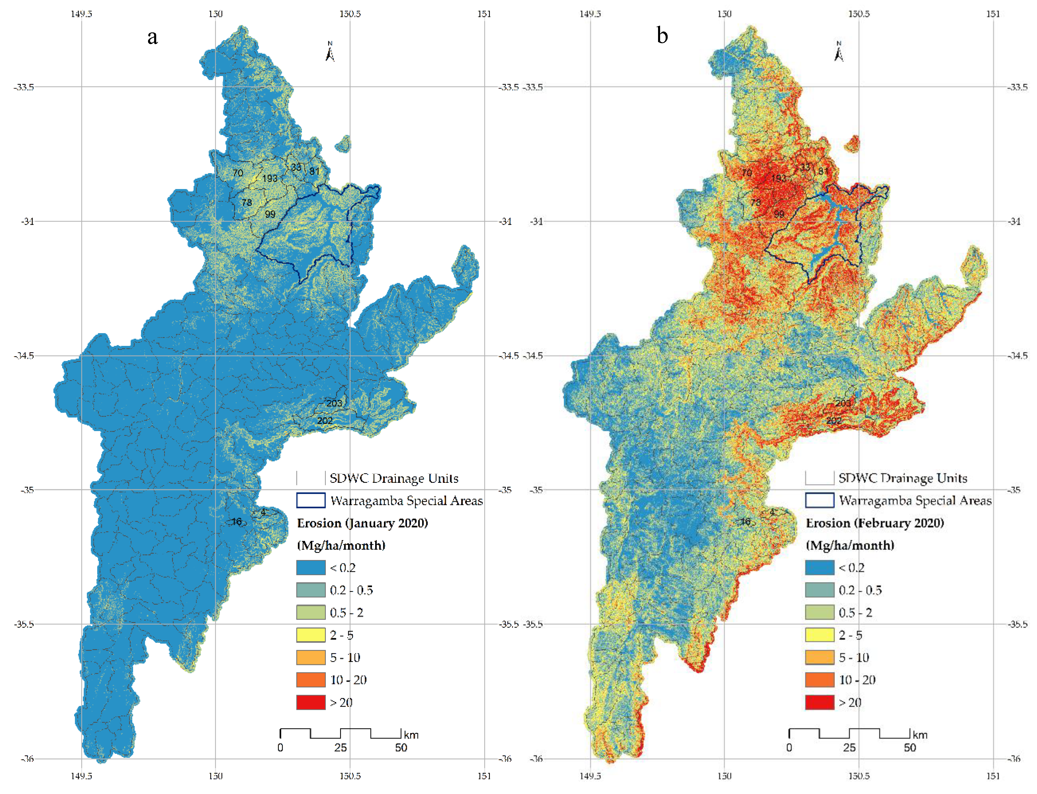
The Bureau of Meteorology (BoM) recorded 51 mm rainfall in January 2020 and 337 mm in February 2020 over the Sydney drinking water catchment (SDWC) areas. The rainfall events (especially in February) were widespread and helped extinguish the wildfires. However, the rainfall also caused severe runoff and hillslope erosion. As rainfall intensity is the leading agent contributing to greater erosion rates, and the subsequent effects on water quality, it is necessary to obtain timely rainfall information for fire recovery and erosion control practices. The rapid assessment of these risks and timely mitigation actions can significantly reduce risks to public safety, infrastructure, and the environment [5].

Hillslope erosion (including sheet and rill erosion) is the major form of water erosion and the dominant source of sediment in waterways in Australia and many parts of the world [5,6,7]. Monitoring of hillslope erosion after wildfires may be by direct measurement, such as flumes and sediment traps, or from tipping bucket sampling techniques. However, these techniques are commonly expensive, episodic, and impractical to apply across a large catchment. Observers with different levels of expertise make it difficult to consistently measure or predict long-term soil loss or erosion risk. A common model and consistent datasets are required for reliable soil loss prediction to provide consistent and continuous erosion information for short- and long-term soil and water quality management [5,6,7].

Many erosion models have been developed to predict soil loss in different regions in the world. Among them, the Universal Soil Loss Equation [8] or the revised USLE (RUSLE) [9] and Water Erosion Prediction Project (WEPP) [10] are widely used to estimate long-term average soil loss rates using rainfall, soil, topography, and land cover and management as inputs. These estimates have been used in long-term planning and soil condition assessment, and have been applied in Australia continent [11,12]. However, the impact of highly variable and extreme rainfall events cannot be estimated using the long-term averages erosion. Severe erosion and sediment transport are often caused by short but strong storm events [5,6].

It is increasingly important to construct an event-based erosion model to predict the extreme erosion risks given the predicted increase in climate variability and fire intensity [13]. Ideally, areas at risk of severe damage should be identified and prioritized for assessment and remediation in the event of fire [14,15], especially for drinking water catchments. Yet, there are few studies and applications of erosion models on estimation of storm event-based rainfall erosivity and erosion. One of the major limiting factors is the lack of rainfall data at high spatial and temporal resolutions, as well as computational capacity of large quantity of spatial data [16,17]. It remains a research challenge to provide quantitative and timely assessments of hillslope erosion after wildland fires during individual storm events to support water and catchment management [5].

Weather radar data have very high temporal resolution (15 min or less) and spatial resolution (1 km or less) with the potential for estimating event-based rainfall erosivity or the 30-min rainfall erosivity index (EI30). Such data sets have recently been applied in event-based erosion modeling to compute a spatial EI30 index [18] and to monitor erosion after wildfires at Warrumbungle National Park in NSW, Australia [5,6]. Its application over a large area or catchment at near real-time of rainfall events is still a research and implementation challenge. The emerging new technologies, such as machine learning, Google Earth Engine (GEE) processing, and high-resolution (spatial, spectral and temporal) satellite remote sensing, can be employed for the efficient implementation of the event-based erosion model, especially when large catchments or regions are concerned [19]. These together can provide timely erosion risk estimation that explicitly link soil loss and sedimentation with vegetation cover and land management, especially in events of wildfires and storms. The improved capability to predict impacts on water quality as a result of wildfires and erosion helps prioritize the mitigation actions in the drinking water catchments.

The aim of this study was to develop a rapid approach to assess the post-fire erosion in near real-time during storm events. We developed an integrated approach using the RUSLE, remote sensing, and Geographical Information System (GIS) to map the potential erosion risk over space and time, with the SDWC as the pilot study area. Water managers were able to use the results to prioritize monitoring points and areas for erosion assessment and interventions following storm events.

2. Materials and Methods

2.1. The Study Area

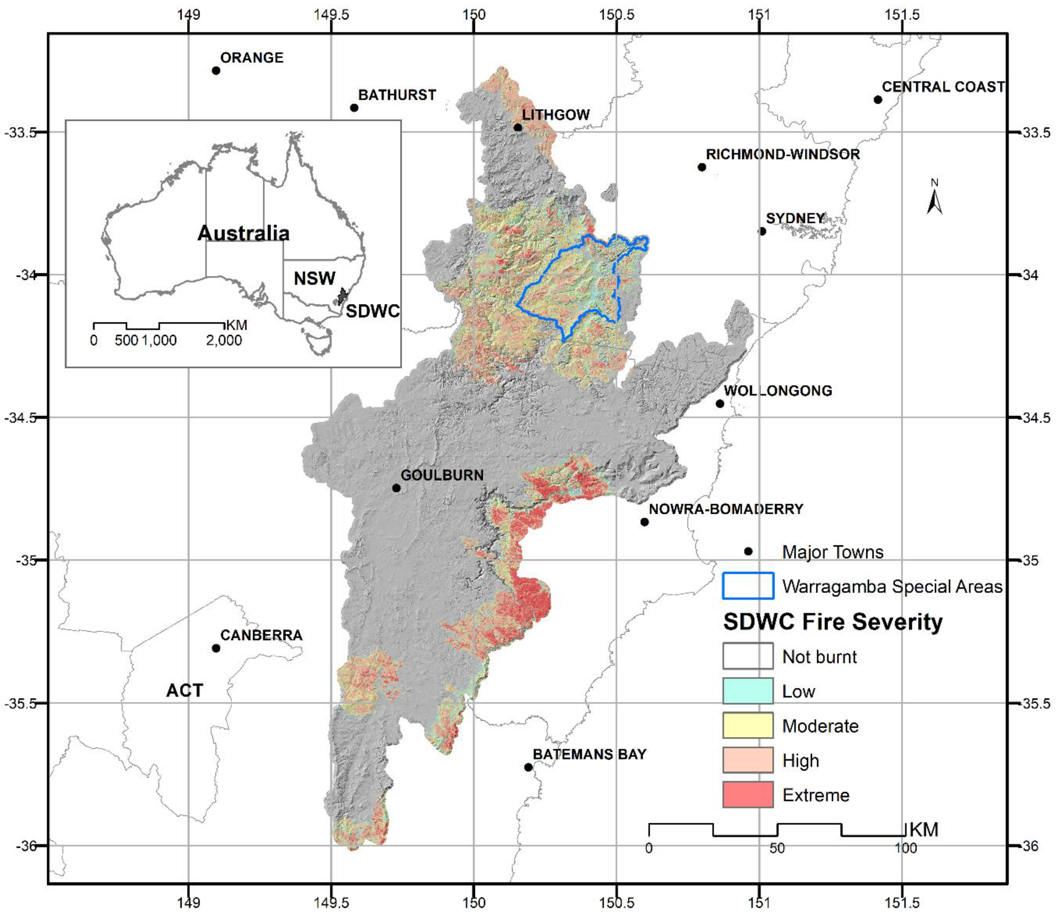
The SDWC area includes five main catchments and 204 sub-catchments (or drainage units). It extends from north of Lithgow in the upper Blue Mountains, to the source of the Shoalhaven River near Cooma in the south, and from Woronora in the east to the source of the Wollondilly River west of Crookwell. These catchments cover an area of almost 16,000 km², about seven times larger than the Australia Capital Territory (ACT) to its southwest (Figure 1). The dam across the Warragamba River forms Lake Burragorang which provides drinking water to Sydney and surrounding regions for more than five million people or 60 per cent of the NSW population.

The annual average rainfall in SDWC is about 841 mm based on the BoM gridded rainfall data [20] over the 30-year period between 1981 and 2010 (or “climate normals”) as used in climate maps and statistics in Australia and many parts of the world [21]. The rainfall in 2019 (before and during the 2019–2020 wildfire) is only about 473 mm which was far below the average. The SDWC area experiences significant seasonal variation in monthly rainfall. The months with the highest rainfalls are February (100 mm), November (85 mm), and January (79 mm). The months with least rainfalls are July (55 mm), September (57 mm), and August (59 mm) over the SDWC area.

The dominant land uses are livestock grazing (35%), nature conservation lands or national parks (30%), crown lands and reserves (16%), and others including intensive agriculture, horticulture, mining, and reservoirs (19%) based on the 2017 land use map over the SDWC area [22]. Soils types in SDWC are variable though strongly influenced by lithology and landform. Texture contrast soils with acidic subsoils (Kurosols) dominate the catchments (46%). Sandy soils with minimal soil development (Rudosols and Tenosol) are also common (30%) and often very shallow in steep-sloped terrain. The elevations range from 21 m to 1463 m (a.s.l) with an average slope of 16.7% over the SDWC area. The elevations range from 41 m to 1356 m (a.s.l) with an average slope of 28.7% at the sub-catchments near the Warragamba Dam and 70% of areas being mountainous terrain.

The 2019–2020 fires have severely and extensively burnt major forests within the drinking water catchments for Sydney, about 30% of SDWC areas have been burnt, and 16% of them are in high or extreme severity based on the fire extent and severity mapping (FESM) [23]. The fires were more severe near the Warragamba Dam, where about 81% of designated Special Areas burned (areas with little to no public access), with 30% at high to extreme fire severities (Figure 1). These drinking water catchments are managed by Water New South Wales (WaterNSW) and the New South Wales Department of Planning, Industry and Environment (DPIE).

2.2. The Datasets

The primary datasets used in this study were radar rainfall data, satellite images (Landsat-8 and Sentinel-2 with cloud cover < 5%), MODIS-derived fractional vegetation cover (FVC), fire severity, soil and water quality data. The Lansat-8 (OLI Level-2 surface reflectance) and Sentinel-2 (Level-2A BOA reflectance images) datasets for the 2019–2020 wildfire period were obtained via the Earth Engine Data Catalog [24]. The FVC datasets, derived from MODIS Nadir BRDF-Adjusted Reflectance product (MCD43A4) Collection 6, include monthly Photosynthetic Vegetation (PV), Non-Photosynthetic Vegetation (NPV), and Bare Soil (BS) at a spatial resolution of 500 m [25,26] were obtained online [27].

Obtaining clear satellite images at high resolution data, for SDWC area is difficult because of clouds and smokes during the 2019–2020 wildfire period. This problem was partially overcome by using Sentinel-2 with a more frequent (5-day) revisiting frequency. The Sentinel-2 multi-spectral instrument (MSI) sensor provides 13 spectral bands with a spatial resolution of 10–20 m in vegetation mapping. In addition, Sentinel-2 offers three new red edge spectral bands, which has the advantage in improving the accuracy for estimating vegetation indices. The blending of the 5-day Sentinel-2 and the 16-day Landsat-8 data made it possible to create time-series vegetation mapping and RUSLE C-factor estimation in high spatial and temporal resolutions.

Radar rainfall can play a significant role in representing the rainfall intensity, especially in areas without a high density of gauge networks [28,29]. Even where rain gauges or pluviograph rainfall stations exist, they are unlikely to replace radar-derived rainfall estimates, because of the high spatial and temporal resolution from radar data. In Australia, BoM produces real-time quality controlled, rainfall estimates (namely Rainfields) and forecasts using radar, rain gauges, and numerical weather prediction models [30]. It converts real-time radar observations of atmospheric reflectivity into quantitative precipitation estimates (QPEs) via several processing steps including quality controlling, cleaning, analyzing, and integrating data from radars and rain gauges in real time, offering improved spatial and temporal resolution in comparison with rain gauges in the areas covered by weather radars. Rainfields (version 3) includes more radars with QPE products and improved resolution, regional mosaic grids at spatial resolution of 1 km² and the national radar mosaic at resolution of 2 km². In this study, we obtained and used the merged accumulation (Level 2) rainfall for NSW mosaic radar (IDR311MQ, available via FTP to registered users) with the highest quality of QPE at a spatial resolution of 1 km² and a temporal resolution of 15 min. These were blended radar and rain gauge rainfall estimates where the calibrated radar estimates were used to add spatial details between the rain gauge locations. Merged rainfall data located at grid points coincident with individual rain gauges are likely to be very similar to gauge observations available at the time of the generation of the product. Rainfields products were stored in NetCDF format and arbitrary coordinate system. We developed automated scripts (R and GIS) to process the Rainfields data including format conversion, re-projection, resampling, and calculation of precipitation. The accumulated precipitation values are calculated by multiplying a scale factor (0.05) and adding an offset (zero in this study) according to the user’s guide [30]:

The FESM is a semi-automated fire severity mapping approach in NSW [23] which used a machine learning framework based on the sentinel-2 satellite imagery. The severity map has standardized classes to allow comparison of different fires across the landscape. The FESM severity classes include i) unburnt, ii) low severity (burnt understory, unburnt canopy), iii) moderate severity (partial canopy scorch), iv) high severity (complete canopy scorch, partial canopy consumption), and v) extreme (full canopy consumption). FESM is used in this study for statistical analysis and assessment on impact of fire severity on hillslope erosion.

In addition, recent land use map, soil data, and LiDAR-derived digital elevation models (DEM) [31] were also used to estimate the RUSLE factors (i.e., LS-factor) and statistics.

Table 1. Summary of the primary datasets used in this study.

Dataset	Description	Source	Spatial	Temporal
			Resolution	Resolution
DEM	Digital elevation models (LiDAR 1)	DPIE 2	5 m	n/a
FESM	Fire Extent and Severity Mapping	DPIE	10 m	monthly
FVC	Fractional vegetation cover	CSIRO 3	500 m	monthly
Landsat-8	Landsat-8 Operational Land Imager	NASA 4	30 m	16 days
Landuse	NSW Land use map (2017)	DPIE	polygon	n/a
MODIS	Moderate Resolution Imaging Spectroradiometer	NASA	250–500 m	daily
Rainfields	Bureau of Meteorology radar rainfall	BoM 5	1000 m	15 min
Rainfall	Bureau of Meteorology gridded rainfall	BoM	5000 m	daily
Sentinel-2	Sentinel-2 multi-spectral instrument	ESA 6	10–60 m	10 days
Soil	Digital soil maps	DPIE	90 m	n/a

¹ LiDAR = Light Detection and Ranging; ² DPIE = New South Wales Department of Planning, Industry and Environment; ³ CSIRO = Commonwealth Scientific and Industrial Research Organisation Australia; ⁴ NASA = The National Aeronautics and Space Administration of the USA; ⁵ BoM = The Bureau of Meteorology, Australia; ⁶ ESA = European Space Agency.

summarizes the primary datasets used in this study and their sources.

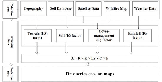
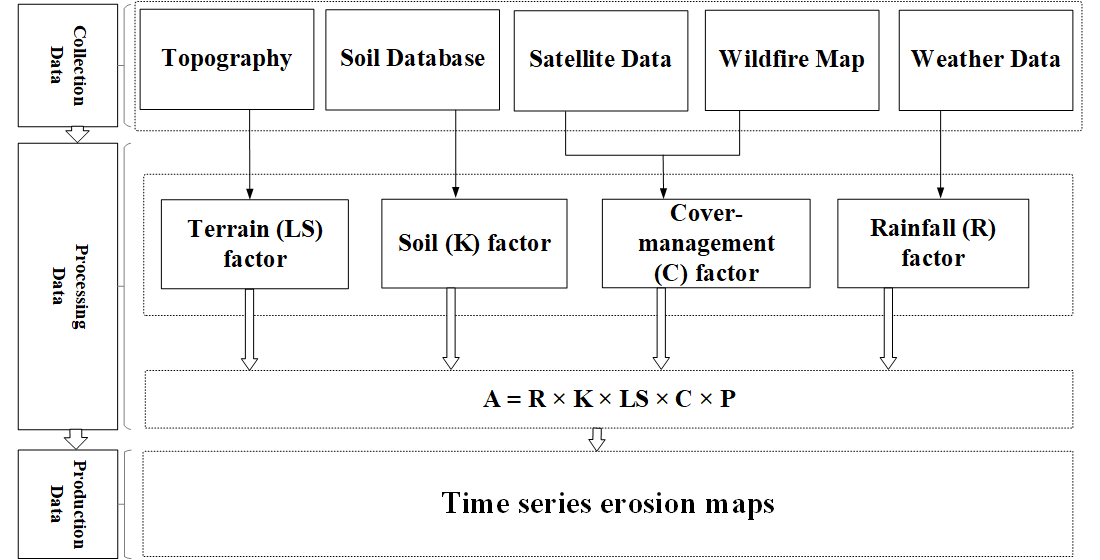
2.3. Event-Based Erosion Modeling

We integrate near real-time weather radar data, remote sensing, Google Earth Engine (GEE), and GIS to obtain and process timely information for hillslope erosion estimation including event-based rainfall erosivity and FVC or the cover-management factor (or C-factor). Along with other erosion factors in relation to soil and topography, we estimate the hillslope erosion at a specific time (Ai) using the modified RUSLE based on [5,9]:

$$A_i=E{I}_{30i} \times C_i \times K_i\times LS\times P_i$$

(1)

where A_i is the computed soil loss per unit area at time i, usually in tons per hectare per time unit (Mg ha⁻¹ time⁻¹); EI_30i is the rainfall–runoff erosivity (R-factor) at time i (usually in MJ mm ha⁻¹ h⁻¹ time⁻¹); K_i is the soil erodibility factor (K-factor, Mg h MJ⁻¹ mm⁻¹), a measure of the susceptibility of soil to erosion; LS is the slope length and steepness factor (LS-factor, dimensionless); C_i is the cover-management factor (C-factor, 0-1 dimensionless); P_i is the erosion control factor (P-factor, set to 1 for this study); i denotes a specific time (i.e., month).

Derivation of the factors required by the RUSLE and its applications in NSW are well described in our previous publications [5,6,7,32,33,34,35]. This study focuses on the recent advancements in weather radar rainfall estimation, satellite estimation of FVC and GEE technology which enable accurate and rapid estimation of some RUSLE factors, specifically for the rainfall erosivity (EI_30i) and cover factors (C_i). In addition to these two dynamic factors, the soil erodibility (K_i) factor was estimated based on [35] using updated soil data (soil texture, structure, permeability, and organic matter) for the SDWC area. Using the DEM derived from Light Detection and Ranging (LiDAR) [31], we calculated the LS-factor for the SDWC area with a 5-m spatial resolution based on [33]. The general procedures are illustrated in Figure 2. All RUSLE factors were resampled to a spatial resolution of 30 m before computing the erosion rates ($A_i$).

2.4. Fractional Vegetation Cover and RUSLE C-Factor Estimation

The RUSLE cover-management factor (C) was estimated from satellite data based on [32] on monthly basis. The satellite data used in this study included MODIS FVC products [25,26,27], Landsat-8 and Sentinel-2 visible, near-infrared (NIR) and shortwave infrared (SWIR) bands, and Google Earth Engine Burnt Area Mapping (GEEBAM) products including normalized burn ratio (NBR) [36]. The multiple data sources are complementary in spatial (10–500 m) and temporal (daily to 16 days) resolutions providing a means for cross validation.

In this study, Sentinel-2 Level-2A surface reflectance (SR) datasets were queried from the GEE data-pool [24]. An automated GEE script (Sen2cor) was developed for data processing and computation including radiometric calibration, geometric calibration, and atmospheric calibration. We produced the Sentinel-2 SR composites for two periods (period 1: July–August 2019, and period 2: January–February 2020), representing the pre-fire season and post-fire season over SDWC.

In addition to the MODIS-derived monthly FVC products at a resolution of 500 m [25,26], the PV fraction (fPV) was estimated based on the modified transformed vegetation index (MTVI) [37] using the NIR and the visible bands as presented in Equation (3). The non-photosynthetic vegetation fraction (fNPV) was estimated from the normalized difference senescent vegetation index (NDSVI) using the red and SWIR (shortwave infrared) reflectance as NPV scattering mostly occurs in the SWIR range [38]. The total cover (TC) was calculated as the summary of fPV and fNPV fraction;

$$f\mathrm{PV}=1.7208\left[1.2\left(R_{NIR}-R_{green}\right)-2.5\left(R_{red}-R_{green}\right)\right]+0.1004$$

(2)

$$f\mathrm{NPV}=0.82\left(R_{SWIR}-R_{red}\right)/\left(R_{SWIR}+R_{red}\right)+0.0753$$

(3)

$$TC=(f\mathrm{PV}+f\mathrm{NPV})/100$$

(4)

The RUSLE cover and management (C) factor were estimated from the TC as:

$$C_j=\exp (-0.799-7.74\times T{C}_j+0.0449\times T{C_j}^2)\times E{I}_j/E{I}_t$$

(5)

where C_j is RUSLE cover-management factor in time j or a given period (e.g., month), TC_j is ground cover (0 to 1) in time j, EI_j is the rainfall erosivity over time j, and EI_t is the total annual rainfall erosivity.

2.5. Rapid Radar Rainfall Data Processing and Storm Event-Based Rainfall Erosivity Estimation

Automated scripts in R (version 3.6), a free software environment for statistical computing and graphics, and GIS (ArcGIS version 10.4) were developed to rapidly process radar Rainfields data and rainfall erosivity estimation based on storm events. The processing included the following steps: i) R scripts were developed for batch processing the radar rainfall data and converting NetCDF to Tiff format; ii) the Tiff datasets were then re-projected to Geographic coordinates so that they match with the other datasets; iii) readjust UTC to AEST (Australian East Standard Time = UTC + 10:00 or 11:00 in daylight saving time); and iv) input to ArcGIS for extraction of rainfall accumulation and further calculations for rainfall erosivity and erosion based on RUSLE and our previous studies [5,6].

The EI30 index is commonly used in RUSLE to predict the impact of rainfall events on soil loss [5,18]. For a single storm event, the EI30 is the value of kinetic energy, E in MJ ha⁻¹, multiplied by the peak 30-min rainfall intensity I₃₀ (mm hr⁻¹). In this study, E is computed from the composite radar Rainfields data in 15-min intervals from BoM following:

$$E={\displaystyle \sum }_{r=1}^N{e}_r{\Delta }{V}_r$$

(6)

$$e_r=0.29[1-0.72\exp (-a\frac{{\Delta }{V}_r}{{\Delta }{t}_r})]$$

(7)

where ∆V_r/∆t_r is the rainfall intensity (mm hr⁻¹), while ∆V_r refers to rainfall amount during that particular period ∆t_r, N is number of 15 min (e.g., N = 2 for 30-min), e_r (MJ ha⁻¹ mm⁻¹) means kinetic energy to single storm event, a is an empirical coefficient. The rainfall intensity for interval 30-min (mm hr⁻¹), I₃₀ is calculated as

$$I_{30}=P_{30}\times 2$$

(8)

P30 is the maximum 30-min rainfall depth (mm); it is multiplied by 2 to convert to an hourly scale. Peak rainfall amount in 30-min intervals was extracted from radar images at every three 15-min intervals. The accumulated EI30 values in a day were compared with the erosivity estimated from a modified daily rainfall erosivity model [5,6].

2.6. Hillslope Erosion Estimation and Risk Scenario Analysis

With all these RUSLE factors, we estimated the hillslope erosion risk for the period of the 2019–2020 fires on a monthly step and on a storm event basis. The pre- and post-fire erosion rates were estimated using FVC estimated from Sentinel-2, Landsat-8, and MODIS, thus providing cross comparison and validation.

The rainfall erosivity percentiles for each month have been calculated from the period 2000 to 2019 to match with the same period of MODIS-derived FVC time series. The GIS (ArcGIS) “rank” function was used to calculate the percentiles. For example, Percentile 95 is 19th rank, percentile 75 is 15th rank, percentile 55 is 11th rank from the 20-year rainfall data. Using these percentiles, we can work out the likely occurrence of an event. For example, if we have a rainfall value in the 90th percentile, this represent the highest 10% erosion risk for this site, or 90% values will be equal to or below this value. The rainfall erosivity percentiles were further spatially interpolated from 5 km to 30 m (using Spline method) to produce higher resolution surfaces in GIS for RUSLE modeling consistent with other factors [29].

Hillslope erosion rates were further estimated and categorized based on these rainfall erosivity percentiles and the C-factor values related to FESM fire severity classes. We first calculated the mean annual rainfall erosivity for the climate normal period (1981–2010) and used as the basis to estimate the various rainfall erosivity percentiles (e.g., 55%, 75%, 95%,) representing rainfall scenarios. The C-factor values were estimated based on the groundcover levels in association with the fire severity classification. For example, Class 1 or low severity with 75% cover, Class 2 or high severity with 50% cover, Class 3 or extreme severity with 25% cover. These combinations of rainfall erosivity and groundcover represent various possible scenarios of rainfall (amount and intensity) and fire severity classes, thus indicating the likely consequences of erosion risk for any given rainfall and fire regime.

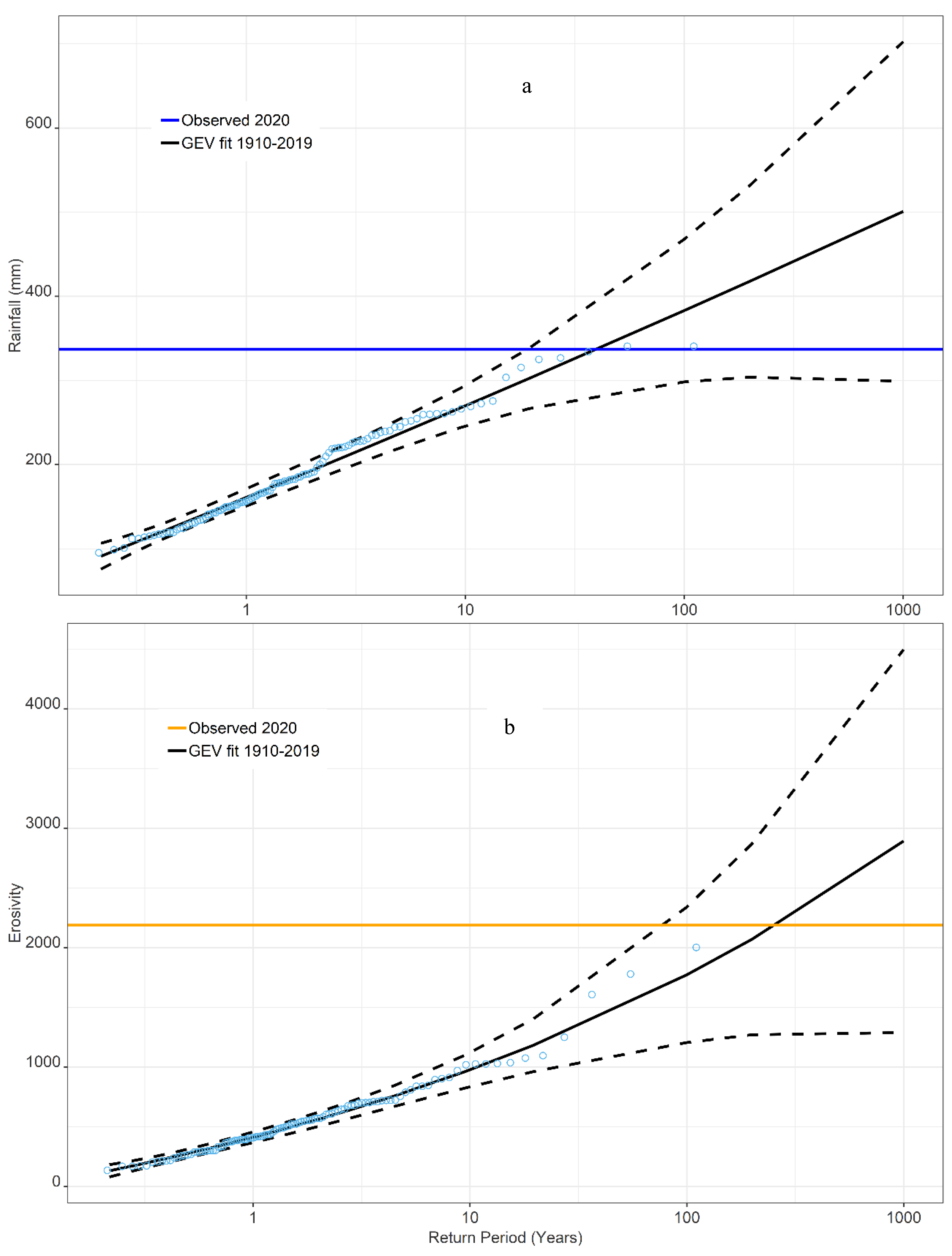
In addition, we also estimated the return period of rainfall and rainfall erosivity for the post-fire storm events by using stationary generalized extreme value (GEV) method [39]. We obtained the annual maxima monthly rainfall, then we fit the GEV to the annual maxima monthly rainfall over the period 1910–2019 using the maximum likelihood method. Then, the parameters of GEV fit were used to plot the return level with the corresponding ±1.96 × standard error for a 95% confidence interval.

2.7. The Normalized Burn Ratio (NBR)

The normalized burn ratio (NBR) and its difference were estimated and used in the GEEBAM program to find out where wildfires in NSW have affected vegetation [36]. GEEBAM used a series of Sentinel-2 images to derive NBR and its difference (dNBR) between the pre-fire and post-fire. NBR is an index designed to highlight burnt areas in large fire zones. The formula is like normalized difference vegetation index (NDVI), except that the formula combines the use of near infrared (NIR) and shortwave infrared (SWIR) wavelengths [40]:

$$NBR=\frac{\left(NIR-SWIR\right)}{\left(NIR+SWIR\right)}$$

(9)

A threshold of dNBR was chosen through visual interpretation to create GEEBAM classes. A higher value of dNBR indicates increased likelihood that the area has burned, while areas with negative dNBR values may indicate regrowth following a fire. GEEBAM was used during the 2019–2020 summer to rapidly predict how severely the tree canopy has burned. It was updated monthly by measuring the change in the color of vegetation after a fire based on NBR. The NBR and fire severity classes were further used in this study to assess the vegetation cover and erosion change before and after the fires.

2.8. Validation of Hillslope Erosion Estimation

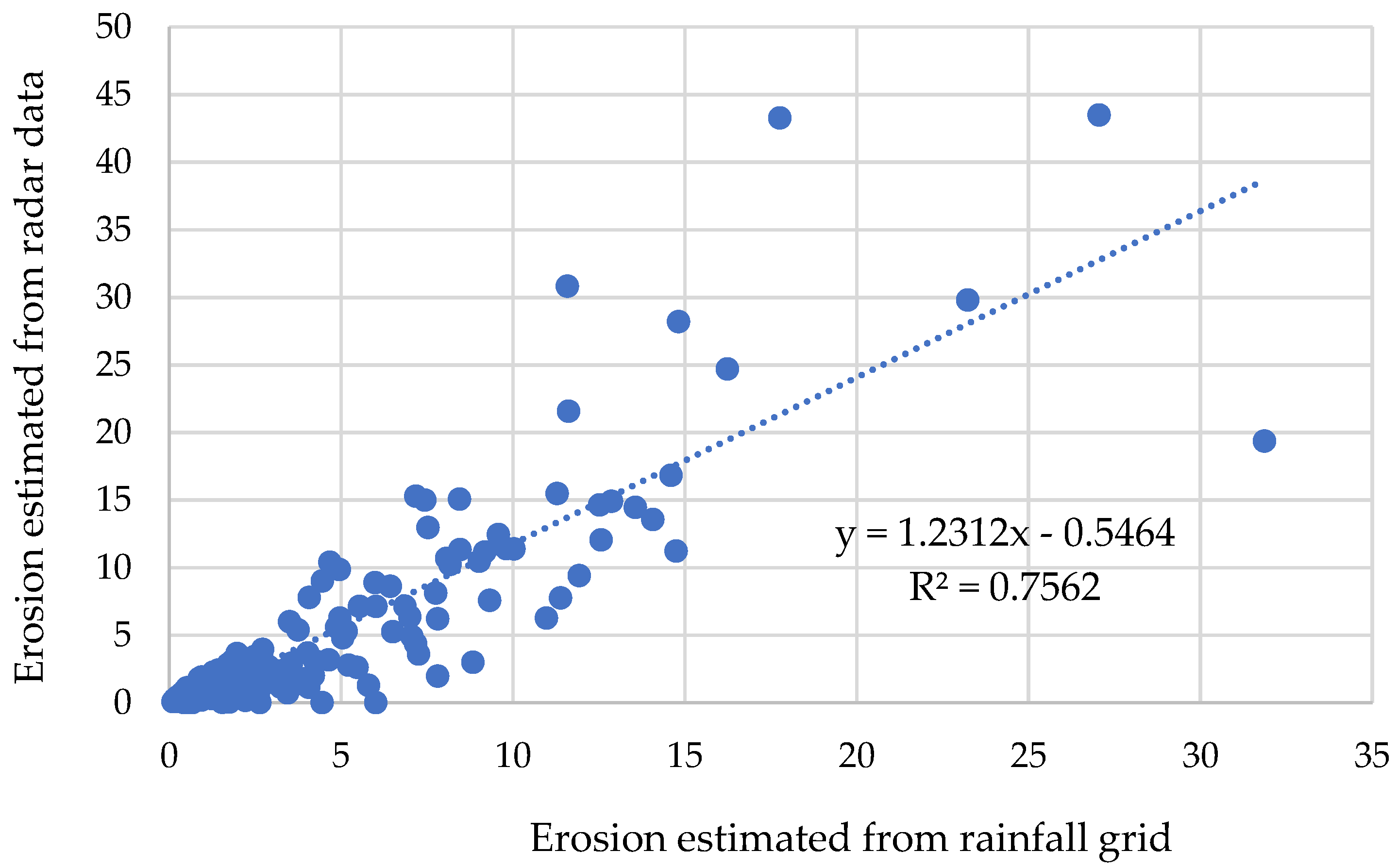
The direct assessment of final erosion results was difficult as it was not possible to carry out field measurements on erosion and sediment immediately after the wildfires and storm events, especially during this Covid-19 pandemic period and the accessibility to the mountainous area. As the K-factor and LS-factor are relatively stable and they were validated in our previous studies, the cross validation in this study was focused on the cover-management and the rainfall erosivity factors (refer Equation (1)). These include: i) The cover-management factor estimated from MODIS, Sentinel-2, and Landsat-8; ii) the rainfall erosivity factor estimated from BoM gridded rainfall and radar rainfall. 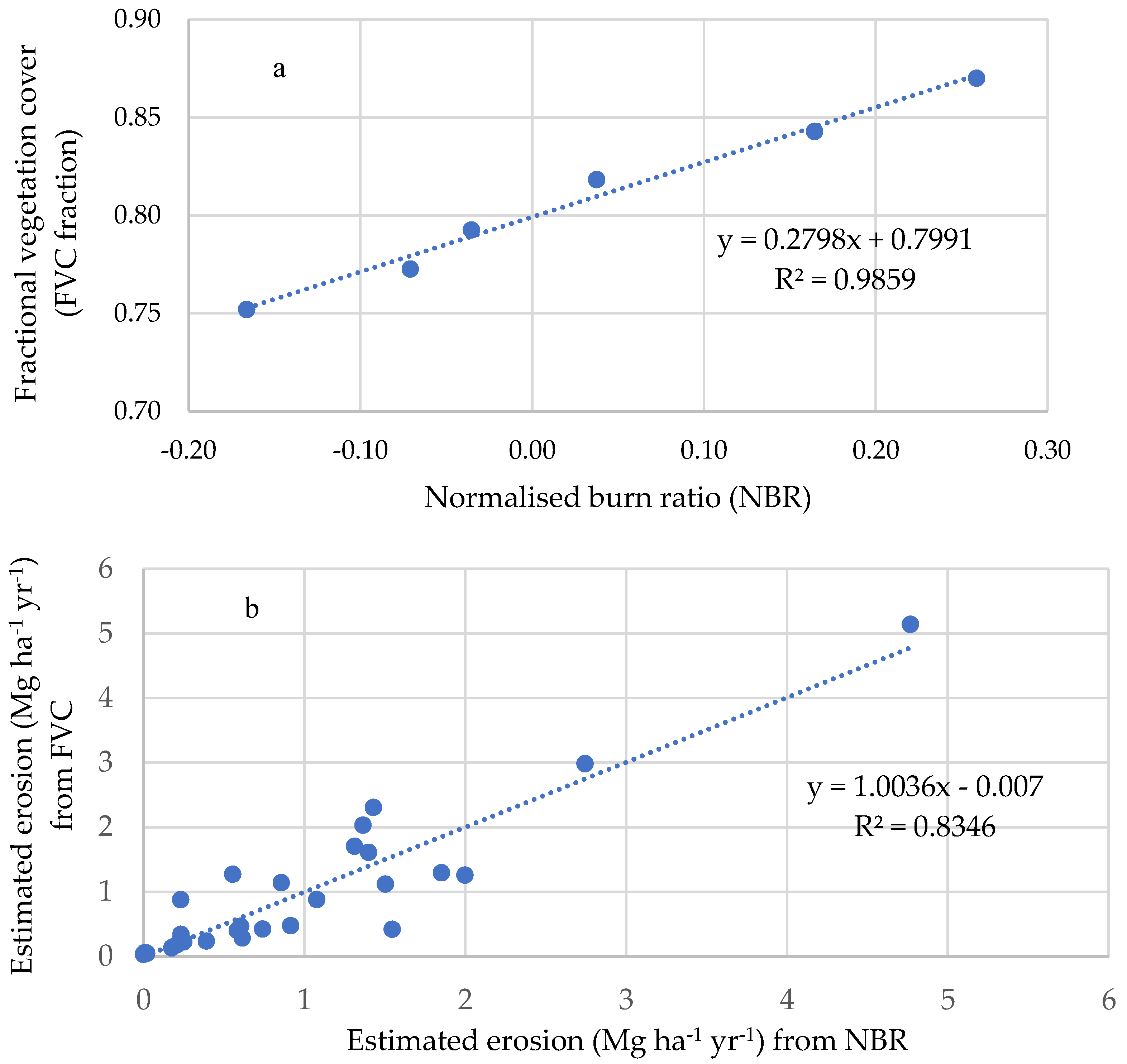The Nash–Sutcliffe model efficiency coefficient (NSE) and relative error were used to assess the relative accuracy and differences [33]. In addition, normalized burn ratio (NBR) as used in GEEBAM was also used to compare FVC (used in RUSLE).

3. Results

3.1. The Temporal Changes of Rainfall, Erosivity and Erosion at SDWC

Based on the historical rainfall records [20], there were only two months over the past 110 years (1910–2020) that had a rainfall amount greater than the post-fire rainfall in February 2020 at SDWC. They were February 1956 and March 1978; both had an average monthly rainfall amount of 341 mm over the SDWC area. Though the rainfall amount (341 mm) was slightly higher than the February 2020 rainfall (337 mm), the rainfall erosivity in February 2020 was estimated the highest (2187.3 MJ mm ha⁻¹ h⁻¹ month⁻¹). This was because the rainfall in February 2020 was more intense as the storm events were concentrated in just several days (6–13 February), thus more erosive. As shown in Figure 3, the return period for the post-fire rainfall in February 2020 was close to a 1-in-40-year event and the rainfall erosivity a 1-in-257-year event based on the GEV-fitted distribution curve for the 1910–2020 climate.

Table 2. Estimated mean monthly erosivity and erosion at Sydney drinking water catchment for the 2019–2020 wildfire period.

Month	FVC (%)	C-factor	Rainfall	Rainfall (Mean)	Erosivity	Erosivity (Mean)	Erosion	Erosion (Mean)
Jul–19	93.5	0.0045	15.9	43	12.0	45.0	0.01	0.04
Aug–19	93	0.0046	22.6	39	16.0	86.5	0.02	0.04
Sep–19	92.5	0.0047	53.1	42	68.7	67.0	0.09	0.05
Oct–19	92.2	0.0048	26.0	53	14.0	92.0	0.02	0.09
Nov–19	90.5	0.0053	18.2	75	12.9	114.7	0.02	0.18
Dec–19	88.8	0.0061	2.6	74	2.0	132.1	0.01	0.17
Jan–20	83.7	0.0081	51.4	78	65.2	167.1	0.16	0.26
Feb–20	86	0.0081	337.2	121	2187.3	332.7	4.88	0.49
Mar–20	90.5	0.007	94.8	88	145.8	105.4	0.24	0.26
Apr–20	93	0.006	53.7	52	58.1	79.2	0.08	0.10
May–20	93	0.006	15.9	37	12.0	68.9	0.07	0.05
Jun–20	93.6	0.006	26	82	13.8	109.5	0.02	0.14

Note: C-factor is unitless; Rainfall in mm month⁻¹; Erosivity in MJ mm ha⁻¹ h⁻¹ month⁻¹; Erosion in Mg ha⁻¹ month⁻¹; the Mean values were calculated for the period 2000–2019.

lists the estimated monthly mean rainfall erosivity and erosion at SDWC for the 2019–2020 wildfire period. The monthly mean values on rainfall, erosivity, and erosion are also listed in the table (mean) for comparison and they were estimated from the recent 20-year rainfall to match at the same period of the available MODIS FVC data (2000–2019). The estimated post-fire erosion rate (4.88 Mg ha⁻¹ month⁻¹) in February 2020 increased more than 30 times compared with the previous months (0.01–0.16 4.88 Mg ha⁻¹ month⁻¹) and about 10 times compared to the mean erosion rate (0.49 Mg ha⁻¹ month⁻¹) in the same month for the period 2000–2019. The average rainfall erosivity value over SDWC in February 2020 was estimated 2187.3 MJ mm ha⁻¹ h⁻¹, exceeding the monthly average value of February by about seven times. It was more than five times higher than what is considered critical in soil erosion (i.e., rainfall erosivity values > 500 MJ mm ha⁻¹ h⁻¹ month⁻¹) [41].

Figure 4 shows the impacts of total vegetation cover and rainfall on erosion at SDWC for the 2019-20 wildfire period. The sharp increase in the erosion rate in February (Mg ha⁻¹ month⁻¹) reflects the combined impacts of wildfire and rainfall on erosion and their relationships.

We further examined the rainfall patterns in February 2020 and found that most erosive rainfall over SDWC area occurred between 6–13 February, accounting for approximately 80% of the total rainfall in that month. With the radar rainfall data at a temporal resolution of 15 min and a spatial resolution of 1000 m, we were able to estimate the EI30 values on hourly and daily basis or storm event basis. Figure 5a shows the estimated daily erosion rate from the radar Rainfields data in January and February 2020. Figure 5b shows an example of the estimated hourly erosion rate from the radar Rainfields data on 9 February, 2020. The radar-based estimation of rainfall erosivity greatly enhanced the temporal and spatial resolutions and potentially more useful for post-fire erosion mitigation.

3.2. The Spatial Variation of Post-Fire Erosion Risk at SDWC

There was great spatial variation in hillslope erosion rates over the SDWC area. Among the 204 drainage units within SDWC, the post-fire erosion rate (February 2020) ranged from 0.1 to 23.8 Mg ha⁻¹ month⁻¹ with a mean value of 4.9 and standard deviation of 4.2 (Mg ha⁻¹ month⁻¹). Figure 6 shows the average monthly erosion risk in January and February 2020 that represents the effect of post-fire storm events on hillslope erosion across the SDWC area. Most of the highest post-fire erosion risk areas appear to be around the Warragamba Dam (Lake Burragorang) including Wild Dog (ID = 193), Lower Kowmung (ID = 99), and Cedar Ck (ID = 33) as shown in the Figure.

Figure 7 further presents the 10 drainage units with the highest erosion rates over the SDWC area after the 2019–2020 wildfires and storm events in February 2020. The erosion rates range from 13.2 Mg ha⁻¹ month⁻¹ in Brogers Ck (ID = 24) to 23.8 Mg ha⁻¹ month⁻¹ in Wild Dog (ID = 193), much higher than the average annual rate in NSW. Linking erosion risk information with these drainage units (the smallest water management units) helps the water management agency (i.e., WaterNSW) to prioritize the monitoring and mitigation actions.

3.3. The Erosion Risk at Different Fire Severity and Erosivity Scenarios

Erosion rates estimated at the high (75 percentile) and extreme (95 percentile) rainfall erosivity scenarios were compared with the average rainfall erosivity in 2000–2019 (the hillslope erosion modeling period). The vegetation cover levels before (July–August 2019) and after (January–February 2020) the 2019–2020 wildfires were estimated from satellite (Sentinel-2 and Landsat-8) derived FVC. It clearly shows the impact of fire severity on hillslope erosion, and the high fire severity class (canopy fully affected) has an erosion risk about two to four times higher compared to other classes. The erosion could increase up to 450% under extreme rainfall erosivity condition for severely burnt areas.

Table 3. Estimated mean erosion rates (Mg ha⁻¹ yr⁻¹) at different fire severity classes and rainfall erosivity scenarios at Sydney drinking water catchment area, and the pre- and post-fire changes.

Fire Severity Class	Estimated Mean Erosion Rates (Mg ha−1 yr−1) and Change%
	Average Rainfall Erosivity			High Rainfall Erosivity		Extreme Rainfall Erosivity
	Pre-Fire	Post-Fire	Change% (%)	Post-Fire	Change%	Post-Fire	Change%
Low	6.0	9.2	52	10.2	68	17.5	190
Moderate	6.1	10.8	76	12.6	105	20.4	232
High	4.5	8.6	91	10.2	126	16.0	254
Extreme	3.5	10.6	202	12.5	255	19.3	448

summarized the estimated erosion rates under different fire severity classes and rainfall scenarios. Unlike the relative change (%), the actual erosion rates are not always positively correlated to the fire severity classes because of the impacts of other factors such as rainfall, terrain, and soil (refer Equation (1)).

3.4. Cross Validation and Comparison of Results

Using the relationship between NBR and FVC we estimated the erosion risk directly from NBR using the established methods as presented above, the coefficient of determination (R²) from the erosion estimates between FVC and NBR reached 0.8346 (Figure 8). It implies that the commonly used NBR index in wildfire studies can be used as a substitute for FVC to estimate the C-factor values and the erosion rates along with other RUSLE factors.

Figure 9 compares the rainfall erosivity and the final erosion estimation from the BoM daily rainfall gridded data (5 km) and the radar Rainfields data (15 min, 1 km). Though the source datasets are very different in resolution and measurement, there is a high correlation between them (R² = 0.7562), implying that the radar Rainfileds data can be directly used in estimating erosivity.

4. Discussion

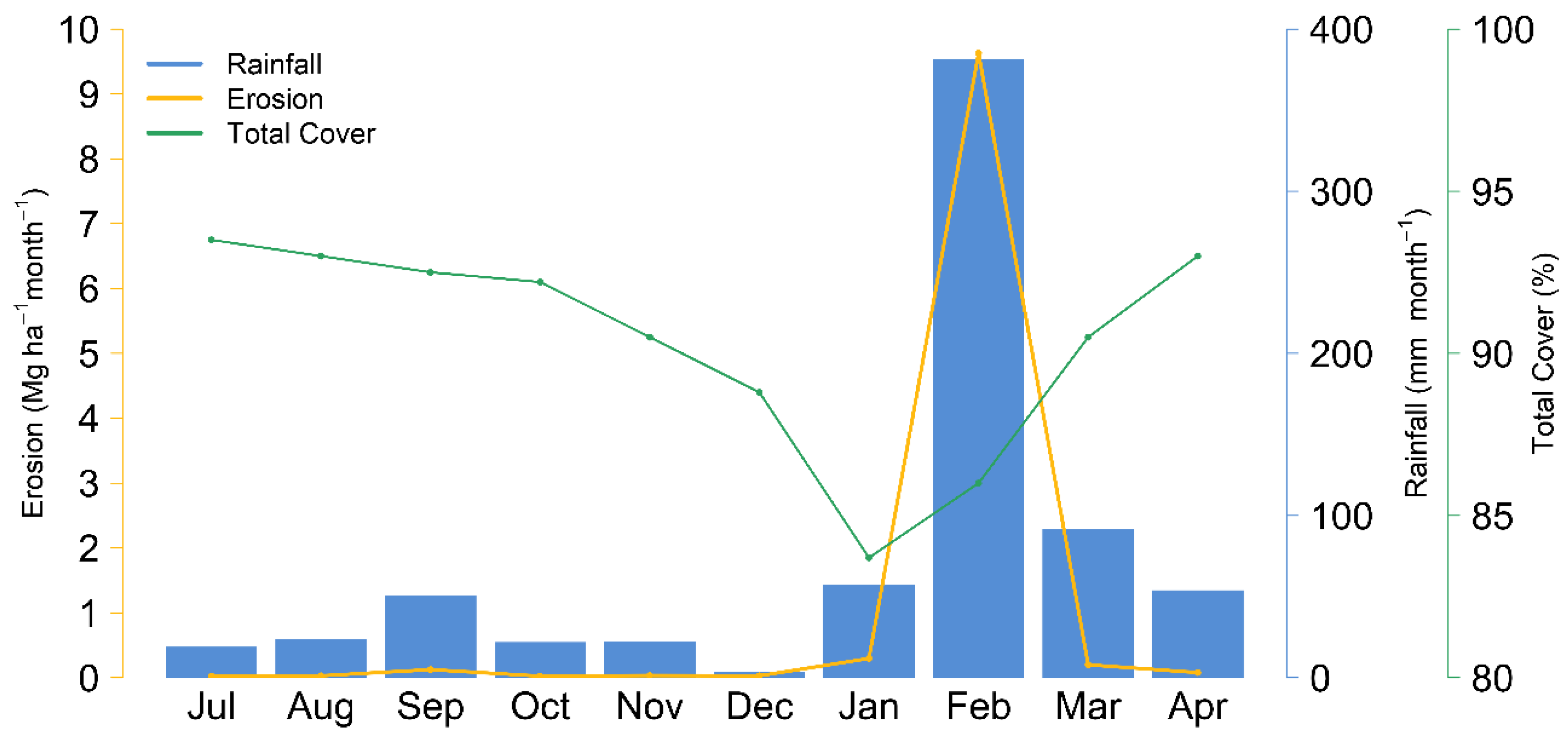
Vegetation cover (or C-factor) and rainfall (or R-factor) are the two dominant factors affecting the post-fire hillslope erosion. Vegetation cover, which is important in reducing the impact of rainfall, was not significantly lower (about 10%) after the wildfire based on the monthly FVC products [25,26,27]. Over 80% of the soil surface was still covered by either PV or NPV, both can protect soil from erosion. This agrees well with the study in another national park in Australia [40,41].

Compared to the mean values in February for all years (2000–2020), C-factor value only increased 1.5 times (due to wildfire) but the rainfall erosivity increased about 7 times in February 2020 across the SDWC area. This suggests that rainfall has a far larger impact than groundcover factor, on hillslope erosion after wildfires. This is in line with a similar study in the Blue Mountains catchment using the eWater toolkit (Source) model which reported six times higher sediment load at the downstream outlet after extreme wildfire in 2001 [42]. The post-fire soil erosion is mainly limited by rainfall erosivity which agrees with similar studies [43,44,45].

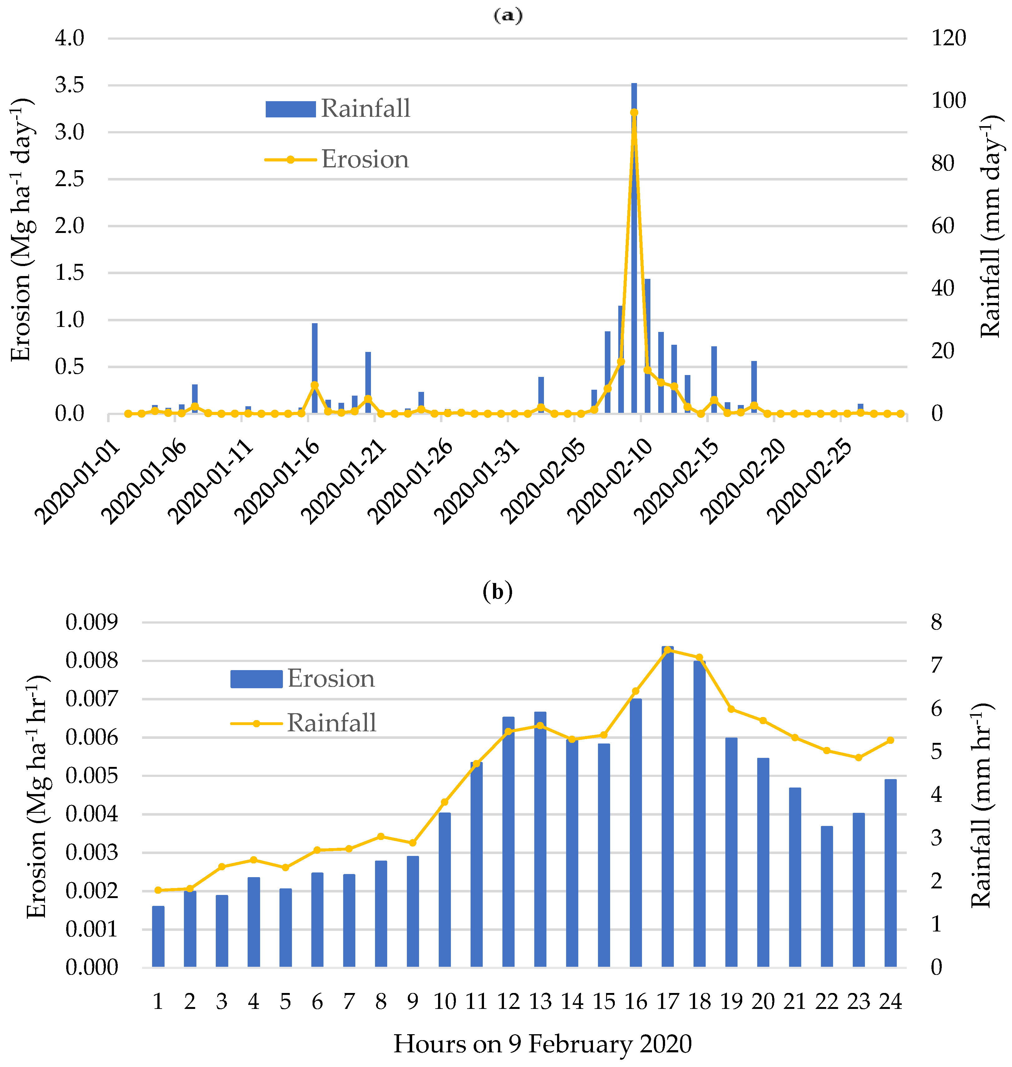
There was a prolonged dry period before the 2019–2020 wildfires with less than 300 mm rainfall over the SDWC area for 10 months from April 2019 to January 2020, leading to large quantities of fuel loads. In February 2020 the rainfall amount reached 337 mm month⁻¹, with several intense storm events between 6–13 February. The severe hillslope erosion at SDWC was mainly caused by these extreme rainfall events in February 2020. For example, the erosion rate on a single day (9 February 2020) reached 3.2 (Mg ha⁻¹ day⁻¹) which contributed to 65% of the total monthly erosion (4.9 Mg ha⁻¹ Month⁻¹) in February 2020.

Despite the increased erosion risk, WaterNSW successfully maintained the supply of safe water to the treatment plants, by proactively managing the water supply system configuration (through sources selection and offtake depth changes) preventing the inflows from the fire-impacted catchment entering the supply during these storm events.

Soil erodibility (K) and slope-steepness (LS) factors are relatively stable compared to the dynamic C-factor and R-factor. Wildfires may alter the soil properties including soil structure, texture, permeability, and soil organic carbon which are all related to the K-factor as discussed in one of our previous studies [46]. The extent of fire effects on these soil properties depends on fire intensity, fire severity, and fire frequency [47] which is complicated and beyond the scope of this study.

The terrain factor also contributed significantly to the post-fire erosion. SWDC area has a rugged terrain compared with many other parts of NSW. The mean slope is about 17% over the SDWC area, and 29% in the Warragamba Dam area, much higher than the state average (6%). Because of the steep terrain, the mean RUSLE LS-factor value at SDWC is 4.7 which is about 2.6 time higher than the State average (1.8). The LS-factor value at the Warragamba Dam area is even higher (7.2) which is about 4 times of the State average. This implies that the erosion risk at our drinking water catchments are likely to be 2.6–4 times higher than the rest of the State regardless of other erosion factors. This also implies the importance of maintaining good vegetation cover and erosion control practices in the drinking water catchment area.

RUSLE, when appropriately used, can produce meaningful information on relative hillslope erosion risk at a given time. The event-based rainfall erosivity estimation relies on the availability of high-resolution rainfall data. The weather radar Rainfield data (15-min, 1 km) are adequate for estimating EI30 index at daily or sub-daily scale. Such data sets will be increasingly important because of the higher likelihood of intense storm events and fire frequency under the changing climate with warmer and drier conditions.

In a GEE environment, various remote sensing data can be searched and used to estimate the FVC and RUSLE C-factor. The widely used NBR in fire severity mapping and FVC has close correlation and can be used as a surrogate to FVC for C-factor estimation in erosion modeling.

As the erosion model has been applied at such high spatial (5–30 m) and temporal (daily or hourly) resolutions, the impacts of fires on soil erosion can be explored at finer landscape scales including individual hydrological catchments, drainage units, or even paddocks. This helps to locate the high erosion risk areas or sediment sources to assist prioritized management practices. Accurate and effective decision-making is best enabled by linking with detailed and timely information on erosion to identify the impacts of rain events after the fires.

However, process-based studies to understand the factors controlling surface runoff and erosion, particularly in relation to aspects of the fire regime are still required to precisely predict the sediment transport and deposition, especially in the waterways.

5. Conclusions

This study developed an innovative yet practical approach for rapid assessment of post-fire hillslope erosion risk using weather radar, remote sensing, GEE, and GIS. The automated scripts running in ArcGIS and GEE allow rapid processing of time-series and event-based spatial data including satellite and weather radar images to estimate the erosion risk for the 2019–2020 wildfires at SDWC.

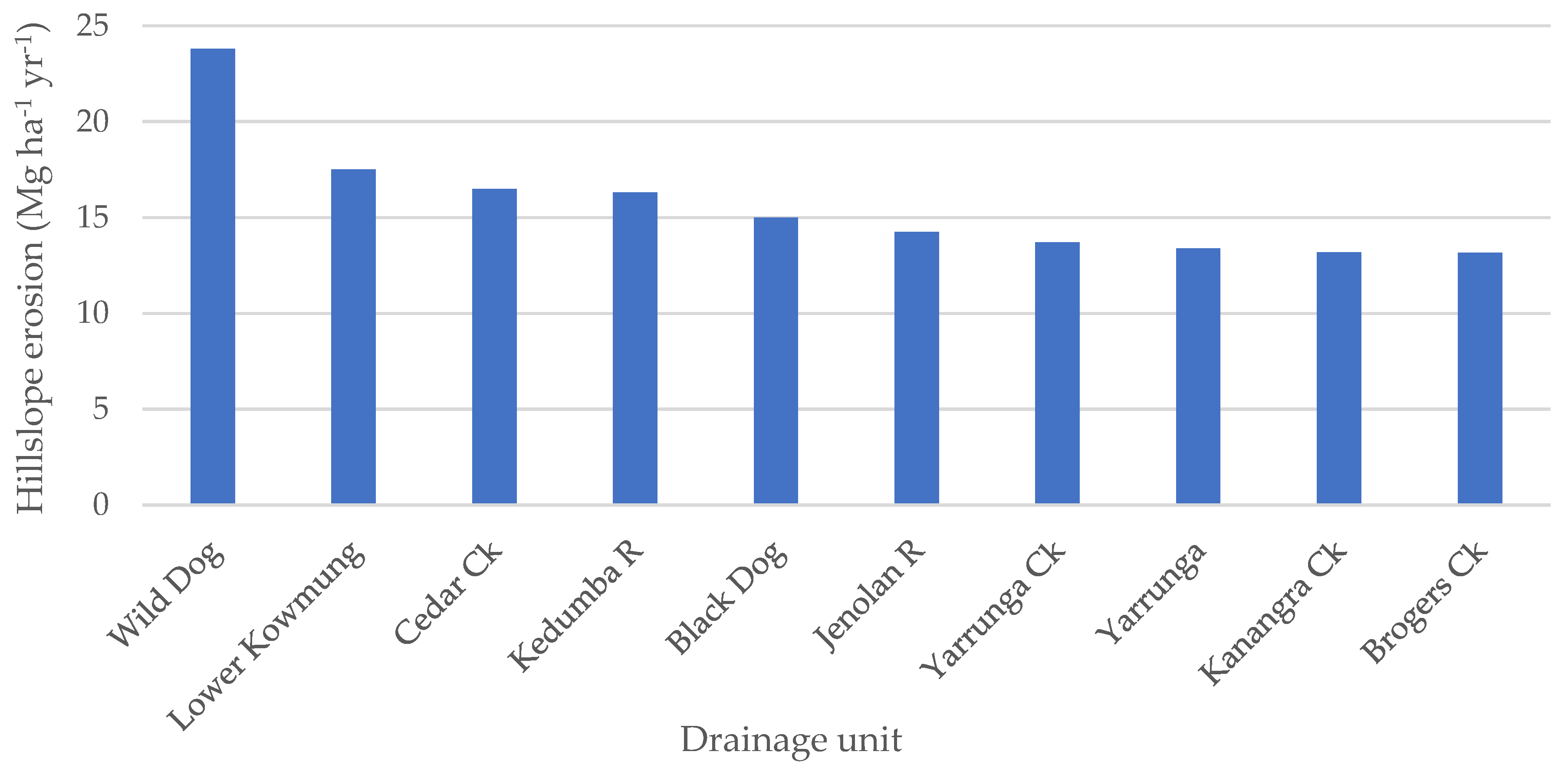
This study was the first attempt to precisely estimate where and when high erosion risk is likely to occur at daily and/or hourly steps after severe wildland fires across large drinking water catchments, allowing for more accurate estimation of event-based erosion. With these timely estimates of rainfall erosivity and C-factor, along with the existing datasets on soil erodibility and slope-steepness, we were able to deliver rapid assessment of the post-fire hillslope erosion risk and link it with fire severity. These continuous and consistent estimates of erosion rates were used to analyze the erosion risk before and after the 2019–2020 wildfires and the subsequent impacts of rainfall on erosion rates. With these time series datasets, we identified the locations and times of the highest erosion risk. The sub-catchments near Warragamba Dam have the highest erosion risk because of the bushfires and rainfall events.

The rainfall erosivity is the dominant factor affecting hillslope erosion after severe wildfires over the SDWC area. Severe erosion events are often caused by short but intense storm events such as the case in February 2020. High temporal rainfall data are essential in rainfall erosivity modeling. Weather radar Rainfields data are adequate for erosivity or EI30 estimation at catchment and regional scales.

Field observations and measurements of soil erosion are necessary for model validation and improvement. Other relevant water quality models (such as Source developed by eWater Australia) may be used jointly to validate the modeling accuracy and predict likely pollution risk and delivery to the river or lake system after severe wildfires [48]. Over the next two-years we plan to collect more field data on erosion level, ground cover, land management activity, slope and slope length will be gathered along a set of transects at selected trial catchments for further calibration and validation of methods. A hillslope sediment erosion trap network, consisting of moderate and low burn severity, prescribed burn, rainfall event-based, and control sites are planned to be installed at SDWC sub-catchments along with the water quality stations, and maintained by Water NSW. The goal of the traps is to collect post-fire and unburnt erosion rates to validate model estimates. This will help further calibrate and improve the erosion model and link the estimated erosion rates with sediment transport and water quality downstream. The methodology, once fully validated, will be extended to other areas and wildfire events to provide timely and accurate information on erosion water quality immediately after wildfires.