Beyond Measurement: Extracting Vegetation Height from High Resolution Imagery with Deep Learning


Abstract
1. Introduction
2. Materials and Methods
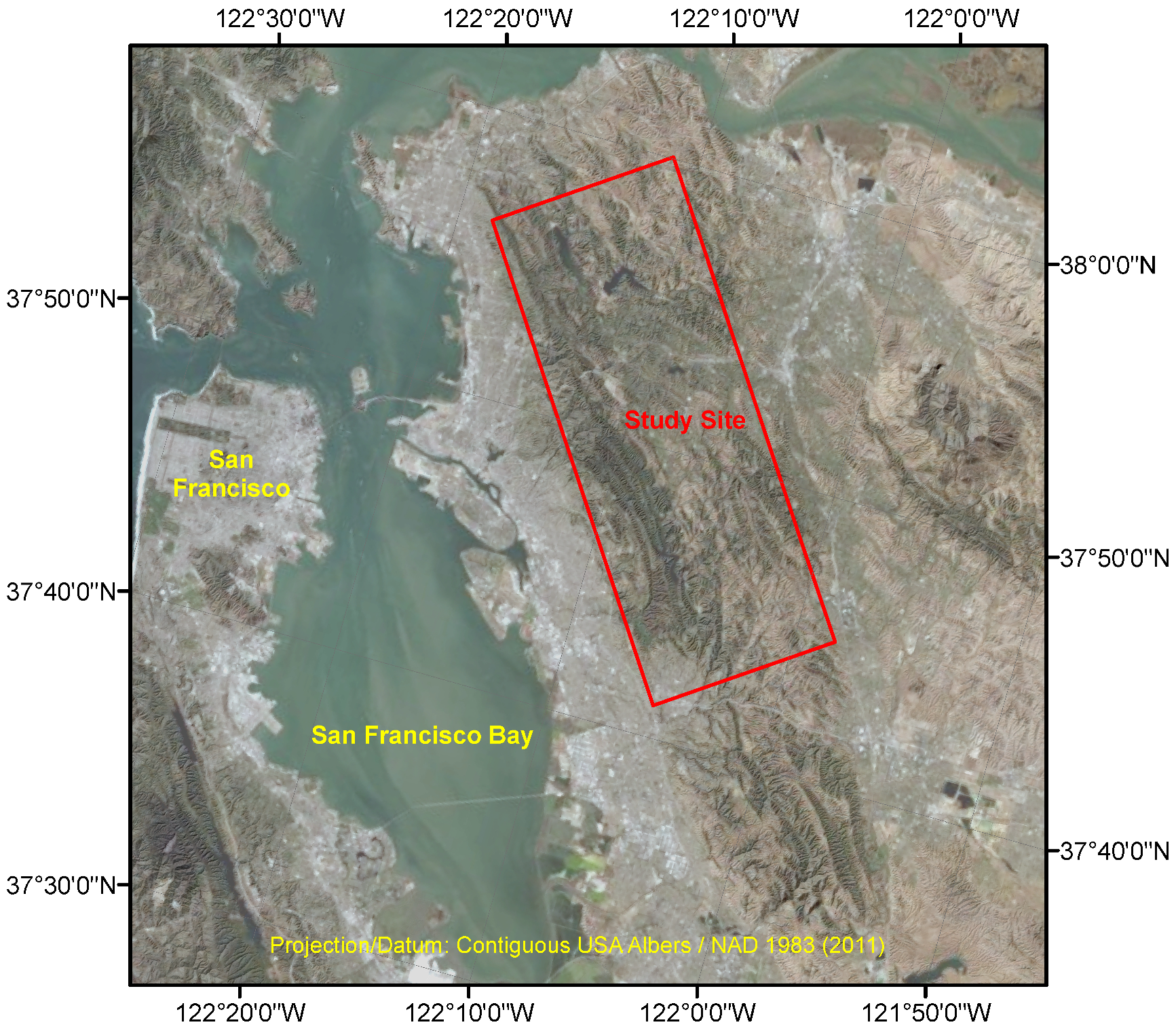
2.1. Study Site
2.2. Data Features and Processing
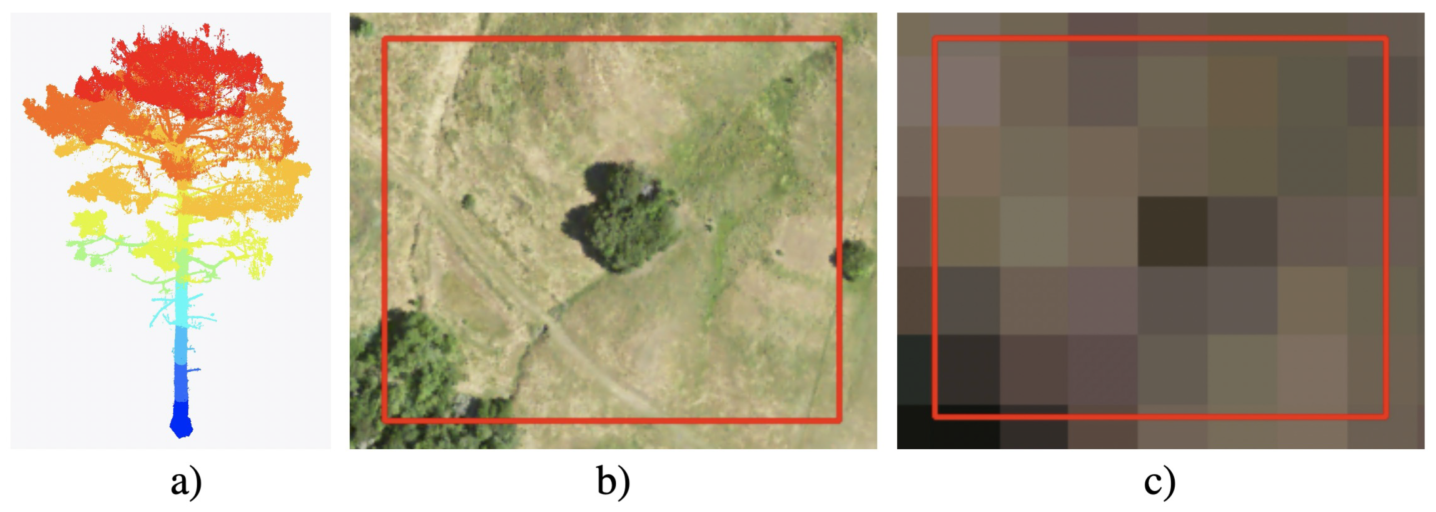
2.2.1. Visual Data
2.2.2. Terrain Data
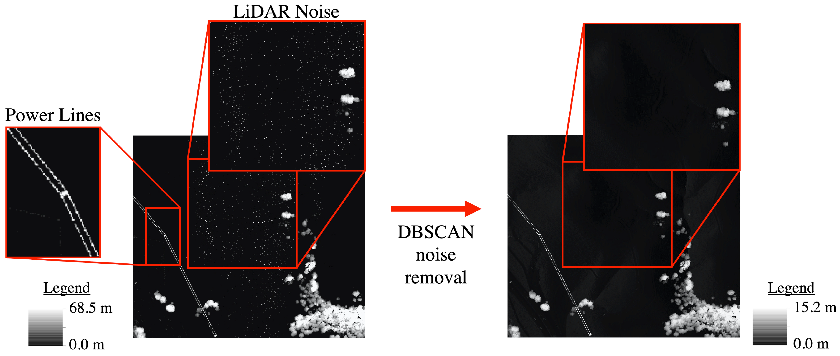
2.2.3. LiDAR Derived Dataset Labels
2.3. Deep Learning Background
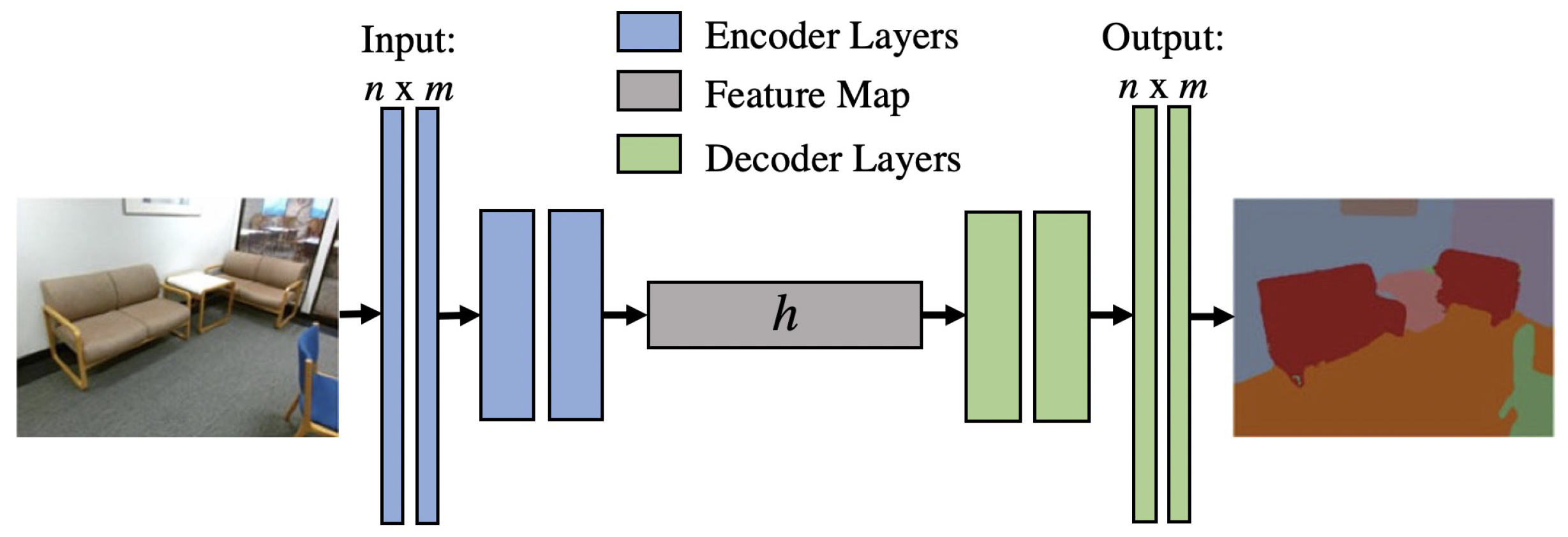
2.4. U-NET
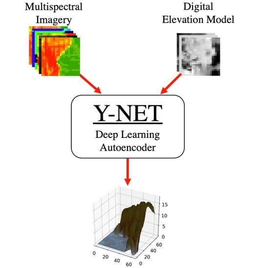
2.5. Our Model: Y-NET
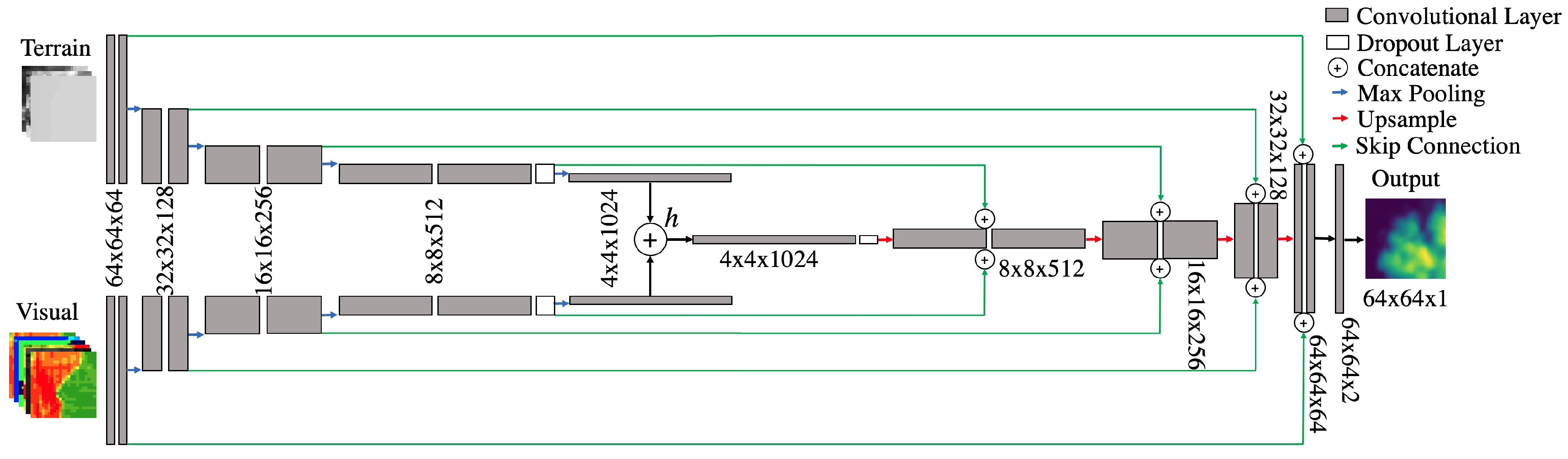
2.5.1. Architecture and Training
2.5.2. Motivation and Inspiration
2.5.3. Workflow & Implementation
2.6. Evaluation
3. Results
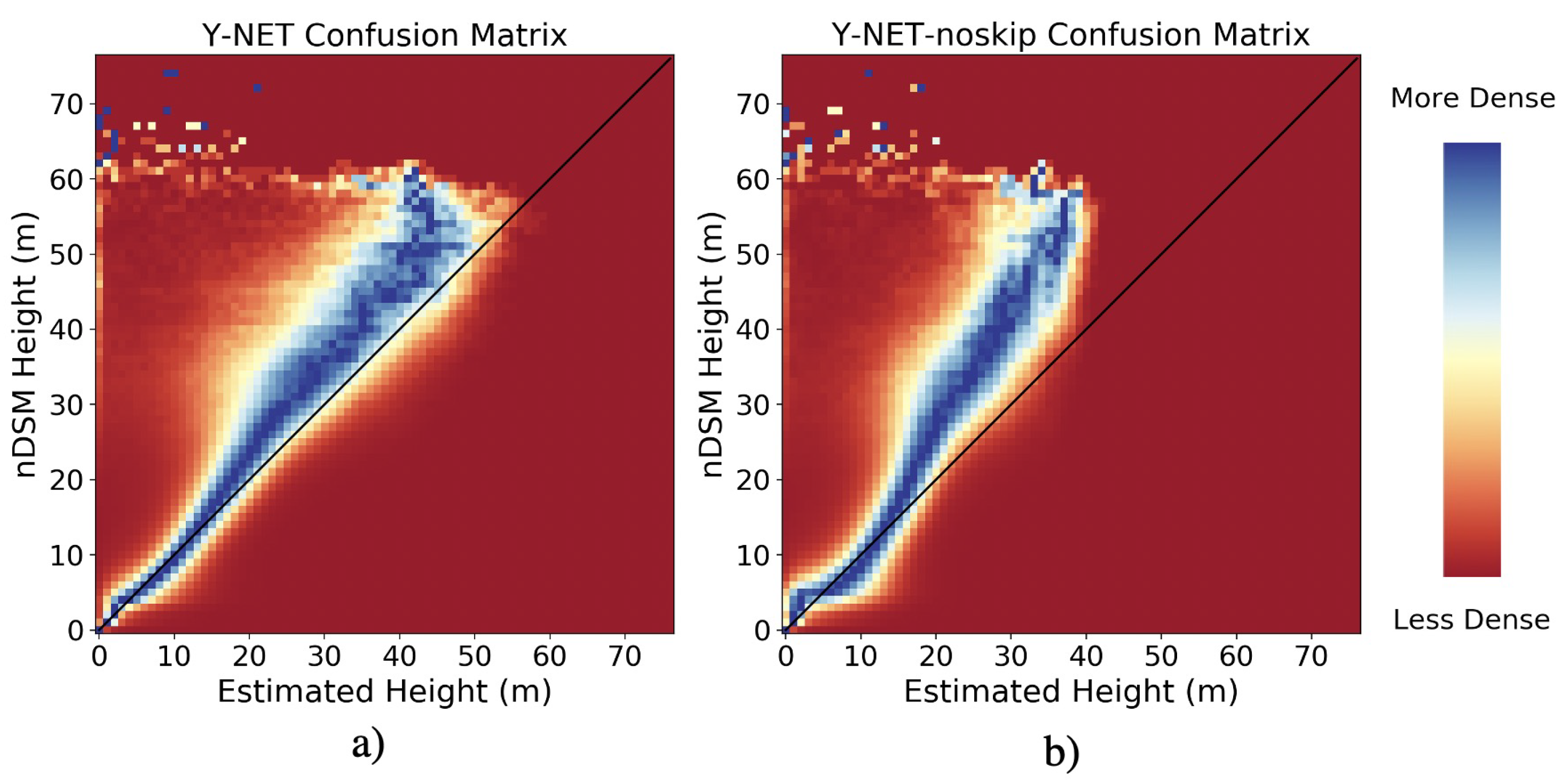
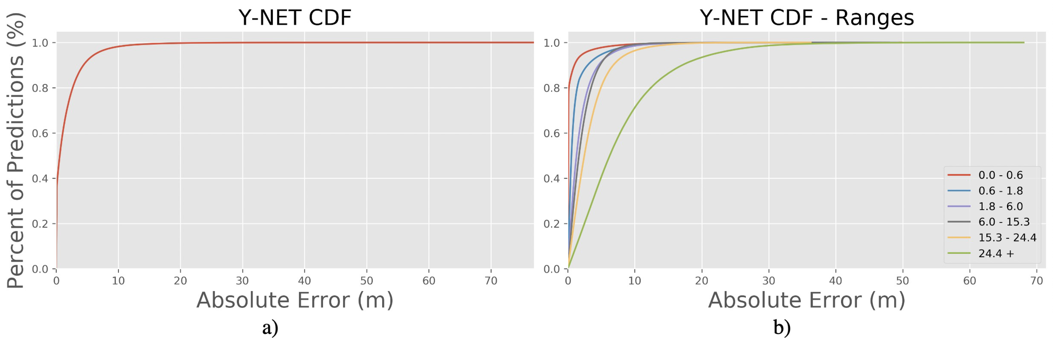
3.1. Statistical Results
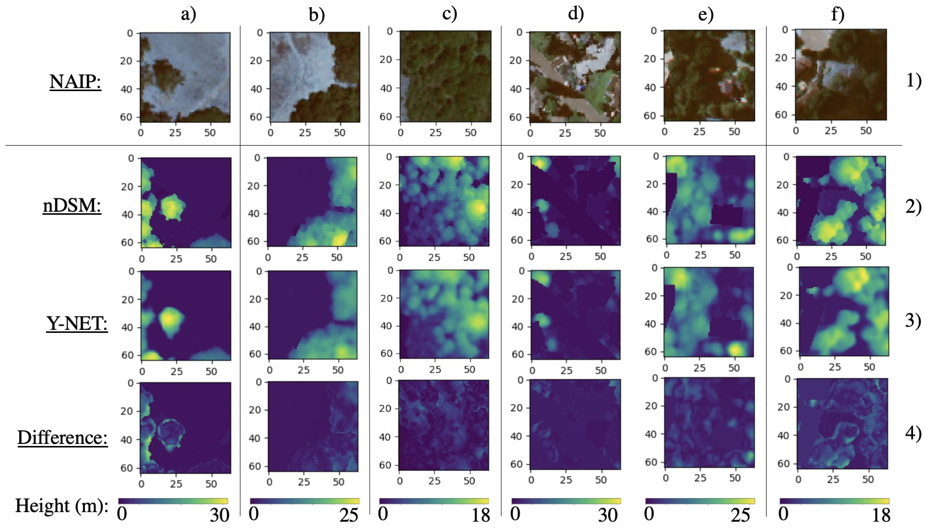
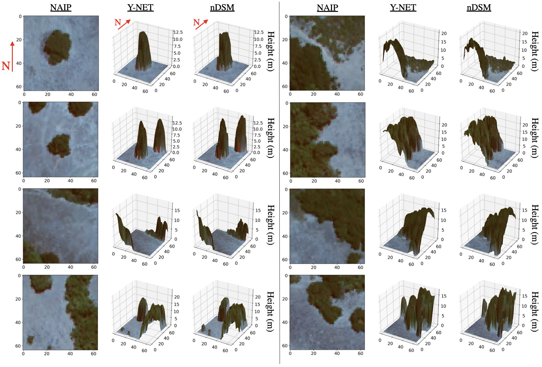
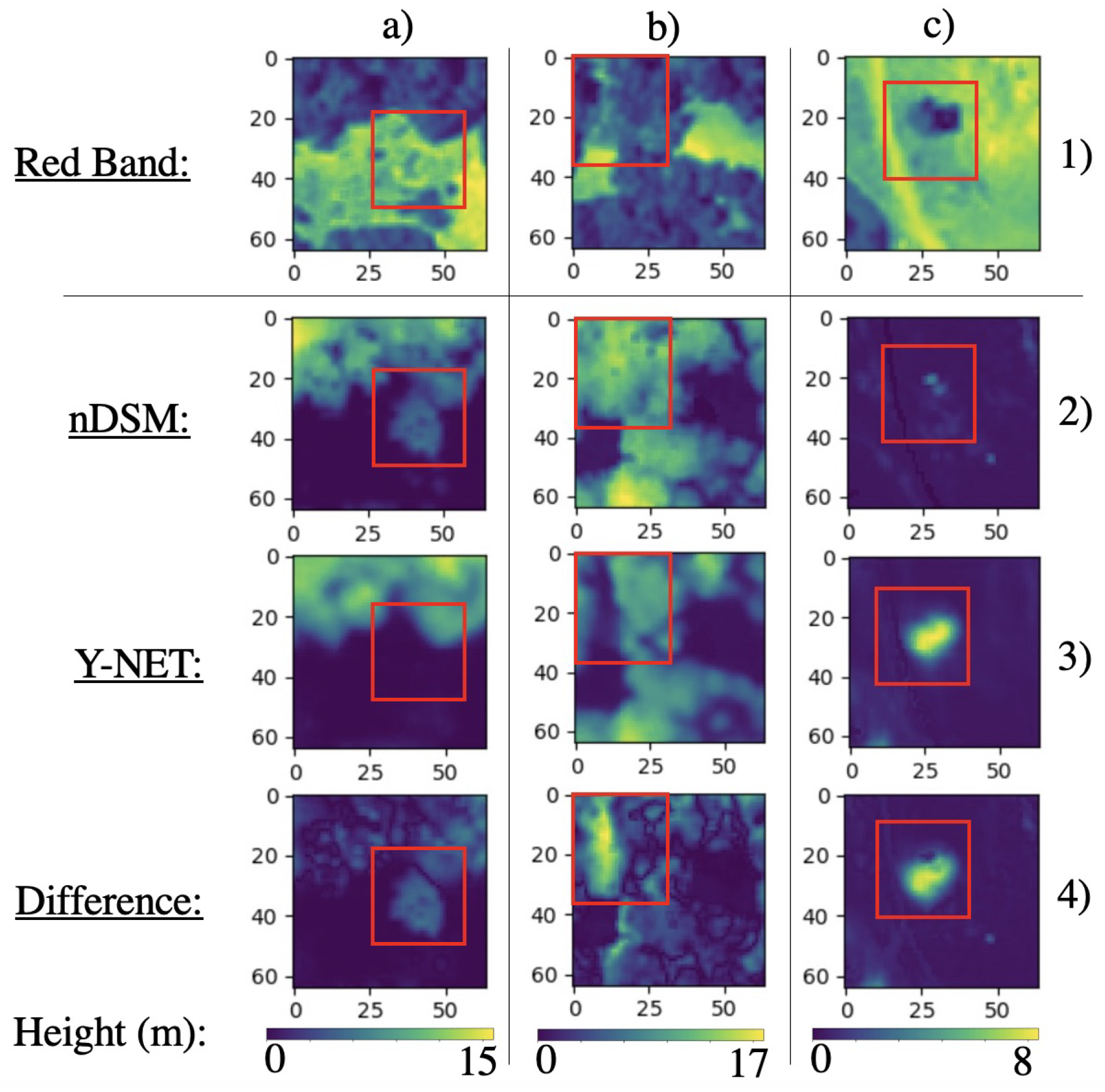
3.2. Visual Results
4. Discussion
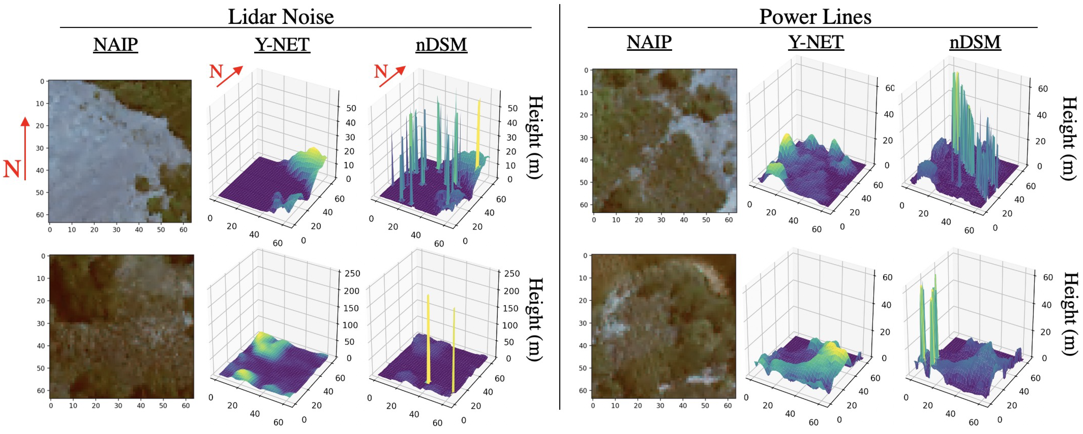
4.1. Long CDF Tails
4.2. Vegetation Mitigation and Growth
4.3. Impact
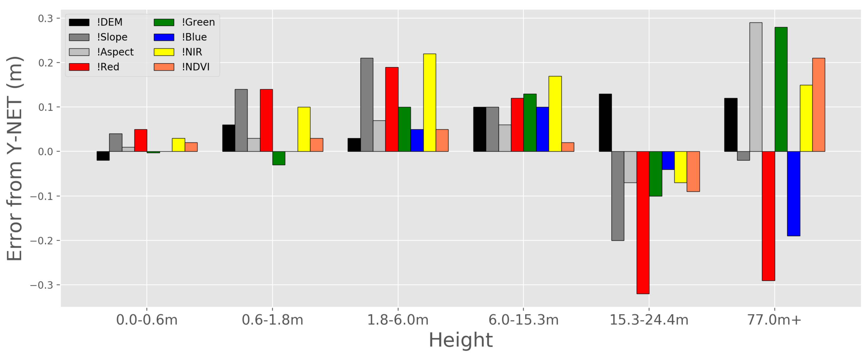
4.4. Input Feature Ablation Study
4.5. Future Work
5. Conclusions
Author Contributions
Funding
Acknowledgments
Conflicts of Interest
References
- Franklin, S.E. Remote Sensing for Sustainable Forest Management; Lewis Publishers: Boca Raton, FL, USA, 2001. [Google Scholar]
- Skole, D.; Tucker, C. Tropical Deforestation and Habitat Fragmentation in the Amazon: Satellite Data from 1978 to 1988. Science 1993, 260, 1905–1910. [Google Scholar] [CrossRef] [PubMed]
- Russell, W.H.; McBride, J.R. Landscape scale vegetation-type conversion and fire hazard in the San Francisco bay area open spaces. Landsc. Urban Plan. 2003, 64, 201–208. [Google Scholar] [CrossRef]
- Keeley, J.E. Fire history of the San Francisco East Bay region and implications for landscape patterns. Int. J. Wildland Fire 2005, 14, 285–296. [Google Scholar] [CrossRef]
- Westerling, A.L.; Hidalgo, H.G.; Cayan, D.R.; Swetnam, T.W. Warming and Earlier Spring Increase Western U.S. Forest Wildfire Activity. Science 2006, 313, 940–943. [Google Scholar] [CrossRef]
- Flores, L.; Martinez, L. Land Cover Estimation in Small Areas Using Ground Survey and Remote Sensing. Remote Sens. Environ. 2000, 74, 240–248. [Google Scholar] [CrossRef]
- Mikita, T.; Janata, P.; Surovy, P. Forest Stand Inventory Based on Combined Aerial and Terrestrial Close-Range Photogrammetry. Forests 2016, 7, 165. [Google Scholar] [CrossRef]
- Solberg, S.; Astrup, R.; Gobakken, T.; Næsset, E.; Weydahl, D.J. Estimating spruce and pine biomass with interferometric X-band SAR. Remote Sens. Environ. 2010, 114, 2353–2360. [Google Scholar] [CrossRef]
- Greaves, H.E.; Vierling, L.A.; Eitel, J.U.; Boelman, N.T.; Magney, T.S.; Prager, C.M.; Griffin, K.L. Estimating aboveground biomass and leaf area of low-stature Arctic shrubs with terrestrial LiDAR. Remote Sens. Environ. 2015, 164, 26–35. [Google Scholar] [CrossRef]
- Nikolakopoulos, K.G.; Soura, K.; Koukouvelas, I.K.; Argyropoulos, N.G. UAV vs. classical aerial photogrammetry for archaeological studies. J. Archaeol. Sci. Rep. 2017, 14, 758–773. [Google Scholar] [CrossRef]
- Solberg, S.; Astrup, R.; Bollandsås, O.M.; Næsset, E.; Weydahl, D.J. Deriving forest monitoring variables from X-band InSAR SRTM height. Can. J. Remote Sens. 2010, 36, 68–79. [Google Scholar] [CrossRef]
- Schuster, C.; Ali, I.; Lohmann, P.; Frick, A.; Forster, M.; Kleinschmit, B. Towards Detecting Swath Events in TerraSAR-X Time Series to Establish NATURA 2000 Grassland Habitat Swath Management as Monitoring Parameter. Remote Sens. 2011, 3, 1308–1322. [Google Scholar] [CrossRef]
- Lopez-Sanchez, J.M.; Ballester-Berman, J.D.; Hajnsek, I. First Results of Rice Monitoring Practices in Spain by Means of Time Series of TerraSAR-X Dual-Pol Images. IEEE J. Sel. Top. Appl. Earth Obs. Remote Sens. 2011, 4, 412–422. [Google Scholar] [CrossRef]
- Perko, R.; Raggam, H.; Deutscher, J.; Gutjahr, K.; Schardt, M. Forest Assessment Using High Resolution SAR Data in X-Band. Remote Sens. 2011, 3, 792–815. [Google Scholar] [CrossRef]
- Hyde, P.; Dubayah, R.; Walker, W.; Blair, J.; Hofton, M.; Hunsaker, C. Mapping forest structure for wildlife habitat analysis using multi-sensor (LiDAR, SAR/InSAR, ETM+, Quickbird) synergy. Remote Sens. Environ. 2006, 102, 63–73. [Google Scholar] [CrossRef]
- Maltamo, M.; Malinen, J.; Packalén, P.; Suvanto, A.; Kangas, J. Nonparametric estimation of stem volume using airborne laser scanning, aerial photography, and stand-register data. Can. J. Remote Sens. 2006, 36, 426–436. [Google Scholar] [CrossRef]
- Radke, J.D.; Biging, G.S.; Roberts, K.; Schmidt-Poolman, M.; Foster, H.; Roe, E.; Ju, Y.; Lindbergh, S.; Beach, T.; Maier, L.; et al. Assessing Extreme Weather-Related Vulnerability and Identifying Resilience Options for California’s Interdependent Transportation Fuel Sector; California’s Fourth Climate Change Assessment, California Energy Commission: Sacramento, CA, USA, 2018; Publication Number: CCCA4-CEC-2018-012. [Google Scholar]
- Buckley, J. Isebrands, T.S. Practical field methods of estimating canopy cover, PAR, and LAI in Michigan Oak and pine stands. North. J. Appl. For. 1999, 16, 25–32. [Google Scholar] [CrossRef]
- Digital Globe. Available online: https://www.digitalglobe.com (accessed on 29 September 2020).
- Planet. Available online: https://www.planet.com (accessed on 29 September 2020).
- United States Geological Survey. Available online: https://www.usgs.gov (accessed on 29 September 2020).
- Stojanova, D.; Panov, P.; Gjorgjioski, V.; Kobler, A.; Džeroski, S. Estimating Vegetation Height and Canopy Cover from Remotely Sensed Data with Machine Learning. Ecol. Inform. 2010, 5, 256–266. [Google Scholar] [CrossRef]
- Gu, C.; Clevers, J.G.P.W.; Liu, X.; Tian, X.; Li, Z.; Li, Z. Predicting Forest Height using the GOST, Landsat 7 ETM+, and Airborne LiDAR for Sloping Terrains in the Greater Khingan Mountains of China. ISPRS 2018, 137, 97–111. [Google Scholar] [CrossRef]
- Dżeroski, S.; Kobler, A.; Gjorgjioski, V.; Panov, P. Predicting forest stand height and canopy cover from Landsat and Lidar data using data mining techniques. In Proceedings of the Poster Presentation at Second NASA Data Mining Workshop: Issues and Applications in Earth Science, Pasadena, CA, USA, 23–24 May 2006. [Google Scholar]
- Radke, D.; Hessler, A.; Ellsworth, D. FireCast: Leveraging Deep Learning to Predict Wildfire Spread. In Proceedings of the Twenty-Eighth International Joint Conference on Artificial Intelligence, IJCAI-19, Macao, Macao, 10–16 August 2019; pp. 4575–4581. [Google Scholar] [CrossRef]
- Finney, M.A. FARSITE: Fire Area Simulator—Model Development and Evaluation; US Forest Service: Missoula, MT, USA, 1998.
- National Agriculture Imagery Program. Available online: https://www.sciencebase.gov/catalog/item/51355312e4b0e1603e4fed62 (accessed on 29 September 2020).
- Gov. Newson Visits East Bay Hills to Highlight Wildfire Danger, Prevention Efforts. Available online: https://www.mercurynews.com/2019/04/23/gov-newsom-visits-east-bay-hills-to-highlight-wildfire-danger-prevention-efforts/ (accessed on 29 September 2020).
- Moraga-Orinda Fire District Awarded Major State Wildfire Prevention Grant. Available online: https://www.dailydispatch.com/StateNews/CA/2019/March/20/MoragaOrinda.Fire.District.awarded.major.state.wildfire.prevention.grant.aspx (accessed on 29 September 2020).
- McBride, J.R.; Kent, J. The failute of planning to address the urban interface and intermix fire-hazard problems in the San Francisco Bay Area. Int. J. Wildland Fire 2019, 28, 1–3. [Google Scholar] [CrossRef]
- Luo, S.; Wang, C.; Pan, F.; Xi, X.; Li, G.; Nie, S.; Xia, S. Estimation of wetland vegetation height and leaf area index using airborne laser scanning data. Ecol. Indic. 2015, 48, 550–559. [Google Scholar] [CrossRef]
- Lee, S.K.; Yoon, S.Y.; Won, J.S. Vegetation Height Estimate in Rice Fields Using Single Polarization TanDEM-X Science Phase Data. Remote Sens. 2018, 10, 1702. [Google Scholar] [CrossRef]
- Li, X.; Shao, G. Object-Based Land-Cover Mapping with High Resolution Aerial Photography at a County Scale in Midwestern USA. Am. J. Remote Sens. 2014, 6, 11372–11390. [Google Scholar] [CrossRef]
- Lassiter, A.; Darbari, M. Assessing alternative methods for unsupervised segmentation of urban vegetation in very high-resolution multispectral aerial imagery. PLoS ONE 2020, 15, e0230856. [Google Scholar] [CrossRef] [PubMed]
- Li, W.; Fu, H.; Yu, L.; Cracknell, A. Deep Learning Based Oil Palm Tree Detection and Counting for High-Resolution Remote Sensing Images. Remote Sens. 2016, 9, 22–35. [Google Scholar] [CrossRef]
- Radke, J. Modeling Urban/Wildland Interface Fire Hazards within a Geographic Information System. Geogr. Inf. Sci. 1995, 1, 9–21. [Google Scholar] [CrossRef]
- Rowntree, L.B. Afforestation, Fire, and Vegetation management in the East Bay Hills of the San Francisco Bay Area. Yearb. Assoc. Pac. Coast Geogr. 1994, 56, 7–30. [Google Scholar] [CrossRef]
- Beer, T. The interaction of wind and fire. Bound.-Layer Meteorol 1991, 54, 287–308. [Google Scholar] [CrossRef]
- Lecina-Diaz, J.; Alvarez, A.; Retana, J. Extreme Fire Severity Patterns in Topographic, Convective and Wind-Driven Historical Wildfires of Mediterranean Pine Forests. PLoS ONE 2014, 9, e85127. [Google Scholar] [CrossRef]
- Duff, T.J.; Keane, R.E.; Penman, T.D.; Tolhurst, K.G. Revisiting Wildland Fire Fuel Quantification Methods: The Challenge of Understanding a Dynamic, Biotic Entity. Forests 2017, 8, 351. [Google Scholar] [CrossRef]
- Tolhurst, K. Report on Land and Fuel Management in Victoria in relation to the Bushfires of 7th February 2009; Royal Commission: Victoria, Australia, 2010. [Google Scholar]
- ESRI ArcGIS Project Tool. Available online: https://desktop.arcgis.com/en/arcmap/latest/tools/data-management-toolbox/project.htm (accessed on 29 September 2020).
- Carlson, T.N.; Ripley, D.A. On the Relation between NDVI, Fractional Vegetation Cover, and Leaf Area Index. Remote Sens. Environ. 1997, 62, 241–252. [Google Scholar] [CrossRef]
- ArcGIS Raster Calculator. Available online: https://desktop.arcgis.com/en/arcmap/10.3/tools/spatial-analyst-toolbox/how-raster-calculator-works.htm (accessed on 29 September 2020).
- ArcGIS ISO Cluster Unsupervised Classification. Available online: https://desktop.arcgis.com/en/arcmap/10.3/tools/spatial-analyst-toolbox/iso-cluster-unsupervised-classification.htm (accessed on 29 September 2020).
- Norzaki, N.; Tahar, K.N. A comparative study of template matching, ISO cluster segmentation, and tree canopy segmentation for homogeneous tree counting. Int. J. Remote Sens. 2019, 40, 7477–7499. [Google Scholar] [CrossRef]
- Microsoft U-NET Building Segmentation. Available online: https://azure.microsoft.com/en-us/blog/how-to-extract-building-footprints-from-satellite-images-using-deep-learning/ (accessed on 29 September 2020).
- ESRI ArcGIS Slope Tool. Available online: https://desktop.arcgis.com/en/arcmap/10.3/tools/spatial-analyst-toolbox/how-slope-works.htm (accessed on 29 September 2020).
- ESRI ArcGIS Aspect Tool. Available online: https://desktop.arcgis.com/en/arcmap/10.3/tools/spatial-analyst-toolbox/how-aspect-works.htm (accessed on 29 September 2020).
- USGS LiDAR Point Cloud CA NoCAL Wildfire B5b 2018. Available online: https://www.sciencebase.gov/catalog/item/5e74a80fe4b01d50926c3033 (accessed on 29 September 2020).
- USGS LiDAR Point Cloud CA NoCAL Wildfire B5b 2018 Metadata. Available online: https://www.sciencebase.gov/catalog/file/get/5e74a80fe4b01d50926c3033?f=__disk__a3%2F8e%2Fa2%2Fa38ea2b6e0756b7e532a24f68b7f1b5a07fc2a51&transform=1&allowOpen=true (accessed on 29 September 2020).
- ESRI Creating raster DEMs and DSMs from Large Lidar Point Collections. Available online: https://desktop.arcgis.com/en/arcmap/10.3/manage-data/las-dataset/lidar-solutions-creating-raster-dems-and-dsms-from-large-lidar-point-collections.htm (accessed on 29 September 2020).
- ESRI LAS to Raster Tool. Available online: https://desktop.arcgis.com/en/arcmap/latest/manage-data/raster-and-images/las-to-raster-function.htm (accessed on 29 September 2020).
- Barnett, V. Interpreting Multivariate Data; Journal of the American Statistical Association: Alexandria, VA, USA, 1983; Volume 78, p. 735. [Google Scholar]
- Warntz, W. A New Map of the Surface of Population Potentials for the United States, 1960. Geogr. Rev. 1964, 54, 170–184. [Google Scholar] [CrossRef]
- Ester, M.; Kriegel, H.P.; Sander, J.; Xu, X. A Density-Based Algorithm for Discovering Clusters in Large Spatial Databases with Noise; International Conference on Knowledge Discovery and Data Mining: Montreal, QC, Canada, 1996; pp. 226–231. [Google Scholar]
- Habib, A.; Morgan, M.; Kim, E.M.; Cheng, R. Linear features in photogrammetric activities. Int. Arch. Photogramm. Remote Sens. Spat. Inf. Sci. 2004, 35, 610–615. [Google Scholar]
- LeCun, Y.; Gengio, Y.; Hinton, G. Deep Learning. Nature 2015, 521, 436–444. [Google Scholar] [CrossRef] [PubMed]
- Goodfellow, I.; Bengio, Y.; Courville, A. Deep Learning; MIT Press: Cambridge, MA, USA, 2016; Available online: http://www.deeplearningbook.org (accessed on 15 April 2020).
- Cauchy, A. Methode generale pour la resolution de systemes d’equations simultanees; Compte Rendu des Deances de L’academie des Sciences: Paris, France, 1847; pp. 81–221. [Google Scholar]
- Rumelhart, D.E.; Hinton, G.E.; Williams, R.J. Learning Representations by Back-Propagating Errors. Nature 1986, 323, 533–536. [Google Scholar] [CrossRef]
- Lecun, Y. Modeles Connexionnistes de L’apprentissage (Connectionist Learning Models). Ph.D. Thesis, Pierre and Marie Curie University, Paris, France, 1987. [Google Scholar]
- Bourlard, H.; Kamp, Y. Auto-association by multilayer perceptrons and singular value decomposition. Biol. Cybern. 1988, 59, 291–294. [Google Scholar] [CrossRef] [PubMed]
- Hinton, G.; Zemel, R.S. Autoencoders, Minimum Description Length, and Helmholtz Free Energy; NIPS: Denver, CO, USA, 1993; pp. 3–10. [Google Scholar]
- Lecun, Y. Generalization and Network Design Strategies; Technical Report CRG-TR-89-4; University of Toronto: Toronto, ON, Canada, 1989; pp. 326–345. [Google Scholar]
- LeCun, Y.; Bengio, Y. Convolutional Networks for images, Speech, and Time-Series. Brain Theory Neural Netw. 1995, 3361, 1995. [Google Scholar]
- Lecun, Y.; Bottou, L.; Bengio, Y.; Haffner, P. Gradient-based learning applied to document recognition. Proc. IEEE 1998, 86, 2278–2324. [Google Scholar] [CrossRef]
- Krizhevsky, A.; Sutskever, I.; Hinton, G.E. ImageNet Classification with Deep Convolutional Neural Networks. In Advances in Neural Information Processing Systems 25; Pereira, F., Burges, C.J.C., Bottou, L., Weinberger, K.Q., Eds.; Curran Associates, Inc.: Red Hook, NY, USA, 2012; pp. 1097–1105. [Google Scholar]
- Zhou, Y.T.; Chellappa, R. Computation of optical flow using a neural network. In Proceedings of the IEEE 1988 International Conference on Neural Networks, San Diego, CA, USA, 24–27 July 1988; Volume 2, pp. 71–78. [Google Scholar]
- Srivastava, N.; Hinton, G.; Krizhevsky, A.; Sutskever, I.; Salakhutdinov, R. Dropout: A Simple Way to Prevent Neural Networks from Overfitting. J. Mach. Learn. Res. 2014, 15, 1929–1958. [Google Scholar]
- Badrinarayanan, V.; Kendall, A.; Cipolla, R. SegNet: A Deep Convolutional Encoder-Decoder Architecture for Image Segmentation. IEEE Trans. Pattern Anal. Mach. Intell. 2017, 39, 2481–2495. [Google Scholar] [CrossRef]
- Ronneberger, O.; Fischer, P.; Brox, T. U-Net: Convolutional Networks for Biomedical Image Segmentation. In Medical Image Computing and Computer-Assisted Intervention—MICCAI 2015; Navab, N., Hornegger, J., Wells, W.M., Frangi, A.F., Eds.; Springer International Publishing: Cham, Switzerland, 2015; pp. 234–241. [Google Scholar]
- Wen, T.; Keyes, R. Time series anomaly detection using convolutional neural networks and transfer learning. arXiv 2019, arXiv:1905.13628. [Google Scholar]
- Yi, S.; Ju, J.; Yoon, M.K.; Choi, J. Grouped Convolutional Neural Networks for Multivariate Time Series. arXiv 2017, arXiv:1703.09938. [Google Scholar]
- Wright, C.S.; Wihnanek, R.E. Stereo Photo Series for Quantifying Natural Fuels; United States Department of Agriculture: Corvallis, OR, USA, 2014.
- Jarrett, K.; Kavukcuoglu, K.; Ranzato, M.; LeCun, Y. What is the best multi-stage architecture for object recognition? In Proceedings of the 2009 IEEE 12th International Conference on Computer Vision, Kyoto, Japan, 29 September–2 October 2009; pp. 2146–2153. [Google Scholar]
- Nair, V.; Hinton, G.E. Rectified Linear Units Improve Restricted Boltzmann Machines. In Proceedings of the International Conference on Machine Learning, Haifa, Israel, 21–24 June 2010. [Google Scholar]
- Glorot, X.; Bordes, A.; Bengio, Y. Deep Sparse Rectifier Neural Networks. In Proceedings of the 14th International Conference on Artificial Intelligence and Statistics, Ft. Lauderdale, FL, USA, 11–13 April 2011; pp. 315–323. [Google Scholar]
- Tensorflow. Available online: https://www.tensorflow.org (accessed on 29 September 2020).
- Long, J.; Shelhamer, E.; Darrell, T. Fully convolutional networks for semantic segmentation. In Proceedings of the 2015 IEEE Conference on Computer Vision and Pattern Recognition (CVPR), Boston, MA, USA, 7–12 June 2015; pp. 3431–3440. [Google Scholar]
- Moraga-Orinda Fire District Website. Available online: https://www.mofd.org/our-district/fuels-mitigation-fire-prevention/hazardous-wildfire-fuels-reduction-program (accessed on 29 September 2020).
- Relief Displacement. Available online: https://engineering.purdue.edu/~bethel/elem3.pdf (accessed on 29 September 2020).
- Sheng, Y.; Gong, P.; Biging, G. True Orthoimage Production for Forested Areas from Large Scale Aerial Photographs. Am. Soc. Photogramm. Remote Sens. 2003, 3, 259–266. [Google Scholar] [CrossRef]
- Sutton, R.S.; Barto, A.G. Reinforcement Learning: An Introduction; A Bradford Book: Cambridge, MA, USA, 2018. [Google Scholar]


| Range (m) | Train | Validate | Test |
|---|---|---|---|
| 0.0–0.6 | 57.68 | 14.43 | 30.63 |
| 0.6–1.8 | 7.05 | 1.74 | 3.77 |
| 1.8–6.0 | 15.01 | 3.72 | 8.08 |
| 6.0–15.3 | 36.46 | 9.04 | 19.48 |
| 15.3–24.4 | 12.63 | 3.12 | 6.82 |
| 24.4+ | 2.93 | 0.75 | 1.64 |
| Total | 131.76 | 32.80 | 70.42 |
| Model | Median Error (m) | Mean Error (m) | RMSE (m) | |
|---|---|---|---|---|
| Y-NET | 0.58 | 1.62 | 3.14 | 0.830 |
| Y-NET-noskip | 0.82 | 2.00 | 3.62 | 0.774 |
| U-NET | 5.01 | 6.03 | 7.67 | −0.015 |
| Autoencoder | 5.01 | 6.03 | 7.67 | −0.015 |
Publisher’s Note: MDPI stays neutral with regard to jurisdictional claims in published maps and institutional affiliations. |
© 2020 by the authors. Licensee MDPI, Basel, Switzerland. This article is an open access article distributed under the terms and conditions of the Creative Commons Attribution (CC BY) license (http://creativecommons.org/licenses/by/4.0/).
Share and Cite
Radke, D.; Radke, D.; Radke, J. Beyond Measurement: Extracting Vegetation Height from High Resolution Imagery with Deep Learning. Remote Sens. 2020, 12, 3797. https://doi.org/10.3390/rs12223797
Radke D, Radke D, Radke J. Beyond Measurement: Extracting Vegetation Height from High Resolution Imagery with Deep Learning. Remote Sensing. 2020; 12(22):3797. https://doi.org/10.3390/rs12223797
Chicago/Turabian StyleRadke, David, Daniel Radke, and John Radke. 2020. "Beyond Measurement: Extracting Vegetation Height from High Resolution Imagery with Deep Learning" Remote Sensing 12, no. 22: 3797. https://doi.org/10.3390/rs12223797
APA StyleRadke, D., Radke, D., & Radke, J. (2020). Beyond Measurement: Extracting Vegetation Height from High Resolution Imagery with Deep Learning. Remote Sensing, 12(22), 3797. https://doi.org/10.3390/rs12223797