Uncertainty Analysis of Object-Based Land-Cover Classification Using Sentinel-2 Time-Series Data

Abstract

Recently, time-series from optical satellite data have been frequently used in object-based land-cover classification. This poses a significant challenge to object-based image analysis (OBIA) owing to the presence of complex spatio-temporal information in the time-series data. This study evaluates object-based land-cover classification in the northern suburbs of Munich using time-series from optical Sentinel data. Using a random forest classifier as the backbone, experiments were designed to analyze the impact of the segmentation scale, features (including spectral and temporal features), categories, frequency, and acquisition timing of optical satellite images. Based on our analyses, the following findings are reported: (1) Optical Sentinel images acquired over four seasons can make a significant contribution to the classification of agricultural areas, even though this contribution varies between spectral bands for the same period. (2) The use of time-series data alleviates the issue of identifying the “optimal” segmentation scale. The finding of this study can provide a more comprehensive understanding of the effects of classification uncertainty on object-based dense multi-temporal image classification.

1. Introduction

There has been a progressive increase in the availability of open-source remote-sensing data (e.g., Landsat and Sentinel imagery). This allows the application of satellite image time-series (SITS) data in remote sensing-based land-cover classification [1,2,3,4,5,6]. Two common paradigms are used to exploit time-series information according to different input data types. For the first paradigm, the spectral features of multi-temporal images or features derived from them are used as inputs to a conventional supervised classification procedure [7,8,9,10,11]; these conventional classification procedures include support vector machines (SVM) [8] and random forests (RF) [9]. For the second paradigm, semantic features based on phenological information are directly utilized for classification [12,13,14]; a common method used for this purpose is dynamic time warping (DTW) [13,14].

Belgiu et al. [12] compared the performance of both time-series classification paradigms using the DTW method and an RF classifier. They confirmed that the DTW framework, representative of the first paradigm as it only uses enhanced normalized difference vegetation index (NDVI) time-series, is not superior to the RF framework, which is representative of the second paradigm as it uses all of the features of individual spectral bands. Coincidentally, Pelletier et al. [15] recently claimed that RF may be the best method for remote sensing time-series image classification, i.e., better than the more popular DTW framework. Hence, in this study, the RF classifier was selected for an uncertainty analysis of object-based classification using SITS.

For object-based image analysis (OBIA), numerous studies have explored techniques to effectively analyze SITS data [7,16,17]. However, these studies are limited owing to numerous classification uncertainty problems, which exist due to irregular objects caused by segmentation [18]. These problems include the selection of the segmentation scale, sampling strategy, features, classifiers, and accuracy assessment method [19]. Previous studies have already evaluated most of these problems using high-resolution image analysis [20,21,22,23,24] while some have been alleviated through a combination of advanced classification methods and OBIA [25,26,27]. With the availability of time-series data, the selection of temporal data leads to more uncertainty problems. A typical problem is the interaction between the volume of time-series data and the OBIA uncertainty factors that affect the classification. Several previous studies involved the use of uncertainty analysis of these some factors. For example, Stromann et al. [28] evaluated the impact of feature dimensionality and the training set size for Sentinel time-series data, whereas Löw et al. [8] focused on the uncertainty in the number of images used in the framework of multi-temporal object-based classification. Although these studies have obtained some insights on object-based satellite image time-series (OB-SITS), no studies have considered the uncertainty associated with segmentation scales as a key step in OB-SITS so far. Therefore, a systematic uncertainty analysis of OB-SITS is urgently required.

The study presented in this paper aims to explore the uncertainty caused by integrating OBIA with SITS data. Experiments were designed to provide a more comprehensive understanding of the dependence of classification uncertainty in object-based time-series image classification on the segmentation scale, features, categories, frequency, and acquisition timing of optical satellite images. First, multi-resolution segmentation was used to generate irregular objects. Second, manual interpretation, combined with auxiliary reference data, was applied to Sentinel 2 imagery to collect samples for classification and feature selection. Third, RF classifiers were adopted to obtain classification accuracy records on different conditions, e.g., a combination of different features, segmentation scales, and image numbers. Based on these analyses, our findings can provide insights into the application of SITS data in OBIA.

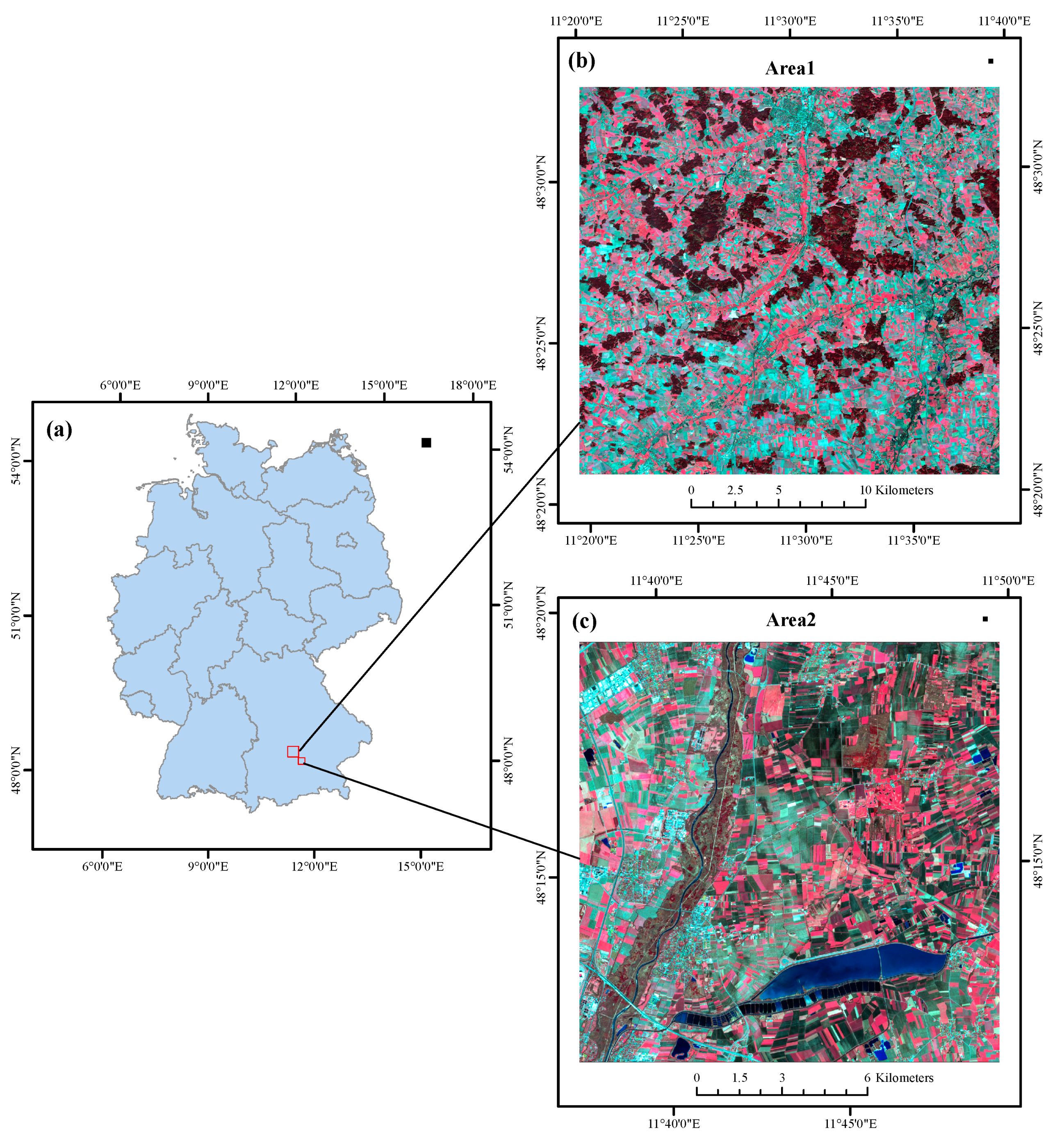
2. Study Area and Dataset

This study used the suburbs to the north of Munich, Germany, as the study area (Figure 1). The first experimental site (Study Area 1) is far from the urban area of Munich, covering an area of approximately 53,731 ha, which mainly includes (coniferous) forests, grasslands, maize fields, cereal fields, and artificial land. Thus, this area is sufficiently representative of agricultural areas. The second site (Study Area 2) is located closer to the actual urban extent of Munich and covers an area of ~21,726 ha. The primary land-cover types are (mixed and broad-leaved) forests, water bodies, maize fields, cereal fields, and artificial land. Study Area 2 can be used to examine the mapping of suburban areas.

The optical Sentinel images (Level-2A) were downloaded from the Copernicus Open Access Hub (https://scihub.copernicus.eu/dhus/#/home). We selected temporal images with <20% cloud coverage according to the metadata, acquired between January and December 2018, yielding a total of 39 images. Subsequently, Study Areas 1 and 2 were extracted by clipping. Cloud-free images for these areas were selected for subsequent classification analysis to explore how the time-series images impact the OBIA. Thus, stacks of 20 and 22 images were obtained for Study Areas 1 and 2, respectively (see

Table A1. Sentinel 2 image scenes and the corresponding date selected by sub-areas.

Selected by Area 1	Selected by Area 2	File Name of Sentinel 2 Image Scenes
2 April 2018	2 April 2018	S2A_MSIL2A_20180402T102021_N0207_R065_T32UPU_20180402T155007
7 April 2018	7 April 2018	S2B_MSIL2A_20180407T102019_N0207_R065_T32UPU_20180407T143030
19 April 2018	19 April 2018	S2A_MSIL2A_20180419T101031_N0207_R022_T32UPU_20180419T111252
22 April 2018	22 April 2018	S2A_MSIL2A_20180422T102031_N0207_R065_T32UPU_20180422T141352
27 April 2018	27 April 2018	S2B_MSIL2A_20180427T102019_N0207_R065_T32UPU_20180427T123359
7 May 2018	7 May 2018	S2B_MSIL2A_20180507T102019_N0207_R065_T32UPU_20180507T125310
1 July 2018	1 July 2018	S2A_MSIL2A_20180701T102021_N0208_R065_T32UPU_20180701T141038
31 July 2018	31 July 2018	S2A_MSIL2A_20180731T102021_N0208_R065_T32UPU_20180731T133841
2 August 2018	2 August 2018	S2B_MSIL2A_20180802T101019_N0208_R022_T32UPU_20180926T110335
12 August 2018	12 August 2018	S2B_MSIL2A_20180812T101019_N0208_R022_T32UPU_20180812T153601
17 August 2018	17 August 2018	S2A_MSIL2A_20180817T101021_N0208_R022_T32UPU_20180817T150139
20 August 2018	-	S2A_MSIL2A_20180820T102021_N0208_R065_T32UPU_20180820T161429
22 August 2018	22 August 2018	S2B_MSIL2A_20180822T101019_N0208_R022_T32UPU_20180822T161243
-	27 August 2018	S2A_MSIL2A_20180827T101021_N0208_R022_T32UPU_20180827T152355
16 September 2018	16 September 2018	S2A_MSIL2A_20180916T101021_N0208_R022_T32UPU_20180916T132415
4 October 2018	-	S2B_MSIL2A_20181004T102019_N0208_R065_T32UPU_20181004T151558
11 October 2018	11 October 2018	S2B_MSIL2A_20181011T101019_N0209_R022_T32UPU_20181011T131546
14 October 2018	14 October 2018	S2B_MSIL2A_20181014T102019_N0209_R065_T32UPU_20181014T165307
16 October 2018	16 October 2018	S2A_MSIL2A_20181016T101021_N0209_R022_T32UPU_20181016T131706
-	21 October 2018	S2B_MSIL2A_20181021T101039_N0209_R022_T32UPU_20181021T151822
18 November 2018	18 November 2018	S2A_MSIL2A_20181118T102311_N0210_R065_T32UPU_20181118T120023
-	20 November 2018	S2B_MSIL2A_20181120T101319_N0210_R022_T32UPU_20181120T151547
-	18 December 2018	S2A_MSIL2A_20181218T102431_N0211_R065_T32UPU_20181218T115057
28 December 2018	28 December 2018	S2A_MSIL2A_20181228T102431_N0211_R065_T32UPU_20181228T114836

in Appendix A). Given that images with high spatial resolution are preferred in OBIA [19], only the 10 m resolution bands (R, G, B, and near-infrared (NIR)) of the optical Sentinel images were employed in this study.

3. Methods

Figure 2 presents the main steps employed to assess the uncertainty caused by integrating OBIA with SITS data. After preparing the data (e.g., clipping and stacking) as mentioned above, the input data that satisfied the conditions for both areas were generated. Then, a sampling process was conducted to generate the reference layer for labeling the segmented objects. Segmentation based on the multi-temporal images was then performed to delimit the outlines of homogeneous areas for classification. Feature selection, as an optional process, was carried out before RF classification. We note that it is possible to repeat the classification process by randomly separating the labeled objects to obtain enough classification accuracy records and serve various uncertainty analysis evaluations.

3.1. Segmentation of Multi-Temporal Images

Multi-resolution segmentation is used [29] to partition the images into homogeneous objects. This step is realized using the eCognition 9.0 commercial software. For segmentation, the red, green, blue, and near-infrared spectral bands for six images from Study Area 1 and seven images from Study Area 2 (Figure 3) were used because a large number of images yield complex segmentation. Images for an entire calendar year (corresponding to the solid triangles in Figure 3) were used for segmentation to account for the characteristics of crop phenology, resulting in stacks of 24 and 28 layers for Study Areas 1 and 2, respectively. Here, the general parameter setting suggestions for multi-resolution segmentation were followed to ensure that the spectral information had the most important role during segmentation [18]; the color/shape parameters were set to 0.9/0.1 and the smoothness/compactness ratio was set to 0.5/0.5. The size of the segmented objects was controlled by the scale parameter (homogeneity threshold). Subsequently, different segmented layers were generated from scale 40 to 150 at increments of 10 to analyze the impact of scales on the accuracy of multi-temporal object-based classification; this has rarely been addressed in previous studies. Then, the segmentation results with feature information for each scale were exported for classification using Visual Studio 2010 and ArcEngine 10.0.

3.2. Training and Validation of Data Collection

To obtain sample objects for classification, polygon-shaped sampling units were generated and labeled. For this step, visual interpretation keys were used based on expert knowledge and crop phenology information from the European Land Use and Coverage Area Frame Survey (LUCAS) and the CORINE Land-Cover (CLC) data updated in 2018. Subsequently, these reference polygons were obtained manually;

Table 1. Redefining classes combining CORINE Land-Cover (CLC) and European Land Use and Coverage Area Frame Survey (LUCAS), with the total sample area of each class for both study sites.

Defined Class	CLC Description	LUCAS Description	Study Area 1 (ha)	Study Area 2 (ha)
Maize—11	211-Non-irrigated arable land	B16-Maize	1.1728	501.3447
Rapeseed—12		B32-Rape and turnip rape	0.6796	-
Cereals—13		B11-Common wheat B13-Barley B15-Oats	1.1603	290.0912
Forest—2	312-Coniferous forest 313-Mixed forest311-Broadleaved forest	C21-Coniferous woodland C31, C32-Mixed woodland C10-Broadleaved woodland	17.2707	762.3008
Artificial land—3	111-Continuous urban fabric 112-Discontinuous urban fabric 121-Industrial or commercial units	A22-Artificial non-built up areas A11, A12-Roofed built-up areas	6.1375	738.8659
Grassland—4	231-Pastures	E20-Grassland without tree/shrub cover E10-Grassland with sparse tree/shrub cover	2.4517	236.0831
Water areas—5	512-Water bodies	G10-Inland water bodies	0.2653	726.3547

lists the total sample area of each class for both study sites. Then, the segmented objects at each segmentation scale were labeled according to the 50% overlap rule with these reference polygons [30]. Subsequently, 30% of the labeled objects were selected as training samples using the stratified random sampling strategy [18], whereas all of the labeled objects were used for validation.

When utilizing CLC and LUCAS data for interpretation to obtain a reference layer, if the definitions of the CLC classes differ from those of the LUCAS classes, the latter were adopted. However, as barley (class B13), common wheat (class B11), and oats (class B15) have similar growth cycles and there were limited samples of barley and oat classes in the LUCAS dataset for the experimental sites, they were all recognized as cereals in this study. Table 1 lists the detailed definition principles, which also provides the relationship between the classes defined in this study and those of the CLC and LUCAS systems.

3.3. Classification Using Random Forest

Since its proposal by Breiman [31], the RF classification algorithm has been proven to outperform other supervised algorithms in extracting information from remote-sensing images [32,33]. As its name suggests, the algorithm randomly constructs a forest consisting of many interdependent decision trees. After the forest is constructed using training samples, if new samples must be classified, all decision trees are employed to make separate decisions. These decisions are taken as votes and the sample is classified into the class with the highest number of votes. Based on previous studies [32], in this study, the RF model used 479 trees and one randomly split variable; the ‘randomForest’ R package was integrated into the Visual Studio platform to implement classification for all of the images from both study areas.

3.4. Filtering Feature Subset and Temporal Characteristics Analysis

To obtain feature patterns in a season, the frequency of features selected were evaluated for different periods. This differs from the approach of evaluating an individual feature using the feature importance index. Therefore, correlation-based feature selection (CFS) [34] was used to calculate the frequency of the selected features. The CFS assesses the worth of a set of features using a heuristic evaluation function based on the correlation of features, and has been proven to be suitable for object-based classification in our previous study [24].

For feature evaluation and classification, the 20 images from Study Area 1 and 22 images from Study Area 2 were used. In this experiment, the inputs of the features for feature evaluation were derived from the red, green, blue, and near-infrared spectral bands of 10-m-resolution Sentinel data, resulting in stacks of 80 and 88 features for Study Areas 1 and 2, respectively. CFS was applied to these features repeatedly, maintaining a constant segmentation scale. This enabled the identification of the most used features in a certain period to determine the feature pattern in multi-temporal object-based classification.

3.5. Accuracy Evaluation and Statistical Tests

In this study, multi-temporal object-based classification was evaluated in terms of the overall accuracy (OA) and user’s accuracy (UA) metrics. These metrics were calculated using the area-based accuracy evaluation framework [35]. The OA was used to analyze the uncertainty of the segmentation scale, the number of images used, and the feature pattern. UA was employed to analyze the class-specific classification uncertainty influenced by the number of images used and the image scale. In addition, Welch’s t-test was conducted to compare the results obtained with and without feature selection.

4. Results

4.1. Influence of Multi-Temporal Images and Segmentation Scale on Overall Accuracy (OA)

First, the relationship between the image number/segmentation scale and OA was assessed. This was completed by classifying the samples from both study areas at various scales and incrementally increasing the number of input images. For this purpose, new images were added consecutively based on their DOY attribute. The contours in Figure 4a,b show the change pattern of the OA with regard to the segmentation scale and number of images used for both areas. From Figure 4, the influence of the number of images used on classification accuracy is much stronger than that of the segmentation scale, such that the accuracy increases steadily with the number of images used (Figure 4a,b). When the maximum number, i.e., 20, of images are used, up to 80 features are utilized. However, the RF classifier can still effectively use the multi-temporal spectral information and the results do not exhibit a significant Hughes phenomenon (Hughes phenomenon states that excessive features may lead to a negative impact on the classification accuracy) [36]. This may be attributed to the fact that images can contribute to the classification performance regardless of their specific acquisition time because of the different growth stages of crops [37]. We note that the results of this study are not consistent with those presented by Stromann et al. [28] because they argue that dimensionality reduction should be a key step in land-cover classification using SVM; however, this discrepancy can be attributed to the usage of the sensitive SVM.

To analyze the classification stability with changes in the segmentation scale, the mean value and mean square error of the classification accuracies of different segmentation scales (from scale 40 to 150, with an increment of 10) were calculated with a changing number of images. Figure 5 shows the results in the form of error bars, which indicates that the classification results at different scales differ more significantly when fewer images are included. In contrast, when more images are used during classification, scale variations have less of an influence on the classification accuracy (see Figure 5). Hence, we suggest that the use of multi-temporal data significantly alleviates the problem of identifying the “optimal” segmentation scale. This result is important because it means that selection of scales is less important in OB-SITS mapping, which until now, has been a particularly difficult task in OBIA [18,19]. Furthermore, owing to this novel finding, the integration of OBIA and time-series analysis becomes more feasible.

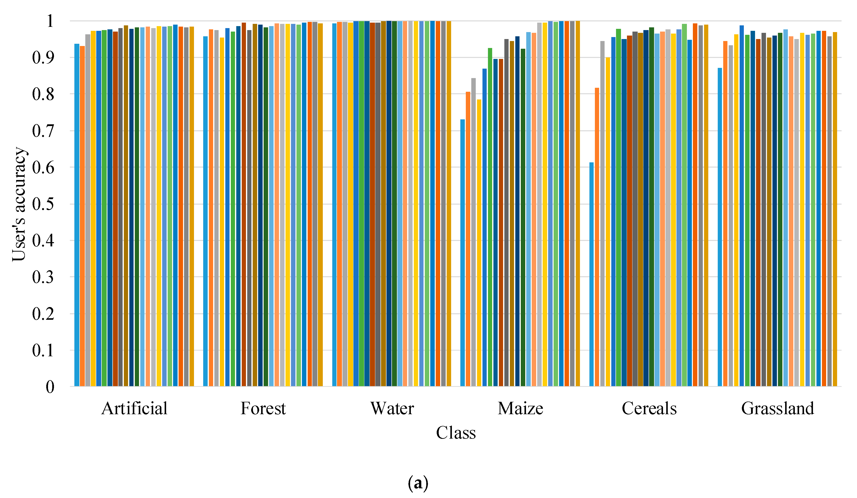
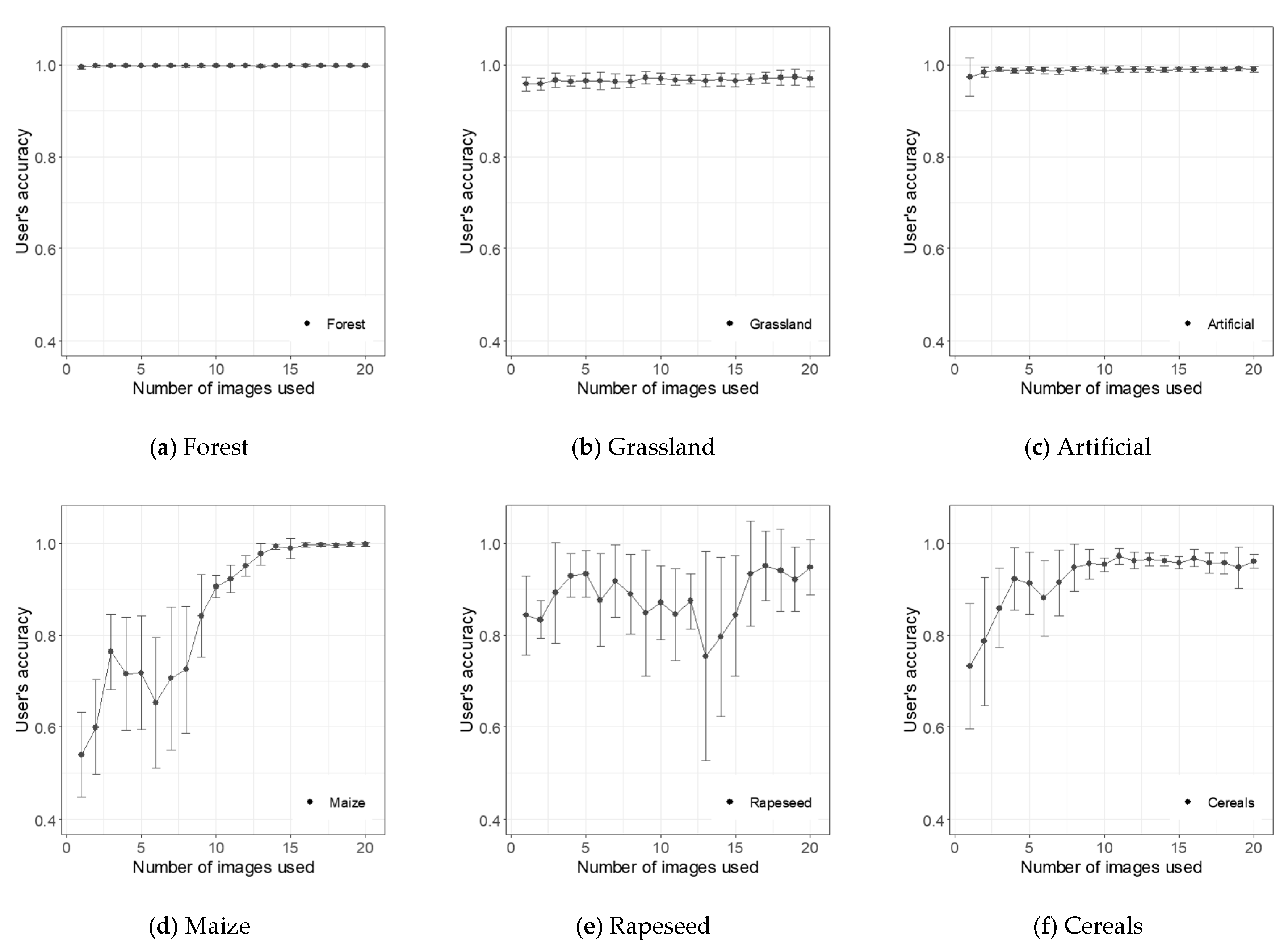
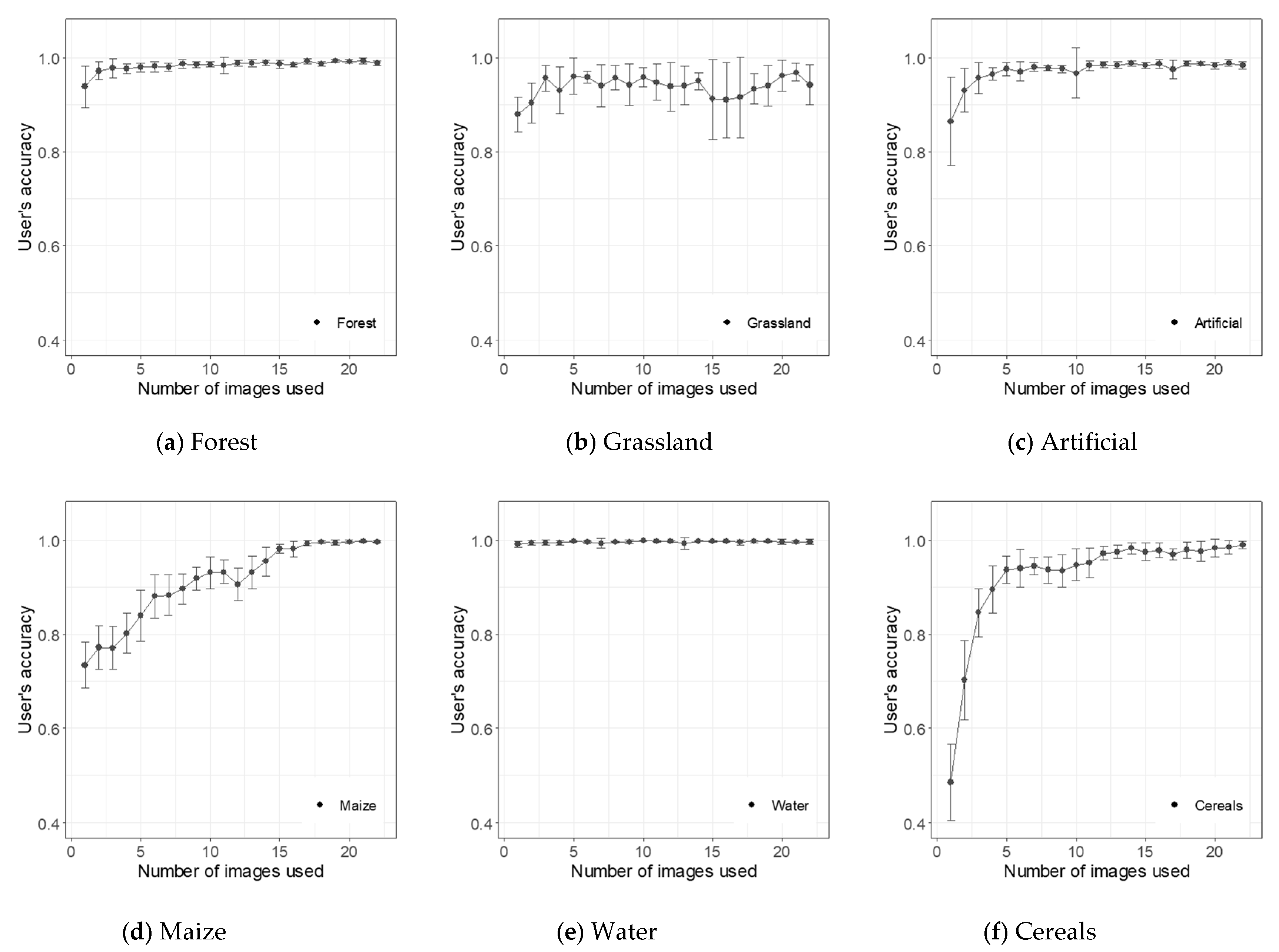
4.2. Effect of Multi-Temporal Images on Category Accuracy

Here, the UA index was used to evaluate the class-specific classification uncertainty. According to the previous analysis of the OA, the segmentation scales have less influence on accuracy than the number of images used. Therefore, this section examines the effects of the number of images used on the classification accuracy for different classes. For this purpose, bar charts were plotted to show the classification accuracy for different classes with different numbers of images. The results show that the accuracies of seasonal crops (maize, cereals, and rapeseed) generally increased when using an increasing number of input images (see Figure 6 and Figure 7).

Figure 6 and Figure 7 also show that the classification quality for winter or summer crops is significantly affected by the time of data retrieval. For both areas, we observed that the potential to classify summer crops (maize) increased from spring to summer and stabilized toward late summer to autumn. For both winter crops (rapeseed and cereals), the input of winter images was necessary to improve the performance, especially in the case of rapeseed. The rapeseed classification performance decreased with the input of summer images; this effect was most notable when the segmentation scale was large. However, the use of all images in the same year improved the classification performance of rapeseed (see Figure 6). In contrast, the classification accuracy for forests, grasslands, and artificial lands remained almost unchanged even if more images were used. This can be attributed to their spectral information being relatively stable throughout the year because the forest area in Study Area 1 is almost completely covered by coniferous forest. Despite this, we observed improvements in the accuracy for artificial lands and forests in Study Area 2 when more images were included as input (Figure 7). This is likely because this study area is closer to the urban area of Munich. Urban areas in Study Area 2 are more complicated due to the presence of various types of vegetation; a significant proportion of the forest areas in Study Area 2 comprise mixed and broad-leaved forests. This is the reason why Mendili et al. [38] adopted optical Sentinel time-series data in urban mapping; they suggested that the vegetation in an urban area affects the mapping of that area.

Based on the above analysis, we can conclude that the effect of the time of data retrieval on the classification quality can be explained with respect to the development stages of winter and summer crops. Furthermore, the recommendations for feature selection in the frame of crop mapping proposed by Veloso et al. [37] are acceptable. However, a decreasing trend was not observed in the classification accuracy for a single class when all images were used as input. Instead, a notable increase was observed in the classification accuracy of seasonal crops. Therefore, we recommend the use of as many Sentinel-2 images as possible within the year of interest to ensure an optimal classification performance, especially when the optical data in the time-series are not numerous (approximately 20 timestamps). Furthermore, excluding images from certain periods is not advised.

4.3. Effect of Segmentation Scale on Category Accuracy

To analyze the change pattern of the classification of a specific class, error bars with the mean value and mean square error were plotted to show the change in the UA for different classes when the number of images used was different (Figure 8 and Figure 9). As mentioned in the previous section, Figure 8 and Figure 9 show that the accuracies of seasonal crops (e.g., maize and cereals) benefit more from an increasing number of input images. More importantly, as revealed by the error bars, when more images are used, there is a reduction in the fluctuation of the accuracy of seasonal crops caused by segmentation scale variations (Figure 8 and Figure 9). This phenomenon was observed in the overall classification accuracy (Figure 5).

The findings of this study are slightly different from those reported by Löw et al. [8]. According to Löw et al. [8], constantly accurate classification can be achieved using, in general, five images. They stated that dense Sentinel or Landsat data exhibit no advantages in time-series classification. However, this study demonstrates that using more images enhances the classification accuracy due to the contribution of additional images to seasonal crop recognition. Thus, we recommend that image selection should not be applied in multi-temporal object-based classification.

4.4. Feature Selection Response

The classification was repeated 10 times with CFS for each segmentation scale and the frequency of the feature selected was calculated. In this section, for conciseness, only the experimental results for Study Area 1 are shown. In Figure 10, the size of the dot indicates the selected frequency of a specific band (y-axis) and date (x-axis) in the classification models. Only the 10 m resolution bands were evaluated. When only the acquisition time is considered, images taken in all seasons can be used with an equal frequency, except for images taken during the spring–summer transition in June. In contrast, based on comparisons of the frequencies at which different bands are selected, for the winter season, we observe that bands 3 and 4 are often not chosen in winter while bands 1 and 2 contribute more. This is likely because different bands respond to crops differently. For example, band 4 (NIR) is relatively sensitive to vegetation. However, vegetation coverage is less in winter; hence, the NIR band cannot contribute significantly to analyses during this period. In summary, Sentinel images acquired over all four seasons yield significant contributions to the classification of agricultural areas. Hence, images taken during a certain period of time must not be excluded without careful inspection and consideration. Moreover, we do not recommend filtering imported data based on a timeline, which has been conducted in most previous object-based multi-temporal classification studies (e.g., Vieira et al. [39]).

In addition, the classification was repeated 10 times for each scale with or without feature selection, followed by Welch’s t-test to compare their performance. From

Table 2. Differences between classification accuracies with or without feature selection based on Welch’s t-test.

Scale	50	60	70	80	90	100	110	120	130	140	150
p value	0.012	0.393	0.449	0.158	0.870	0.263	0.454	0.211	0.672	0.175	0.679

, all of the p-values are more than the significance level of alpha = 0.05, except at scale 50. Therefore, for almost all segmentation scales, we can conclude that the mean value of the classification accuracies with feature selection is not significantly different from that with all features. Hence, according to the experimental results, feature selection is not required when RF classifiers are used. This is possible because RF classifiers themselves can overcome the limitations of dimensionality more satisfactorily than other classifiers [20].

5. Conclusions

In this study, object-based land-cover classification using RF was applied to time-series optical Sentinel data. A systematic evaluation was conducted to understand classification uncertainty in object-based dense multi-temporal image classification, including the impact of the segmentation scale, spectral features, categories, frequency, and acquisition timing of optical satellite images. Subsequently, several important findings were obtained regarding the input of time-series data and the optimization of the segmentation scale.

The use of multi-temporal data significantly alleviates the problem associated with identifying an “optimal” segmentation scale. This finding is important because this makes the selection of scales, which was a challenge in OBIA, less important in OB-SITS mapping. As a result, the integration of OBIA and time-series analysis becomes more feasible. The findings of this study provide a scientific basis for the future application of Sentinel time-series data in conventional object-based supervised land-cover classification. We recommend the use of as many images as possible to enhance classification performance. Feature selection is an optional process when only limited Sentinel 2 images (e.g., approximately 20 timestamps) are used with RF as the classifier.

References

1. Zhu, Z.; Wulder, M.A.; Roy, D.P.; Woodcock, C.E.; Hansen, M.C.; Radeloff, V.C.; Healey, S.P.; Schaaf, C.; Hostert, P.; Scambos, T.A.; et al. Benefits of the free and open Landsat data policy. Remote Sens. Environ. 2019, 224, 382–385. [Google Scholar] [CrossRef]
2. Tatsumi, K.; Yamashiki, Y.; Torres, M.A.C.; Taipe, C.L.R. Crop classification of upland fields using Random forest of time-series Landsat 7 ETM+ data. Comput. Electron. Agric. 2015, 115, 171–179. [Google Scholar] [CrossRef]
3. Gómez, C.; White, J.C.; Wulder, M.A. Optical remotely sensed time series data for land cover classification: A review. ISPRS J. Photogramm. Remote Sens. 2016, 116, 55–72. [Google Scholar] [CrossRef] [Green Version]
4. Pelletier, C.; Valero, S.; Inglada, J.; Champion, N.; Dedieu, G. Assessing the robustness of Random Forests to map land cover with high resolution satellite image time series over large areas. Remote Sens. Environ. 2016, 187, 156–168. [Google Scholar] [CrossRef]
5. Vuolo, F.; Neuwirth, M.; Immitzer, M.; Atzberger, C.; Ng, W.T. How much does multi-temporal Sentinel-2 data improve crop type classification? Int. J. Appl. Earth Obs. Geoinf. 2018, 72, 122–130. [Google Scholar] [CrossRef]
6. Zhang, X.; Liu, L.; Chen, X.; Xie, S.; Gao, Y. Fine land-cover mapping in China using Landsat datacube and an operational SPECLib-Based approach. Remote Sens. 2019, 11, 1056. [Google Scholar] [CrossRef] [Green Version]
7. Zhang, M.; Lin, H. Object-based rice mapping using time-series and phenological data. Adv. Space Res. 2019, 63, 190–202. [Google Scholar] [CrossRef]
8. Löw, F.; Knöfel, P.; Conrad, C. Analysis of uncertainty in multi-temporal object-based classification. ISPRS J. Photogramm. Remote Sens. 2015, 105, 91–106. [Google Scholar] [CrossRef]
9. Zhu, Z.; Gallant, A.L.; Woodcock, C.E.; Pengra, B.; Olofsson, P.; Loveland, T.R.; Jin, S.; Dahal, D.; Yang, L.; Auch, R.F. Optimizing selection of training and auxiliary data for operational land cover classification for the LCMAP initiative. ISPRS J. Photogramm. Remote Sens. 2016, 122, 206–221. [Google Scholar] [CrossRef] [Green Version]
10. Cai, Y.; Li, X.; Zhang, M.; Lin, H. Mapping wetland using the object-based stacked generalization method based on multi-temporal optical and SAR data. Int. J. Appl. Earth Obs. Geoinf. 2020, 92, 102164. [Google Scholar] [CrossRef]
11. Ienco, D.; Gaetano, R.; Interdonato, R.; Ose, K.; Minh, D.H.T. Combining Sentinel-1 and Sentinel-2 Time Series via RNN for object-based land cover classification. In Proceedings of the IEEE International Geoscience and Remote Sensing Symposium, Yokohama, Japan, 28 July–2 August 2019. [Google Scholar]
12. Belgiu, M.; Csillik, O. Sentinel-2 cropland mapping using pixel-based and object-based time-weighted dynamic time warping analysis. Remote Sens. Environ. 2017, 204, 509–523. [Google Scholar] [CrossRef]
13. Csillik, O.; Belgiu, M.; Asner, G.P.; Kelly, M. Object-based time-constrained dynamic time warping classification of crops using Sentinel-2. Remote Sens. 2019, 11, 1257. [Google Scholar] [CrossRef] [Green Version]
14. Maus, V.; Câmara, G.; Appel, M.; Pebesma, E. dtwSat: Time-weighted dynamic time warping for satellite image time series analysis in R. J. Stat. Softw. 2019, 88, 1–31. [Google Scholar] [CrossRef] [Green Version]
15. Pelletier, C.; Webb, G.I.; Petitjean, F. Temporal Convolutional Neural Network for the Classification of Satellite Image Time Series. Remote Sens. 2019, 11, 523. [Google Scholar] [CrossRef] [Green Version]
16. Luciano, A.C.D.S.; Picoli, M.C.A.; Rocha, J.V.; Duft, D.G.; Lamparelli, R.A.C.; Leal, M.R.L.V.; Maire, G.L. A generalized space-time OBIA classification scheme to map sugarcane areas at regional scale, using Landsat images time-series and the random forest algorithm. Int. J. Appl. Earth Obs. Geoinf. 2019, 80, 127–136. [Google Scholar] [CrossRef]
17. Brinkhoff, J.; Vardanega, J.; Robson, A.J. Land cover classification of nine perennial crops using sentinel-1 and -2 data. Remote Sens. 2020, 12, 96. [Google Scholar] [CrossRef] [Green Version]
18. Ma, L.; Cheng, L.; Li, M.; Liu, Y.; Ma, X. Training set size, scale, and features in Geographic Object-Based Image Analysis of very high resolution unmanned aerial vehicle imagery. ISPRS J. Photogramm. Remote Sens. 2015, 102, 14–27. [Google Scholar] [CrossRef]
19. Ma, L.; Li, M.; Ma, X.; Cheng, L.; Du, P.; Liu, Y. A review of supervised object-based land-cover image classification. ISPRS J. Photogramm. Remote Sens. 2017, 130, 277–293. [Google Scholar] [CrossRef]
20. Li, M.; Ma, L.; Blaschke, T.; Cheng, L.; Tiede, D. A systematic comparison of different object-based classification techniques using high spatial resolution imagery in agricultural environments. Int. J. Appl. Earth Obs. Geoinf. 2016, 49, 87–98. [Google Scholar] [CrossRef]
21. Rougier, S.; Puissant, A.; Stumpf, A.; Lachiche, N. Comparison of sampling strategies for object-based classification of urban vegetation from Very High Resolution satellite images. Int. J. Appl. Earth Obs. Geoinf. 2016, 51, 60–73. [Google Scholar] [CrossRef]
22. Ye, S.; Pontius, R.G.; Rakshit, R. A review of accuracy assessment for object-based image analysis: From per-pixel to per-polygon approaches. ISPRS J. Photogramm. Remote Sens. 2018, 141, 137–147. [Google Scholar] [CrossRef]
23. Laliberte, A.S.; Browning, D.M.; Rango, A. A comparison of three feature selection methods for object-based classification of sub-decimeter resolution UltraCam-L imagery. Int. J. Appl. Earth Obs. Geoinf. 2012, 15, 70–78. [Google Scholar] [CrossRef]
24. Ma, L.; Fu, T.; Blaschke, T.; Li, M.; Tiede, D.; Zhou, Z.; Ma, X.; Chen, D. Evaluation of feature selection methods for object-based land cover mapping of unmanned aerial vehicle imagery using random forest and support vector machine classifiers. ISPRS Int. J. Geo-Inf. 2017, 6, 51. [Google Scholar] [CrossRef]
25. Shirvani, Z.; Abdi, O.; Buchroithner, M.F. A synergetic analysis of Sentinel-1 and -2 for mapping historical landslides using object-oriented Random Forest in the Hyrcanian forests. Remote Sens. 2019, 11, 2300. [Google Scholar] [CrossRef] [Green Version]
26. Liu, B.; Du, S.; Du, S.; Zhang, X. Incorporating deep features into GEOBIA paradigm for remote sensing imagery classification: A patch-based approach. Remote Sens. 2020, 12, 3007. [Google Scholar] [CrossRef]
27. Abdi, O. Climate-triggered insect defoliators and forest fires using multitemporal Landsat and TerraClimate data in NE Iran: An application of GEOBIA TreeNet and panel data analysis. Sensors 2019, 19, 3965. [Google Scholar] [CrossRef] [Green Version]
28. Stromann, O.; Nascetti, A.; Yousif, O.; Ban, Y. Dimensionality reduction and feature selection for object-based land cover classification based on sentinel-1 and sentinel-2 time series using google earth engine. Remote Sens. 2020, 12, 76. [Google Scholar] [CrossRef] [Green Version]
29. Baatz, M.; Schäpe, A. Multiresolution Segmentation-an optimization approach for high quality multi-scale image segmentation. In Angewandte Geographische Informationsverarbeitung; Strobl, J., Blaschke, T., Griesebner, G., Eds.; Wichmann-Verlag: Heidelberg, Germany, 2000; pp. 12–23. [Google Scholar]
30. Radoux, J.; Bogaert, P. Accounting for the area of polygon sampling units for the prediction of primary accuracy assessment indices. Remote Sens. Environ. 2014, 142, 9–19. [Google Scholar] [CrossRef]
31. Breiman, L. Random Forests. Mach. Learn. 2001, 45, 5–32. [Google Scholar] [CrossRef] [Green Version]
32. Rodriguez-Galiano, V.F.; Ghimire, B.; Rogan, J.; Chica-Olmo, M.; Rigol-Sanchez, J.P. An assessment of the effectiveness of a random forest classifier for land-cover classification. ISPRS J. Photogramm. Remote Sens. 2012, 67, 93–104. [Google Scholar] [CrossRef]
33. Puissant, A.; Rougier, S.; Stumpf, A.E. Object-oriented mapping of urban trees using Random Forest classifiers. Int. J. Appl. Earth Obs. Geoinf. 2014, 26, 235–245. [Google Scholar] [CrossRef]
34. Hall, M.A.; Holmes, G. Benchmarking attribute selection techniques for discrete class data mining. IEEE Trans. Knowl. Data Eng. 2003, 15, 1437–1447. [Google Scholar] [CrossRef] [Green Version]
35. Radoux, J.; Bogaert, P. Good Practices for Object-Based Accuracy Assessment. Remote Sens. 2017, 9, 646. [Google Scholar] [CrossRef] [Green Version]
36. Pal, M.; Foody, G.M. Feature selection for classification of hyperspectral data by SVM. IEEE Trans. Geosci. Remote Sens. 2010, 48, 2297–2307. [Google Scholar] [CrossRef] [Green Version]
37. Veloso, A.; Mermoz, S.; Bouvet, A.; Toan, T.L.; Planells, M.; Dejoux, J.F.; Ceschia, E. Understanding the temporal behavior of crops using Sentinel-1 and Sentinel-2-like data for agricultural applications. Remote Sens. Environ. 2017, 199, 415–426. [Google Scholar] [CrossRef]
38. Mendili, L.; Puissant, A.; Chougrad, M.; Sebari, I. Towards a Multi-Temporal Deep Learning Approach for Mapping Urban Fabric Using Sentinel 2 Images. Remote Sens. 2020, 12, 423. [Google Scholar] [CrossRef] [Green Version]
39. Vieira, M.A.; Formaggio, A.R.; Rennó, C.D.; Atzberger, C.; Aguiar, D.A.; Mello, M.P. Object Based Image Analysis and Data Mining applied to a remotely sensed Landsat time-series to map sugarcane over large areas. Remote Sens. Environ. 2012, 123, 553–562. [Google Scholar] [CrossRef]
Figure 1. Study area. (a) Map of Germany; (b) images of Study Area 1; and (c) images of Study Area 2.
Remotesensing 12 03798 g001
Figure 2. The object-based satellite image time-series (OB-SITS) workflow. (a) The optical Sentinel images are first processed to create stacked input data. Based on the input data, (b) the sampling units are then extracted and (c) multi resolution segmentation is used to generate the segmentation objects. (d) The labelled objects are determined by the sampling units. (f) A random forest classifier is employed to classify the un-labelled objects. (e) Before classification, feature selection is an optional step to filter out redundant features. (g) The metrics of the overall and user’s accuracy are used to analyze the classification uncertainty.
Remotesensing 12 03798 g002
Figure 3. Images used for segmentation (solid triangles) and classification (all) for Areas 1 (a) and 2 (b). DOY = day of year.
Remotesensing 12 03798 g003
Figure 4. Changes in the overall accuracy (OA) with respect to the segmentation scale and number of images used by random forest (RF) in (a) Area 1 and (b) Area 2. The x-axis represents the segmentation scale and the y-axis represents the images used.
Remotesensing 12 03798 g004
Figure 5. The mean value of the OAs with different segmentation scales for specific images in Area 1 (circles) and Area 2 (triangles). Error bars indicate the mean square error for a certain number of images used.
Remotesensing 12 03798 g005
Figure 6. The user’s accuracy (UA) of each class with an increasing number of images used at different segmentation scales for Study Area 1. (a) Scale 50, (b) scale 100, and (c) scale 150. The colored bars from left to right represent the number of images from 1 to 20.
Remotesensing 12 03798 g006aRemotesensing 12 03798 g006b
Figure 7. The user’s accuracy (UA) of each class with an increasing number of images used at different segmentation scales for Study Area 2. (a) Scale 50, (b) scale 100, and (c) scale 150. The colored bars from left to right represent the number of images from 1 to 22.
Remotesensing 12 03798 g007aRemotesensing 12 03798 g007b
Figure 8. For Study Area 1, the mean UA of classification (repeated at 12 segmentation scales, from scale 40 to 150) and error bars indicate the mean square errors of different segmentation scales. (af) show forest, grassland, artificial land, maize, rapeseed, and cereals, respectively.
Remotesensing 12 03798 g008
Figure 9. For Study Area 2, the mean UA of classifications (repeated at 12 segmentation scales, from scale 40 to 150) and error bars indicate the mean square errors of different segmentation scales. (af) show forest, grassland, artificial land, maize, water, and cereals, respectively.
Remotesensing 12 03798 g009
Figure 10. Selected frequency of a specific band and date. Band numbers 1, 2, 3, and 4 indicate red, green, blue, and near-infrared (NIR), respectively.
Remotesensing 12 03798 g010