A Slimmer Network with Polymorphic and Group Attention Modules for More Efficient Object Detection in Aerial Images

Abstract

Object detection is one of the core technologies in aerial image processing and analysis. Although existing aerial image object detection methods based on deep learning have made some progress, there are still some problems remained: (1) Most existing methods fail to simultaneously consider multi-scale and multi-shape object characteristics in aerial images, which may lead to some missing or false detections; (2) high precision detection generally requires a large and complex network structure, which usually makes it difficult to achieve the high detection efficiency and deploy the network on resource-constrained devices for practical applications. To solve these problems, we propose a slimmer network for more efficient object detection in aerial images. Firstly, we design a polymorphic module (PM) for simultaneously learning the multi-scale and multi-shape object features, so as to better detect the hugely different objects in aerial images. Then, we design a group attention module (GAM) for better utilizing the diversiform concatenation features in the network. By designing multiple detection headers with adaptive anchors and the above-mentioned two modules, we propose a one-stage network called PG-YOLO for realizing the higher detection accuracy. Based on the proposed network, we further propose a more efficient channel pruning method, which can slim the network parameters from 63.7 million (M) to 3.3M that decreases the parameter size by 94.8%, so it can significantly improve the detection efficiency for real-time detection. Finally, we execute the comparative experiments on three public aerial datasets, and the experimental results show that the proposed method outperforms the state-of-the-art methods.

1. Introduction

Object detection in aerial images is an important research direction in the field of computer vision [1], and its development has great significance in both the civilian and military fields. In the civilian field, aerial image object detection technology is widely used in the real-time update of urban spatial database, urban planning, disaster detection, etc. In the military field, this technology has become an important means of military reconnaissance and early warning in the modern army. Despite many advanced methods based on deep learning [2,3] have succeeded in the natural image object detection, the development of object detection in aerial images is relatively slow because of the complicated backgrounds, overlooking views, and variations in scale and shape of the objects [4,5].

To detect the special objects of the different scales, the multi-scale image pyramid [6] is usually adopted. However, this method requires many calculations and memories, hence many object detectors have avoided the multi-scale image pyramid representation. From this, some researchers built the multi-scale pyramids based on the internal structure of the convolutional neural network (CNN) [7] to detect multi-scale targets, which only request a small number of additional computational cost. Some typical methods based on this idea are as follows. The feature pyramid network (FPN) [8] adopts a top-down structure and lateral connections for fusing the shallow layer features with low-level semantic information and the deep layer features with high-level semantic information, which enriches the features of the different scales. The single-shot multibox detector (SSD) [9] fuses the different scale features from the different layers to obtain the multi-scale features without additional calculation. The scale-aware trident network (TridentNet) [10] can generate the specific feature maps with different scales through a parallel multi-branch framework for which each branch owns the different receptive fields. YOLOv3 (You only look once) [3] is inspired by the FPN structure and introduces a similar feature pyramid structure to detect the objects with multi-scale. Although these advanced methods can improve the general multi-scale object detection effect to a certain extent, they are still unable to completely solve the huge differences in object scales and that in object shapes under complex background, thus cannot achieve the optimal effect in aerial image object detection. Generally speaking, aerial images are generally acquired from vertical vision with the different equipment and distance, variational weather and lighting conditions, so the background of the aerial image is generally very complex, and there are targets with vast differences in scale and that in shape. There are also some scholars who have proposed corresponding solutions for many objects with different shapes in aerial images. Qiu et al. [11] leveraged an aspect ratio attention network to select the region of interest (RoI) features that match the shapes of objects. Based on this, many objects with large aspect ratio differences in aerial images can also be referred to as multi-shape objects in object detection. In addition to Reference [11], Xu et al. [12] developed an aspect ratio constrained non-maximum suppression (arcNMS), and Yan et al. [13] proposed the class aspect ratio constrained non-maximum suppression (CARC-NMS) to remove the line like false region proposals (LFRP) during non-maximum suppression (NMS) process. But these two methods afore-mentioned are only suitable for removing the false detect results with abnormal aspect ratio caused by deformable convolution [14] in the network. 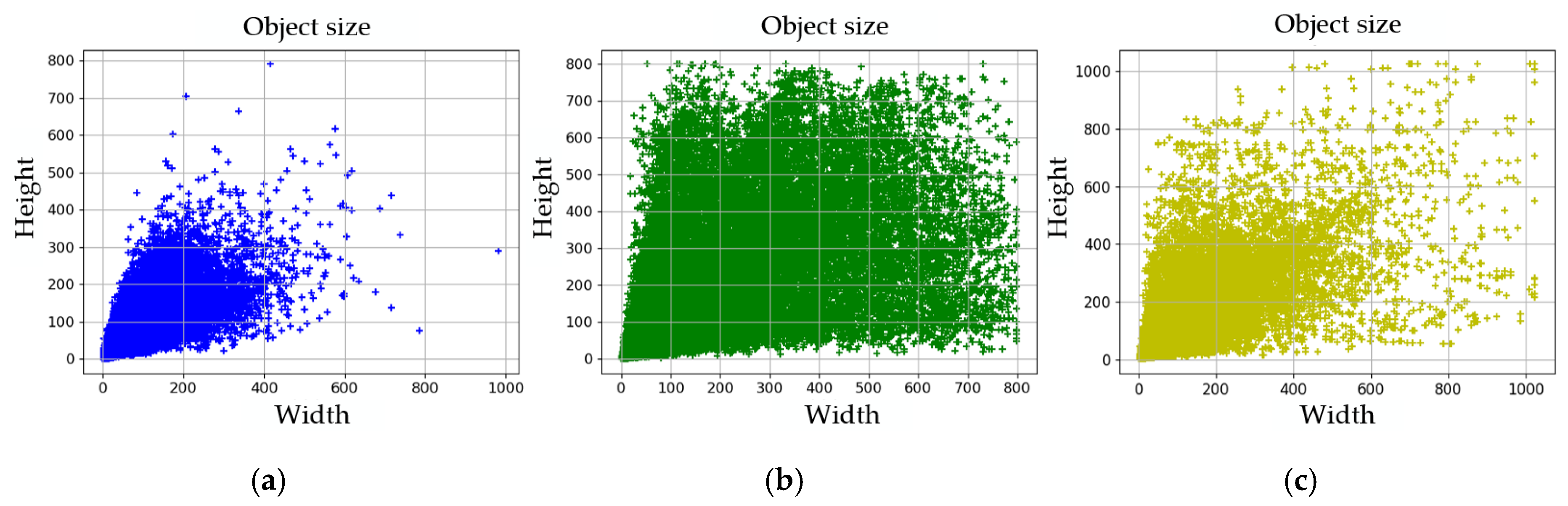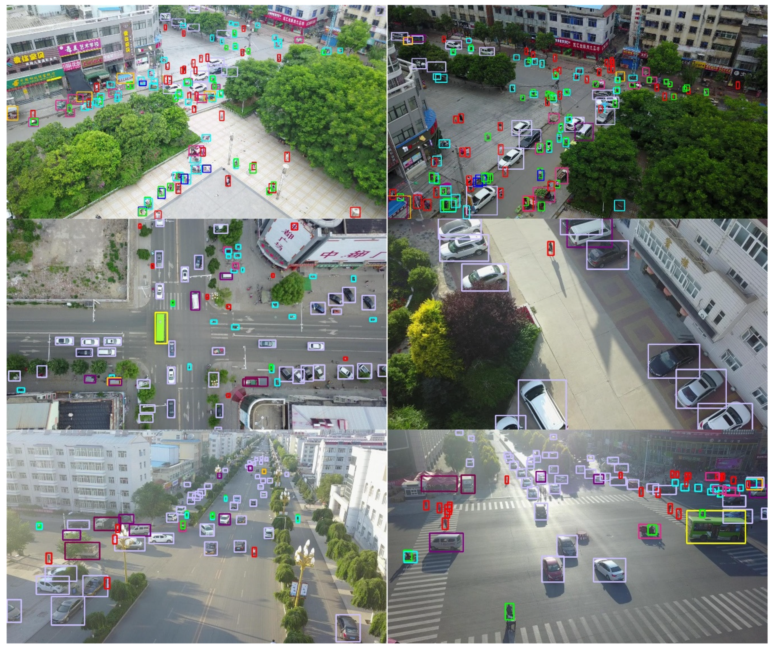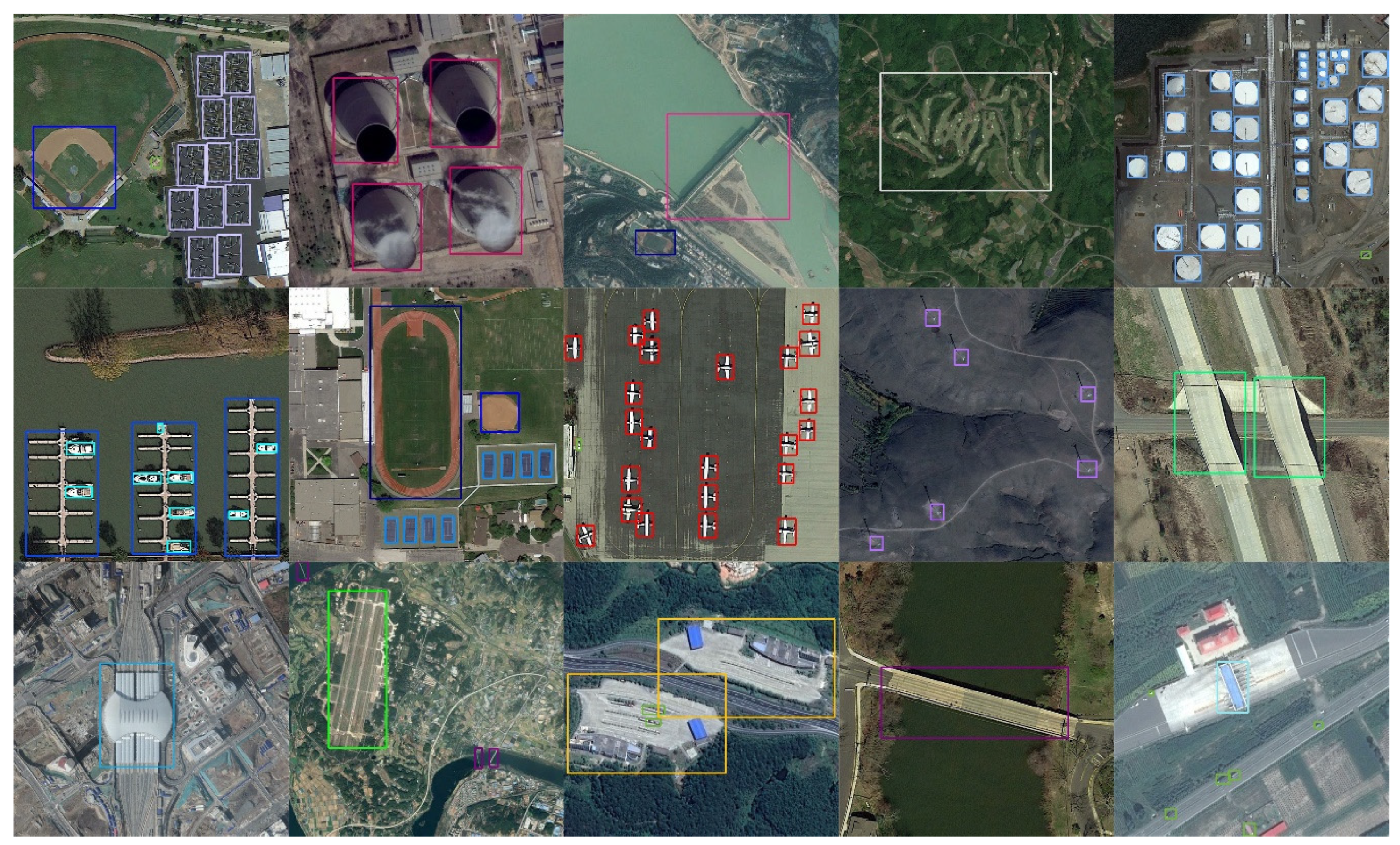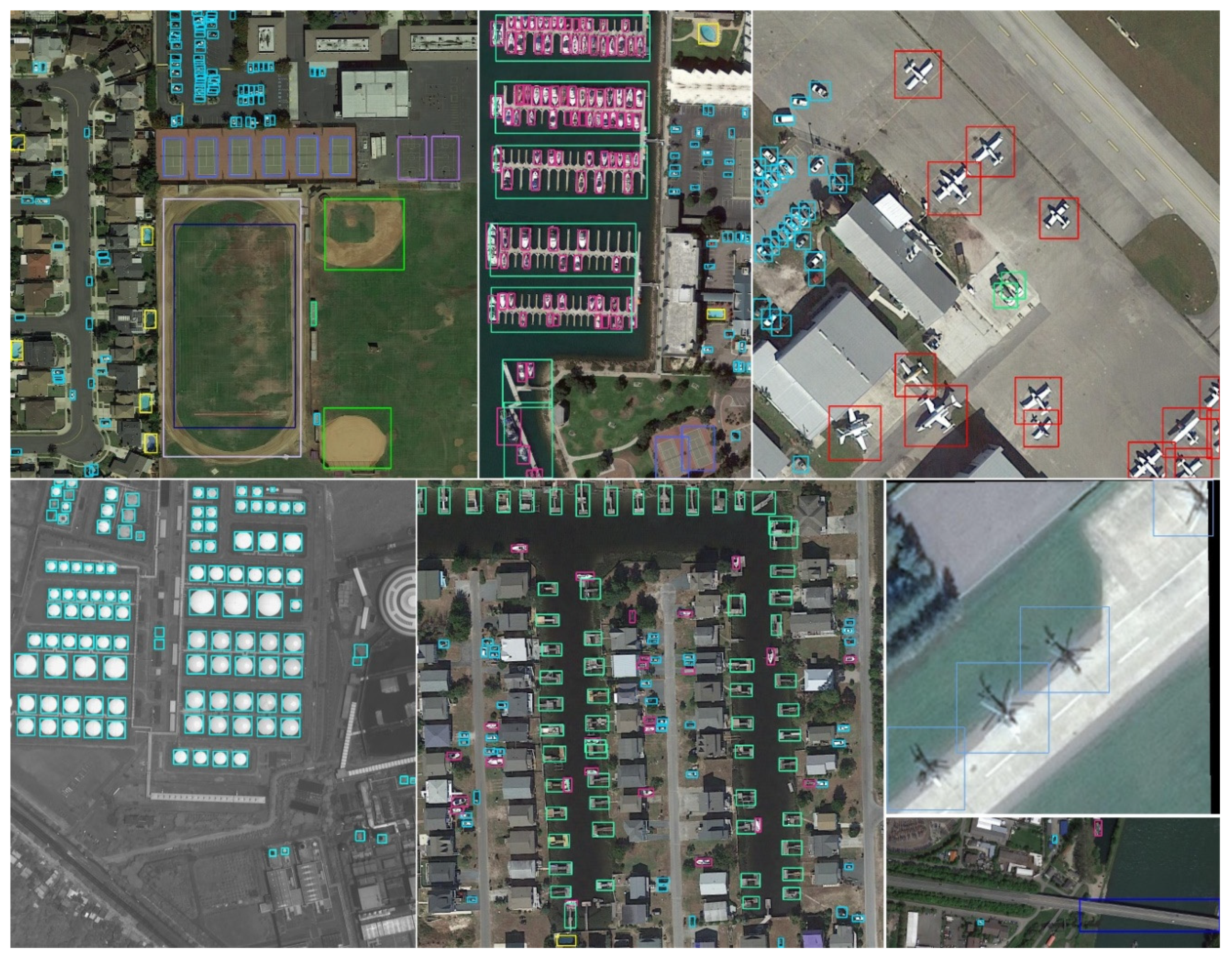Figure 1 displays some concrete examples of aerial images. From Figure 1, the scale of the bus in Figure 1c is much larger than that in Figure 1a. Moreover, the scales of the ships in Figure 1b,d are much smaller than the scales of the bridges and harbors. Moreover, the shapes of the bridges and harbors are also quite different from that of ordinary objects. It can be clearly seen from Figure 1b,d that the aspect ratios of the bridges and harbors are relatively large.

To solve the multi-scale object detection problems further better, in addition to the complex multi-scale network structures mentioned above, there are some well-designed modules that are embedded into the network to fuse the multi-scale features and can effectively detect the multi-scale objects. Figure 2 shows the details of four typical multi-scale fusion modules. The inception-v2 module [15] (a) uses the different convolutional kernels to extract multi-scale feature information. The spatial pyramid pooling (SPP) module [16] (Figure 2b) utilizes the pooling layers of the different sizes for fusing the multi-scale features. The atrous spatial pyramid pooling (ASPP) module [17] (Figure 2c) exploits multiple parallel atrous convolutional layers with different rates for extracting multi-scale feature information. Furthermore, the receptive field block (RFB) [18] (Figure 2d) uses multi-scale atrous convolutional layers to adapt to the different scale kernels of CNN, which can cover the different scale receptive fields and is very useful for obtaining multi-scale features. With reasonable design, these modules can effectively increase the multi-scale feature extraction capability of neural networks and further improve the effect of multi-scale object detection. However, the objects in aerial images generally not only differ in the scale, but also their shapes may also vary widely. As mentioned above, the aspect ratio of the bridge and harbor is very large, as shown in Figure 1b,d. Therefore, it is necessary to design more effective modules for realizing the more effective detection of the multi-scale and multi-shape targets in aerial images.

Moreover, when fusing the multi-scale or the multi-shape features, either by fusing the different scale features of different layers or by fusing the different scale or shape features of the different branches of the same layer, most of the existing methods [3,8] usually ignore the importance of each merged parts that are treated equally and through direct concatenation or addition on the channels with the uniform weights to merge the different features of the different layers or the different branches of the same layer. Therefore, this is not conducive to the neural network for making full use of the different features.

In addition, due to the complex background and the diversity of object scales and shapes in aerial images, a larger and more complex network model is usually required for obtaining more excellent detection accuracy. However, the larger network model is often large in volume, which will affect detection efficiency and make it difficult to deploy the network model on the resource-limited devices for real-time detection and practical applications. Besides, it is empirically known that larger network models generally contain many redundant information, thus some researchers [19,20,21,22,23,24] have proposed some model compression methods for reducing model volume and speeding up object detection. Among these model compression methods, the structural pruning [19,20,21,22,23], especially channel pruning [19,21,23], is widely used to reduce the number of model parameters and computing complexity. Nevertheless, the existing methods usually design a predefined global threshold [19,21] for all layers or the independent local threshold for each layer [23] to pruning unimportant channels for saving memory and decreasing inference time. It is worth noting that the absolute value of the scale factors in batch normalization (BN) [25] layers are generally used to measure the importance of each channel in the model, and the channel pruning threshold is also designed according to the scale factors [19,21,23]. But when designing the channel pruning threshold, the above-mentioned methods either only consider the value distribution of the global scale factors or only consider the value distribution of the local scale factors in the corresponding layers, so they cannot reach both the global optimality of all layers and the local optimality of each layer at the same time, and their performances are usually not optimal. Therefore, it is an urgent problem that how to propose a more suitable channel pruning method with the superior pruning threshold for achieving more efficient model compression and improving the object detection speed of aerial images without affecting the model accuracy.

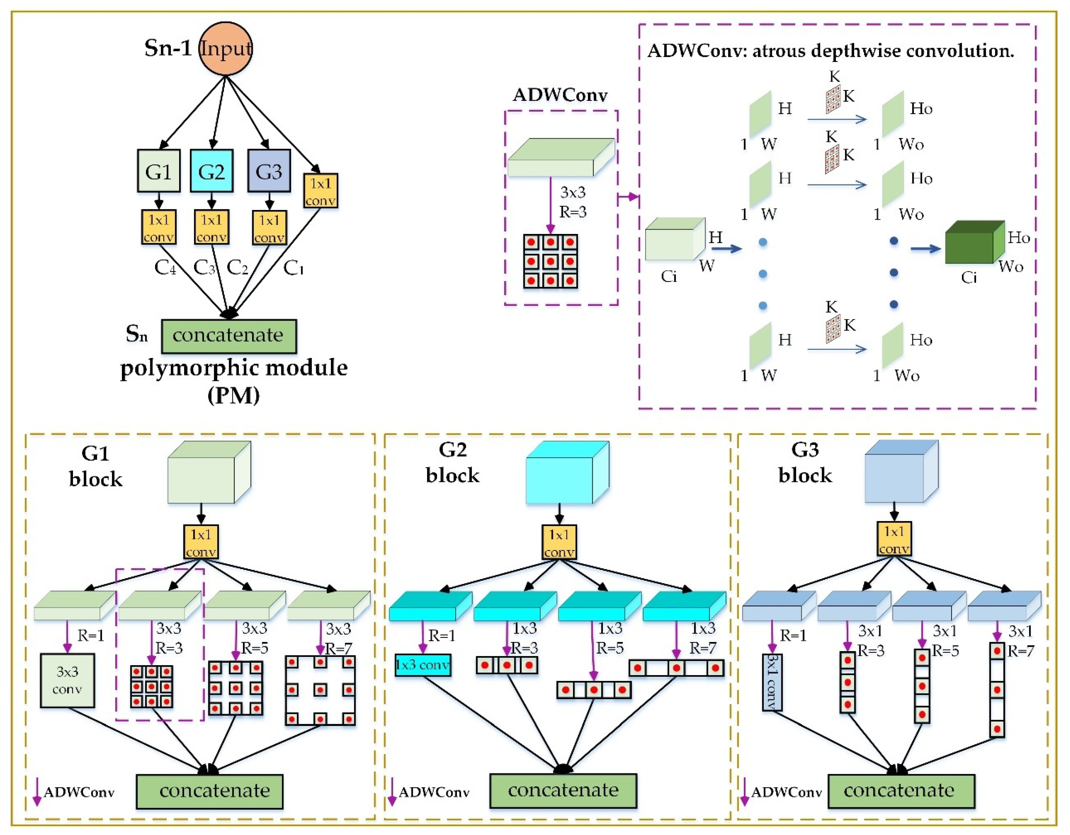
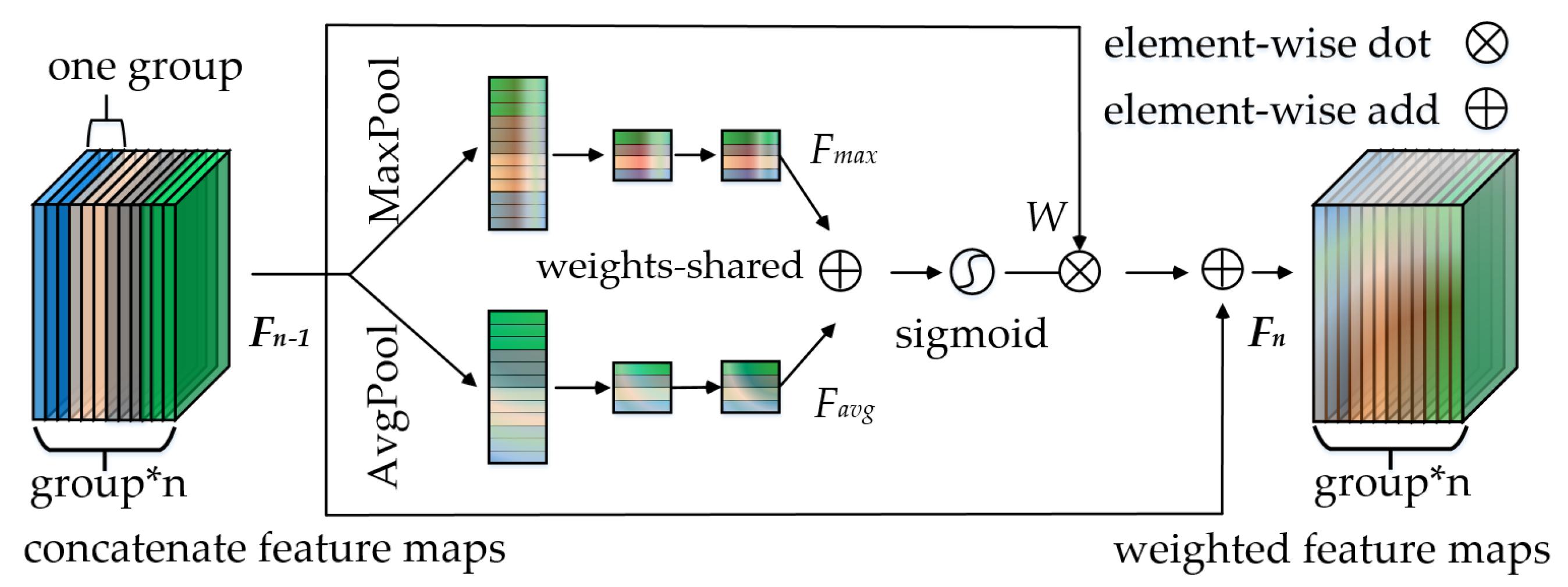
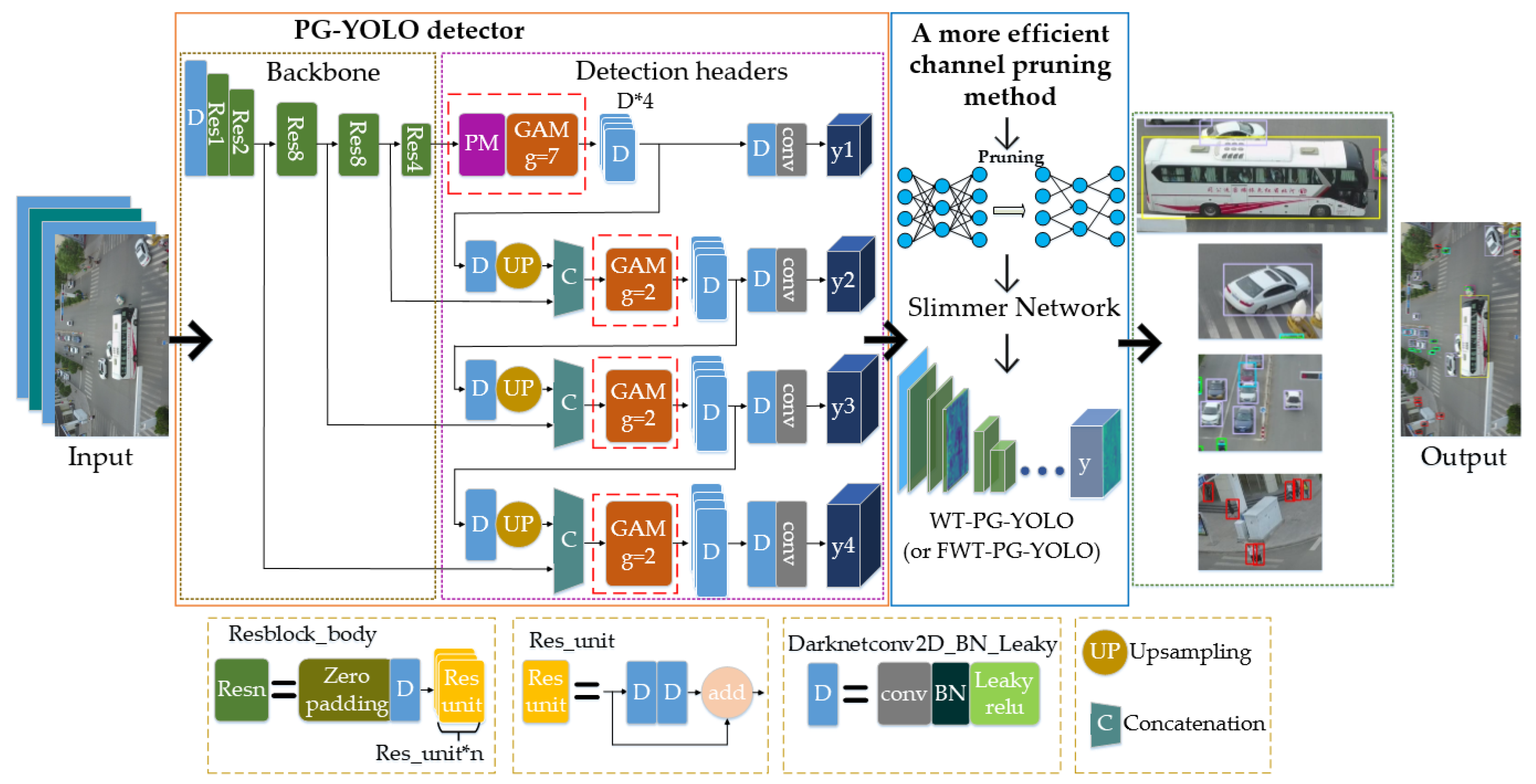
In this paper, to solve the above problems, we propose a slimmer network for more efficient object detection in aerial images. Firstly, we design a polymorphic module (PM) to simultaneously learn the characteristics of great differences in the object scales and that in the object shapes, so it can better detect the hugely different targets in aerial images. The well-designed PM can also enable the network to focus better on the key information of the objects from the background for achieving more accurate detection. Considering the concatenation of the different features using unified weights may not be able to utilize the feature information suitably and efficiently, we then design a group attention module (GAM) for better learning the different concatenate features in the network. Specifically, the GAM can assign different importance to the different concatenation layers. Based on the designed modules, we further propose a fast and accurate network called PG-YOLO (P, G represent the PM and GAM, respectively), which also employs multiple detection headers with adaptive anchors for the aerial image object detection. The baseline of this network is the currently excellent YOLOv3 [3]. Because we have devised a more reasonable and efficient network structure, the proposed PG-YOLO can achieve higher detection accuracy for multi-scale and multi-shape objects in aerial images. In addition, considering that the large network model tends to have a large model volume with some redundant information, which will affect detection efficiency and make it difficult to deploy the network model on the resource-limited devices for practical applications, we propose an efficient channel pruning method with a superior layer-wise weighted threshold to slim the network model and realize higher detection efficiency nearly without accuracy loss for real-time detection.

Our main contributions in this paper are as follows:

• We design a polymorphic module (PM) for learning the multi-scale and multi-shape object features simultaneously in aerial images. The PM is also able to make the network focus better on the key feature of the objects for achieving more accurate detection. Moreover, a group attention module (GAM) is designed for better utilizing the different concatenate features in the network.
• By devising multiple detection headers with adaptive anchors and the designed two modules, we propose a one-stage network called PG-YOLO for realizing the higher detection accuracy in aerial images.
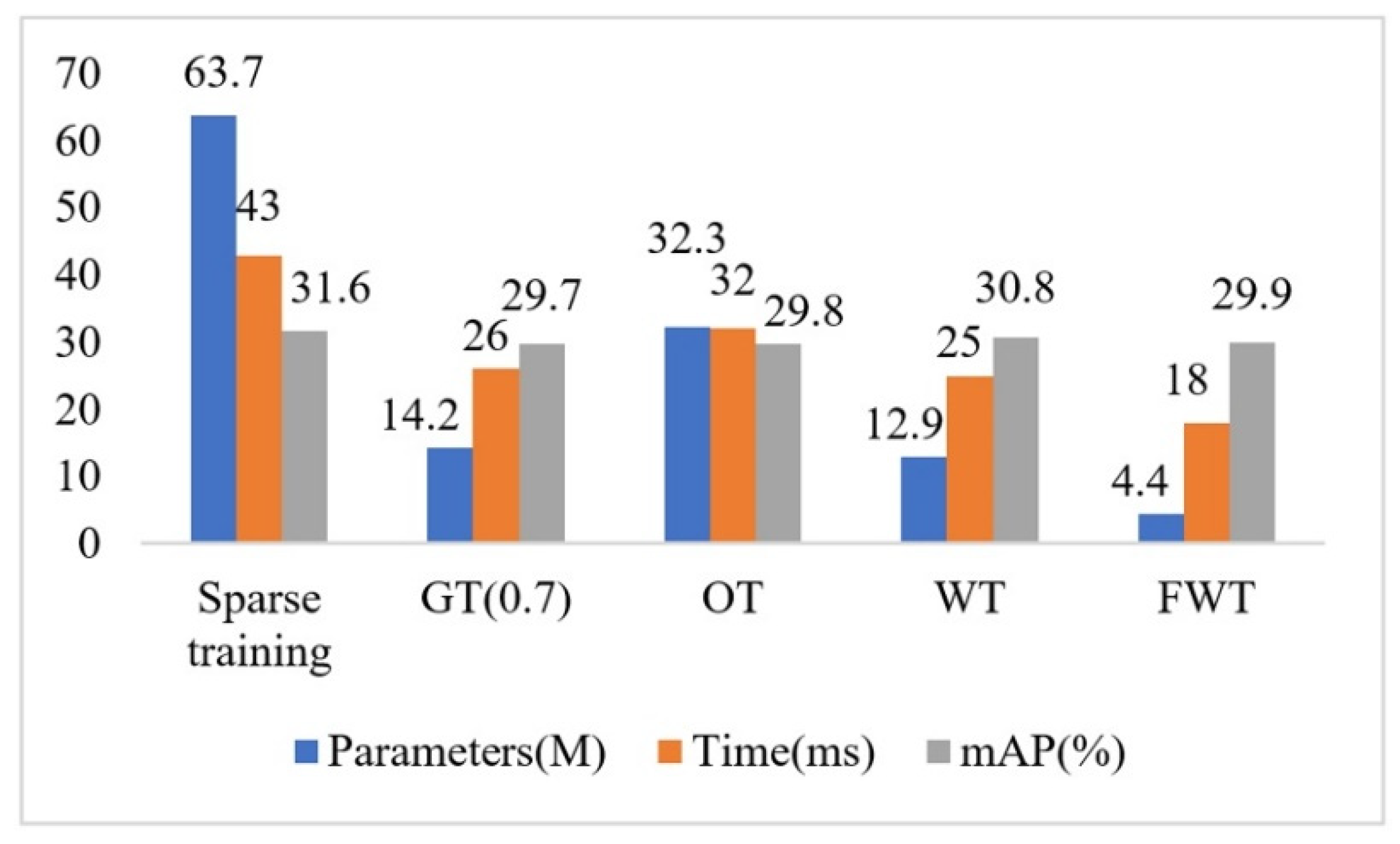
• We propose a more efficient channel pruning method for model compression, which can achieve higher detection efficiency for real-time detection and practical applications. Specifically, we can slim the network parameters from 63.7 million (M) to 3.3M, which decreases the parameter size by 94.8%. Theoretically, our proposed channel pruning idea could also be used for slimming the network model in other fields.

The rest part of this work is summarized as follows. Section 2 briefly reviews the most or some related works. In Section 3, we detail the proposed method. Section 4 illustrates the experimental datasets, procedures, and evaluation criteria. In Section 5, we verify the effectiveness of the proposed method, and compare the results on three public datasets. Finally, the discussions and conclusions of this paper are provided in Section 6 and Section 7.

2. Related Works

2.1. Multi-Scale Object Detection in Natural Scenes

In recent years, with the development of CNN, the object detection approaches based on deep learning have made significant progress. Generally, these approaches can be briefly divided into two categories: One- and two-stage detection approaches. To be specific, the two-stage approaches [2,26,27,28,29,30] first produce a set of region proposals, which are then optimized by CNN. Compared with one-stage approaches, they can usually achieve better positioning accuracy. Some of the most representative approaches are as follows. Faster R-CNN [2] optimizes the Fast R-CNN [26] by introducing the region proposal network (RPN), which can obtain the proposal regions from the feature maps through ROI-pooling [27]. R-FCN [28] builds a region-based fully convolutional network, while proposing the sensitive score maps with the position, which greatly promote the detection speed without affecting the detection precision. The unified multi-scale CNN (MS-CNN) [29] proposes a method for detecting multi-scale targets from multiple layers. Faster FPN [8] is a mainstream detector for detecting multi-scale objects, which designs a top-down structure for realizing the low-level features with more semantic information. The one-stage detectors [3,9,31,32,33,34] are generally faster in the detection speed because the predefined anchors can be directly classified and further refined without any step to generate proposals. In one-stage detection approaches, YOLOv2 [31] adopts multi-scale training via randomly electing a new image scale every few designated batches for making the network model realize the scale unchanged. DC-SPP-YOLO [32] adopts dense connection [35] and spatial pyramid pooling [16] to strengthen the multi-scale feature extraction on YOLOv2 [31]. The single-shot multi-box detector (SSD) approach [9] realizes different scale features through merging the multi-scale features of multiple levels without increasing the amount of calculation. Considering the severe category imbalance between the network foreground and background, RetinaNet [33] adopts the feature pyramid network and utilizes focal loss to tackle the defects of one-stage detection approaches. RefineDet [34] uses four feature extraction layers with different strides to handle the multi-scale objects. YOLOv3 [3] introduces a feature pyramid structure to detect the targets with multi-scale, and it is the baseline of the proposed network architecture.

2.2. Object Detection in Aerial Scenes

Since the objects in aerial images have various scales and shapes with a complex background, object detection in aerial images has become one of the most challenging problems [36,37]. In recent days, the object detection approach based on deep learning also shows its potential in the feature extraction and description of the remote sensing image. Due to the detection accuracy of the two-stage detection approach is usually superior to the one-stage detection approach, most aerial image object detection approaches focus on region-based object detection pipeline, namely, the two-stage detector. For instance, Ren et al. [38] adopted the idea of the deformable convolutional network [14] and proposed a two-stage network that could predict the rectangular bounding boxes and their categories in remote sensing images. Deng et al. [39] also built a two-stage detector that enhances the data by dividing the large-scale aerial images, and then fusing the same scale features of three levels to generate a new feature map. Ren et al. [40] used the structure of dense connection [35] to replace the commonly used FPN [8], and modified the default size of anchors, so it can make the network pay more attention to numerous small areas in the feature maps. Based on Faster R-CNN with FPN [8], Cheng et al. [41] designed an end-to-end cross-scale feature fusion (CSFF) framework to solve the problem of the large size difference and high similarity between target classes in remote sensing images. Yang et al. [42] constructed a remote sensing image object detector named SCRDet and used the attention mechanism to predict the rectangular rotation coordinates. Other studies [43] mainly used the multi-scale feature map fusion method to solve the problem of rapid change of target scale in aerial images. These approaches use different complex network structures to obtain high detection accuracy. But because the network models of these approaches are usually large and cannot meet the requirements of practical application, they are sub-optimal in the detection of multi-scale and multi-shape objects in aerial images. However, the one-stage detection approach has advantages in detection speed. Therefore, some researchers also study aerial image object detection based on the one-stage detection approach. For example, Tayara et al. [44] proposed a one-stage framework for aerial image object detection based on a densely connected convolutional network [35]. Sun et al. [4] designed an adaptive saliency-biased loss to improve the object detection performance in aerial images. You Only Look Twice (YOLT) [45], which is based on YOLOv2 [31], is a two-branch network that can predict the scene and target at the same time, and realize the rapid aerial image object detection. By improving YOLOv3 [3] framework, Ma et al. [46] realized significant improvement for locating collapsed buildings from post-earthquake remote sensing images, and Zhang et al. [47] proposed a scene-adaptive algorithm for vehicle detection in aerial images. These approaches generally obtain better detection efficiency for the multi-scale objects than the two-stage approaches. However, they are usually still relatively large and difficult to configure on the device for practical application.

2.3. Model Compression

To obtain good detection accuracy, a large network model is usually required. However, the large network models often have some redundant information, which affects the detection speed to some extent and makes it very difficult to deploy neural network model on resource-limited devices. Hence, various model compression methods are designed to produce more compact network models for practical application. The existing model compression methods can usually be described as follows: Low-rank decomposition (LRD) [48], pruning [19], quantization [49], knowledge distillation [50], and designing compact CNN [51]. For low-rank decomposition and quantization, they generally bring a relatively large decrease in accuracy, and quantization will produce a cartesian drift for deep networks. For knowledge distillation and designing compact CNN, they train the network model from scratch that requires many computing resources. Therefore, in this paper, we only discuss related work about pruning methods.

Pruning can remove the redundant weights and significantly reduce the complexity of the network, while not losing too much accuracy. Moreover, it is usually divided into structured pruning and unstructured pruning. The unstructured pruning [24] directly prunes unimportant channels without any constraint operations. Although this kind of method can obtain a certain effect after pruning, it usually requires special software or hardware devices, which limits the deployment of the pruned model on resource-limited devices. Technically, the unstructured pruning usually cannot be implemented directly in practice unless a software library or dedicated hardware is specifically designed for supporting the pruned models. Compared to the unstructured pruning, the structured pruning methods [19,20,21,22,23] are more likely to generate a regular and easy-to-handle network framework, which are easier to implement in many practical applications. Among the existing structured channel pruning methods, researchers usually design a predefined global threshold to determine which part of the channels to be discarded. For instance, Liu et al. [19] proposed a simple channel pruning method with the global threshold, which is called network slimming. Note that the scale factors of the batch normalization (BN) [25] layer are used as the channel scale factors which are employed to measure the importance degree of the channels, and for obtaining channel-wise sparsity, the network is trained by L1 regularization on the scale factors of BN layers. Based on [19], Zhang et al. [21] proposed a faster deep object detector and used small scale factors to prune the less important feature channels. He et al. [22] introduced a new channel pruning method by minimizing the reconstruction error on the output feature maps, which can accelerate the networks with less precision loss. Different from the above methods, Ye et al. [23] proposed an independent local optimal threshold for each pruning layer to prune less important channels. In a word, although these methods are very simple, their channel pruning thresholds either only consider the global importance distribution of all layers or only consider the local importance distribution of each channel in the corresponding each layer. Therefore, these methods still cannot achieve a completely efficient model pruning.

3. Proposed Method

3.1. Polymorphic and Group Attention Modules

3.1.1. Polymorphic Module

To detect the multi-scale objects, many advanced network modules [15,16,17] with multi-scale structures have been proposed and proved efficiently. With reasonable design, these modules can cover the multi-scale receptive fields and effectively increase the multi-scale feature extraction capability of neural networks. However, these modules only consider the multi-scale information of the targets, but not the huge difference of target shape information. As a result, the detection effects of these modules are usually not good enough for various aerial images with multi-shape and multi-scale objects under complex background. Therefore, to solve the above problems, this paper designs a structure called a polymorphic module (PM), as shown in Figure 3. In the designed PM, a four-branch structure is designed to extract the different spatial-wise features. Each branch pays attention to the different shape information, respectively, and meanwhile, inside each branch, the different receptive fields are adopted to enrich the information of the different scales. In this way, the different branches can effectively extract the features with multi-shape and multi-scale information, and the obtained different feature information from all branches can be shared with each other. To make it easier to describe the proposed module, we simply name these four branches in PM as G1 branch, G2 branch, G3 branch, and PWConv (pointwise convolutions, also called 1 × 1 convolutions) branch in sequence.

For the G1 branch, it consists of a G1 block and a 1 × 1 convolutional layer, where the 1 × 1 convolution can be utilized to control the output number of channels of the G1 branch to 1/4 of the input channels. For the G1 block, it comprises of a 1 × 1 convolutional layer and four streams. Inside the G1 block, to reduce the computational cost, we first use a 1 × 1 convolutional layer to reduce the number of channels to 1/4. Moreover, then, we design four parallel atrous convolutional layers of the different rates for obtaining the different scale receptive fields and achieving the different scale features with more details. The diverse dilation rates of these 3 × 3 atrous convolutional layers in G1 block are 1, 3, 5, and 7, respectively. When the dilation rate is 1, it is the normal 3 × 3 convolution. To reduce module parameters and calculations, all atrous convolutional layers employ depthwise convolutions (DWConv) [52], and we call atrous depthwise convolution as ADWConv. The details of ADWConv are shown in the purple dotted box in Figure 3. Different from the conventional convolution operations for which each convolution kernel operates all channels of the input feature map at the same time, a convolution kernel of ADWConv is responsible for one channel; that is, one channel is convolved by only one convolution kernel. Therefore, the parameter quantity and calculation cost of ADWConv are lower than conventional convolutions. However, due to ADWConv independently performs convolution operations on each channel of the input layer, it does not effectively use the feature information of the different channels in the same spatial position. Based on this, we design a 1 × 1 convolution after G1 block to integrate the information flow of the different channels because the 1 × 1 convolution can encode the relationship of channels.

For the G2 branch and G3 branch, except that the shape of the convolution kernel is different in four parallel ADWConv layers of the corresponding block, their basic structure is the same as the G1 branch. Particularly, for the G2 block, the parallel ADWConv layers use 1 × 3 atrous convolutions, and the diverse dilation rates are also 1, 3, 5, and 7, respectively. Hence, this block can effectively learn the feature information of the targets with hugely different shapes in the horizontal direction, and the aspect ratios of these targets are even vastly different in aerial images. In the same way, the G3 block can effectively learn about the target features that vary greatly in shape in the vertical direction. In addition, due to the design of different kernels in the G2 block and G3 block, the edge information of the targets can be better extracted.

Finally, a PWConv branch is used to preserve the original information. Since the output number of channels of each branch is set as 1/4 of the input channels, the numbers of input and output channels of the PM module are consistent through concatenating the four branches at last. In addition, because the center points of the different convolution kernels in PM are coincident, the PM is also able to make the network better concentrate on the key feature of the objects, which can achieve more accurate detection. The operations of PM can be calculated as (1).

$$\begin{gathered} C_{pw}=f\left(X\right)=\delta \left[BN\left(w_{1\times 1}\ast X\right)\right], C_1=f\left(S_{n-1}\right) \\ {G}_K=Cat[\mathrm{ADWConv}{\left(C_1\right)}_{K, R=1},\mathrm{ADWConv}{\left(C_1\right)}_{K, R=3},\mathrm{ADWConv}{\left(C_1\right)}_{K, R=5},\mathrm{ADWConv}{\left(C_1\right)}_{K, R=7}] \\ {C}_2=f\left(G_{K=3\times 1}\right), C_3=f\left(G_{K=1\times 3}\right), C_4=f\left(G_{K=3\times 3}\right) \\ {S}_n=Cat\left[C_1,C_2,C_3,C_4\right] \end{gathered}$$

(1)

where w and the subscripts of w are the weights and the size of the convolutional kernel, respectively. BN is the batch normalization [25], and δ is the leaky rectified liner unit (LeakyReLU) [53] function. R is the dilation rate, and K denotes the convolutional kernel. Cat represents the concatenation operation. $S_{n-1}$ and $S_n$ are the input and output features, respectively. Compared with using a conventional 3 × 3 convolution with 512 input and output channels for which the parameters are about 2.36 million (M), using the PM with the same channel takes fewer parameters, which are around 0.87M, but can learn richer information, including multi-shape and multi-scale object features for aerial images.

3.1.2. Group Attention Module

In general, the existing multi-target detectors [3,8] aggregate the different features of CNN to detect various objects by a simple summation or concatenation with the unified weights, which ignores the different importance of the different layers or channels. Channel attention [54] has proved that assigning the different weights to the different channels can effectively enhance useful features for neural networks and suppress unimportant features. In this work, based on such a consideration that the direct concatenation of multi-branch network structures ignores the different importance of each branch group, we devise a group attention module (GAM) for better utilizing the diversiform concatenation features in the network. Through the GAM module, each concatenate part can obtain a learned weight to optimize different concatenate features. The detail of the GAM is illustrated in Figure 4.

In the devised GAM, we define each branch of the concatenation operation as a group, and group*n denote that there are n groups in the concatenate feature maps. We assume that the combined feature maps consist of four branches (n = 4), as shown in Figure 4. For example, the proposed PM has four branches, and the concatenate feature maps are obtained by combining the different information of these four branch groups. In the GAM, inspired by the convolutional block attention module (CBAM) [55], both the max-pooling and the average-pooling are used to reduce the spatial dimension of the concatenate feature maps. Then the produced max-pooling and the average-pooling features are input to two weights-shared full convolutional layers. The hidden layer size and the output layer size both are the number of groups. Moreover, the output vectors of the weight-shared full convolutional layers are fused by the element-wise addition. After passing through a sigmoid function, the merged vector is multiplied by the original concatenate feature maps to obtain the weighted feature maps. Finally, we add a shortcut connection with the original feature maps to enhance information dissemination and produce the final weighted feature maps. The GAM module can be defined as (2).

$$\begin{gathered} F_{Max}=\left(w_{1\times 1}^2\ast \left(w_{1\times 1}^1\ast MaxPooling\left(F_{n-1}\right)+b_1\right)+b_2\right) \\ {F}_{Avg}=\left(w_{1\times 1}^2\ast \left(w_{1\times 1}^1\ast AvgPooling\left(F_{n-1}\right)+b_1\right)+b_2\right) \\ W={\mathsf{\delta }}_0\left(F_{Max}\oplus F_{Avg}\right) \\ {F}_n=\left(F_{n-1}\otimes W\right)\oplus F_{n-1} \end{gathered}$$

(2)

where ${\mathsf{\delta }}_0$ is the sigmoid function, w and b are the weights and bias, respectively. The subscript of w is the size of the convolutional kernel, and the superscript of w is the sequence number of the convolutional layer. $\oplus$ and $\otimes$ are the element-wise addition and element-wise multiplication, respectively. W is the weight of the group. $F_{n-1}$ is the concatenate feature maps for input and $F_n$ is the weighted feature maps for output.

3.2. PG-YOLO Detector

To make full use of the advantage of the proposed modules, we further propose a novel one-stage network called PG-YOLO, which embeds the polymorphic and group attention modules. Thus, the proposed PG-YOLO considers the huge difference in the target scale and that in the target shape of aerial images simultaneously. In addition, the PG-YOLO designs four detection headers with the adaptive anchors to achieve higher detection accuracy for multi-scale and multi-shape objects. The entire structure of PG-YOLO is shown in the orange box of Figure 5. Specifically, as depicted on the right side of Figure 5, the detection headers with low-resolution yet high-semantic information (y1 and y2) are mainly responsible for detecting large-scale targets, while the detection headers with high-resolution yet low-semantic information (y3 and y4) focus on detecting small-scale targets.

3.2.1. Multi-Detection Headers

For the PG-YOLO, we utilize Darknet-53 [3] as our backbone, which including 23 residual blocks, as shown in the dark green blocks of Figure 5. In addition, according to the characteristics of the data whose object sizes are widely distributed, we design four detection headers for better detecting the multi-scale objects compared to the original three detection headers. We display the size distributions of three public aerial datasets, including VisDrone-DET (vision meets drone object detection) [5], DIOR (object detection in optical remote sensing images) [1], and DOTA (a large-scale dataset for object detection in aerial images) [36] datasets in Figure 6.

From Figure 6, it can be seen clearly that the object size of VisDrone-DET dataset (Figure 6a) is widely distributed between 0 and 600 pixels, while that of the DIOR dataset (Figure 6b) is more widely distributed between 0 and 800 pixels. Moreover, for the DOTA dataset (Figure 6c), the images are chipped into 1024 × 1024 pixels, due to the large size of these images, and the object size is distributed between 0 and 1024 pixels. Hence, to detect objects of vastly different sizes mentioned above, we design multi-detection headers in the PG-YOLO, and the different detection headers can detect the objects with different scales. In particular, when the size of the input image is limited to 608 $\times$ 608 pixels, the final feature maps of these four detection headers are 19 $\times$ 19, 38 $\times$ 38, 76 $\times$ 76, and 152 $\times$ 152 pixels corresponding to the detection header 1, 2, 3, and 4, respectively.

3.2.2. Embedding the Polymorphic and Group Attention Modules

As can be seen in the red dotted box of Figure 5, the polymorphic module (PM) and group attention module (GAM) are integrated in front of the detection headers. Especially, the PM is inserted between the detection header 1 and the backbone to simultaneously learn multi-scale and multi-shape information of the targets. In the PG-YOLO, it concatenates the deep low-resolution features with high-semantic information and the shallow, high-resolution features with low-semantic information to fuse the different scale features and improve the multi-scale object detection capability. After the concatenation in the different detection headers (y1 and y2, y2 and y3, y3 and y4), we add the GAM to weigh the different scale features, and the number of groups of this GAM is 2 (GAM2). Besides, a GAM is also set after the PM to weigh various branch features, and this GAM after PM has four groups (GAM4), due to there are four branches in the PM.

3.2.3. Adaptive Anchors

In the PG-YOLO, some bounding box priors with fixed size (anchors) are set in the output feature map of the network, and the prediction box can be obtained through the mapping adjustment of the network learning parameters and the size of prior boxes. In this paper, we introduce the adaptive anchors for every dataset. In particular, we adopt the k-means algorithm with the intersection of union (IoU) distance [31] to obtain the adaptive anchors through clustering the object size of the training set in the corresponding dataset. For the VisDrone-DET dataset, the adaptive anchors are [(6,10), (10,21), (14,12), (17,31), (24,15), (27,49), (30,22), (41,37), (52,25), (55,76), (84,46), (129,109)]. Besides, for the DIOR dataset, the adaptive anchors are [(6,8), (11,27), (12,10), (17,18), (22,53), (28,12), (28,28), (48,19), (53,40), (64,85), (138,159), (348,356)]. At last, the adaptive anchors of DOTA dataset are [(14,15), (20,34), (29,42), (37,19), (38,90), (39,33), (45,47), (58,28), (65,71), (90,47), (99,104), (183,207)].

3.3. A More Efficient Channel Pruning Method

3.3.1. Sparsity Training

In this work, we propose a more efficient channel pruning method for model compression. Its simplified representation is shown in the blue box of Figure 5, with details as follows. The sparse training is the most important to obtain the coefficient of pruning layer for the structured pruning. Moreover, sparse training is the game process of precision and sparsity. We generally set a penalty factor to hold the model with high precision and achieve relatively high sparsity. In addition, the channel-wise sparsity in the network model is beneficial for channel pruning. To realize more efficient channel pruning, same as [19,23], a static scale factor is set for each channel, and the absolute value of the static scale factor indicates the importance of the channel. More specifically, in addition to the final layer of the detection header, each convolutional layer in our network model is followed by a BN layer for accelerating convergence and improving generalization. Therefore, the scale factor of the BN layer can be used as the scale factor of the channel of the corresponding convolutional layer. BN layers normalize convolutional features, as expressed in (3).

$$y_i={\gamma }_i\times \frac{x_i-\overline{x}}{\sqrt{{\sigma }^2+\epsilon }}+{\beta }_i$$

(3)

where $\overline{x}$ and ${\sigma }^2$ are the mean value and variance of the input features in the mini-batch, ${\gamma }_i$ and ${\beta }_i$ are the i-th scale factor and bias of the BN layer. The absolute value of the scale factor in the BN layer is directly used to measure the importance of each channel. To better identify important channels from less important channels, we adopt channel-wise sparsity training through using L1 regularization on the scale factors $\gamma$. The sparsity training loss function is given as (4).

$$L={\sum }_{\left(x,y\right)}l\left(f\left(x,w\right),y\right)+\mu \left({\sum }_{\gamma ϵ\mathsf{\Gamma }}f\left(\gamma \right)\right)$$

(4)

where (x, y) represents the training inputs and the corresponding ground truth targets, w is the trainable weights, $f\left(\gamma \right)=\left|\gamma \right|$ expresses L1-norm, $\mu$ indicates penalty factor which balances these two losses. The first sum-term corresponds to the normal training loss of our network, which is consistent with the baseline YOLOv3 [3].

3.3.2. Distributions of the Scale Factors and the Pruning Thresholds

The pruning threshold plays a crucial role in the performance of the network model after channel pruning. The existing methods designing the pruning threshold either only consider the global importance distribution of all layers and set a global threshold [19], or only consider the local importance distribution of the different channels of each layer and set an independent local optimal threshold [23] for each layer. In general, the mean value of the absolute value of the scale factors (gamma_mean) for each pruning layer is used to indicate the importance of this layer, and the distribution line chart of the gamma_mean is shown in Figure 7. As can be seen from Figure 7, the importance of the different layers changes.

In addition, for further analyzing the effect of the different pruning thresholds on each pruning layer, we draw the distribution diagram of the different thresholds in the same pruning layer in Figure 8.

The global threshold, which is set according to the value distribution of all scale factors, does not consider the specific value distribution of the local scale factors in each layer. On the one hand, it is difficult to set an appropriate global threshold corresponding to the pruning percentage for achieving efficient pruning. As an example, in the 31st pruning layer, as shown in Figure 8a, if we set the pruning percentage to 0.5 or 0.7, a small number of channels will be pruned and cause under-pruning, but if we set the pruning percentage to 0.8, too many channels will be pruned and cause over-pruning. Furthermore, sometimes all channels of some layers are pruned by the excessive global threshold, which will break the overall structure of the network. On the other hand, for a global threshold that has been set in advance, the pruning effects of the different layers are also different. For example, when the pruning percentage is 0.8, the global threshold corresponding to the 31st pruning layer (Figure 8a) is too high, which may lead to over-pruning, while the global threshold corresponding to the 60th pruning layer (Figure 8b) is slightly low, which may lead to under-pruning.

And the local optimal threshold, which is set according to the scale factors distribution of the corresponding each layer, ignores the global importance in all layers. Therefore, it cannot reach both the local optimality of each layer and the global optimality of all layers at the same time. For instance, the gamma_mean of the scale factors of the 30th and 32nd pruning layers are very low, as shown in Figure 7, thus the global representations of these layers are less important, and a larger threshold should be set to prune more redundant channels. However, from Figure 8c,d, we can see that the local optimal thresholds of these two layers are relatively small, which makes it difficult to achieve efficient pruning.

3.3.3. Layer-Wise Weighted Threshold for Channel Pruning

Based on the above analysis and considering the value distributions of both global and local scale factors [19,23], we propose a more appropriate layer-wise weighted threshold for channel pruning to reduce the model parameters, while maintaining the detection accuracy, which can slim the model and realize the faster object detection. Firstly, considering the value distribution of the local scale factors of each layer, we calculate the pruning threshold for each layer as (5).

$$\begin{gathered} {\gamma }_{ot}={\gamma }^{\prime }\in \mathsf{\Gamma } \\ s.t. {\sum }_{\gamma \in ℱ\left({\gamma }^{\prime }\right)}{\gamma }^2<\theta {\sum }_{\gamma \in \mathsf{\Gamma }}{\gamma }^2, {\gamma }^{\prime 2}+{\sum }_{\gamma \in ℱ\left({\gamma }^{\prime }\right)}{\gamma }^2\ge \theta {\sum }_{\gamma \in \mathsf{\Gamma }}{\gamma }^2, ℱ\left(x\right)=\{\gamma |\gamma \in \mathsf{\Gamma },\gamma <x\} \end{gathered}$$

(5)

where $\mathsf{\Gamma }$ is the set of all scale factors of each layer, $\theta$ is a negligible fraction and ${\gamma }_{ot}$ is the obtained pruning threshold corresponding to each layer. More specifically, when all scale factors of one layer are arranged in the ascending order, the first scale factor with a cumulative sum of squares larger than or equal to $\theta {\sum }_{\gamma \in \mathsf{\Gamma }}{\gamma }^2$ is defined as the local optimal threshold ${\gamma }_{ot}$ of each layer.

Secondly, considering the value distribution of the global scale factors of all pruning layers and to make the threshold of each pruning layer more reasonable and effective, we add a weight $\mathit{w}$ to the right of the inequality (5) in the process of calculating the local optimal threshold mentioned above, and propose a layer-wise weighted threshold for balancing both the global importance of all layers and the local importance of the different channels of each layer. The weight $\mathit{w}$ is calculated by:

$$\mathit{w}={(\frac{\frac{{\sum }_i^c\left|\gamma \right|}{c}}{\frac{{\sum }_j^l\frac{{\sum }_i^c\left|\gamma \right|}{c}}{l}})}^{-1}$$

(6)

where $\left|\gamma \right|$ denotes the absolute value of the scale factor, c represents the number of channels in the corresponding layer, and l expresses the number of all pruning layers. Concretely, we first average the absolute value of the scale factor $\left|\gamma \right|$ for each pruning layer to obtain the local mean value $\frac{{\sum }_i^c\left|\gamma \right|}{c}$ (gamma_mean) of each layer. Then, we average all local mean value $\frac{{\sum }_i^c\left|\gamma \right|}{c}$ to gain the global mean value $\frac{{\sum }_j^l\frac{{\sum }_i^c\left|\gamma \right|}{c}}{l}$ of all layers. We take the ratio of the local mean value $\frac{{\sum }_i^c\left|\gamma \right|}{c}$ to the global mean value $\frac{{\sum }_j^l\frac{{\sum }_i^c\left|\gamma \right|}{c}}{l}$ to express the weight of importance for each pruning layer. The greater the ratio mentioned above, the greater the importance of this layer, and a smaller threshold should be set to retain more channels in this more important layer. Thus, we finally invert the ratio of the local mean value $\frac{{\sum }_i^c\left|\gamma \right|}{c}$ to the global mean value $\frac{{\sum }_j^l\frac{{\sum }_i^c\left|\gamma \right|}{c}}{l}$ to obtain the final weight $\mathit{w}$ of each layer. Therefore, the proposed layer-wise weighted threshold ${\gamma }_{wt}$ for channel pruning can be denoted as (7).

$$\begin{gathered} {\gamma }_{wt}={\gamma }^{\prime }\in \mathsf{\Gamma } \\ s.t. {\sum }_{\gamma \in ℱ\left({\gamma }^{\prime }\right)}{\gamma }^2<\mathit{w}\times \theta {\sum }_{\gamma \in \mathsf{\Gamma }}{\gamma }^2, {\gamma }^{\prime }{}^2+{\sum }_{\gamma \in ℱ\left({\gamma }^{\prime }\right)}{\gamma }^2\ge \mathit{w}\times \theta {\sum }_{\gamma \in \mathsf{\Gamma }}{\gamma }^2 \\ ℱ\left(x\right)=\left\{\gamma \right|\gamma \in \mathsf{\Gamma },\gamma <x\} \end{gathered}$$

(7)

4. Experiments

4.1. Datasets

For proving the effectiveness of the proposed method, we execute the comparative experiments of object detection in aerial images on public VisDrone-DET [5], DIOR [1], and DOTA [36] datasets.

Table 1. The general information about VisDrone-DET, DIOR, and DOTA datasets.

Dataset	Size (Maximum)	Categories	Images	Instances	Year
VisDrone-DET	$2000\times 1500$	10	10.209	$2.5\times {10}^6$	2018
DIOR	$800\times 800$	20	23.463	192,472	2018
DOTA	$\mathrm{12,029}\times 5014$	15	2806	188,282	2018

lists the general information on these datasets. Noting that the size in Table 1 refers to the maximum size in the corresponding dataset.

VisDrone-DET dataset contains 10.209 images (6471 for training, 548 for validation, 1580 for testing, and 1610 in the test-dev subset) captured by the different heights with the different drones equipped with cameras across 14 different cities in China, which consists of 10 categories: Pedestrian, people, bicycle, car, van, truck, tricycle, awning-tricycle, bus, and motor. These images are annotated by more than 2.5 million bounding boxes of instances. Furthermore, the static images are obtained with different weather and lighting conditions, which is beneficial for enhancing the robustness of the model.

DIOR dataset covers 23.463 images with 192.472 instances. Moreover, it is divided into 20 categories: Airplane (APL), airport (AP), baseball field (BF), basketball court (BC), bridge (BR), chimney (CH), dam (DA), expressway service area (ESA), expressway toll station (ETS), golf course (GC), ground track field (GTF), harbor (HA), overpass (OP), ship (SH), stadium (SD), storage tank (ST), tennis court (TC), train station (TS), vehicle (VH), and windmill (WM). Each category has about 1200 images. DIOR reaches a great larger scale in categories, instances, and total images comparing to precious aerial datasets. The image size is 800 × 800 pixels in this dataset, and the range of spatial resolution is 0.5-30m. These images were obtained under different conditions, due to the variability of the weather, the season, and the quality of imaging equipment, so the specific contents are very different even if the image depicts the same place, which makes DIOR a more challenging task to detect. The annotation of DIOR is the horizontal bounding box. Besides, the distribution of training data and testing data are very close to ensure a good balance.

DOTA dataset consists of 2806 aerial images and 188.282 annotated object instances in 15 categories, which are plane (PL), baseball diamond (BD), bridge (BR), ground track field (GTF), small vehicle (SV), large vehicle (LV), ship (SH), tennis court (TC), basketball court (BC), storage tank (ST), soccer ball field (SBF), roundabout (RA), harbor (HA), swimming pool (SP), and helicopter (HC). The instances are annotated in two forms: The horizontal bounding boxes (HBB) and the oriented bounding boxes (OBB). Note that this work focuses on detecting the horizontal bounding boxes. Besides, for training and validation, the images are chipped into 1024 × 1024 pixels with an overlap value 200 pixels, due to the large size of these images.

4.2. Experimental Procedures

4.2.1. Normal Training

Following the training strategies provided by the Darknet [3] in PyTorch repository, our proposed detector is trained on an Nvidia GTX 1080Ti GPU with 11-GB RAM in an end-to-end manner, and the synchronized stochastic gradient descent (SGD) with a weight decay of 1e-4 and momentum of 0.9 is used to optimize our detector. When the input images are resized to 608 pixels for avoiding using much memory, the mini-batch is set to 7. But when the input size is 832 pixels to obtain higher accuracy, these are only four input images for each mini-batch. Note that for the DIOR and DOTA datasets, the input images are resized to 608 pixels in all experiments. We train a total of 200 epochs with a learning rate of 1e-3 for the first 140 epochs, 1e-4 for the next 40 epochs, and 1e-5 for the remaining 20 epochs.

4.2.2. Training with Sparsity

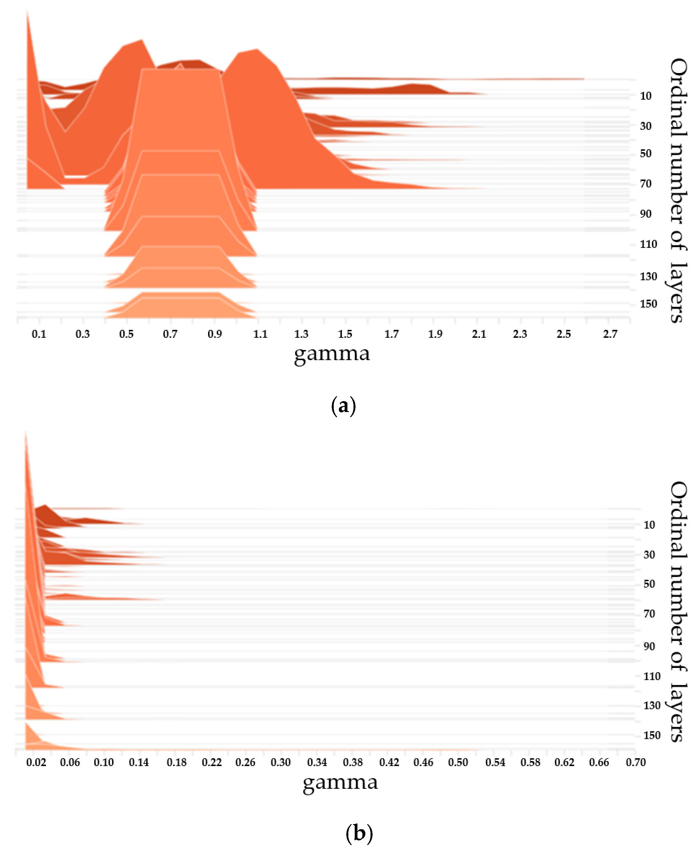
When our network model reaches the ideal precision, the sparse training with sparse channel regularization will be implemented. Specifically, we execute channel-wise sparsity training on the PG-YOLO for 200 epochs. Moreover, we choose the optimal penalty factor $\mu$ of the training loss function as 1e-3 in the experiments. Furthermore, the residual parameters of sparse training are the same as those in the normal training. In addition, the histograms of scale factors before and after sparse training are shown in Figure 9. In Figure 9, the vertical axis represents the ordinal number of the convolutional layer, and the horizontal axis represents the corresponding distribution of scale factors $\gamma$ (gamma) for each layer. As can be seen from Figure 9, after sparse training, the scale factor of the unimportant channel tends to be near zero, which is more conducive to channel pruning.

4.2.3. Pruning

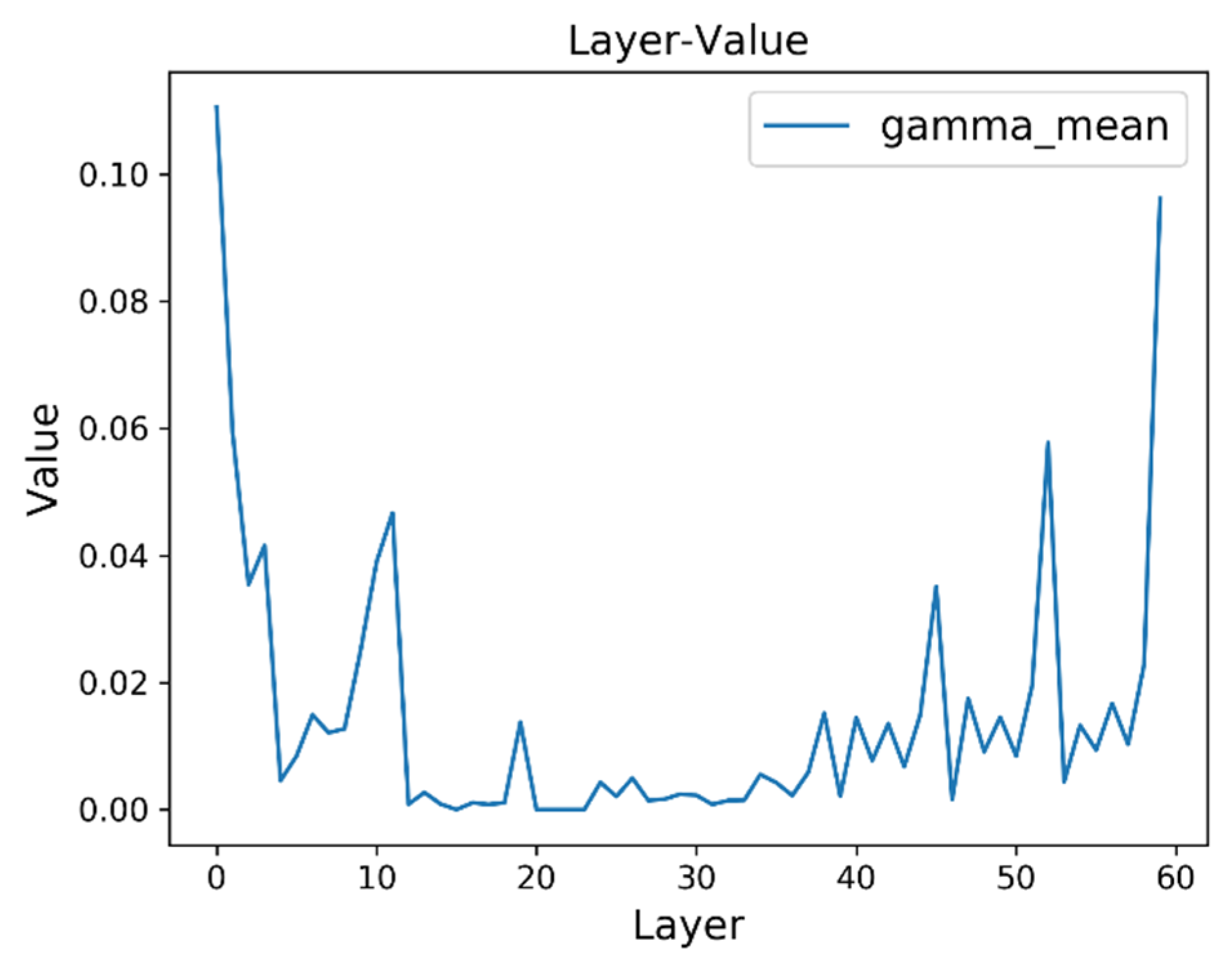
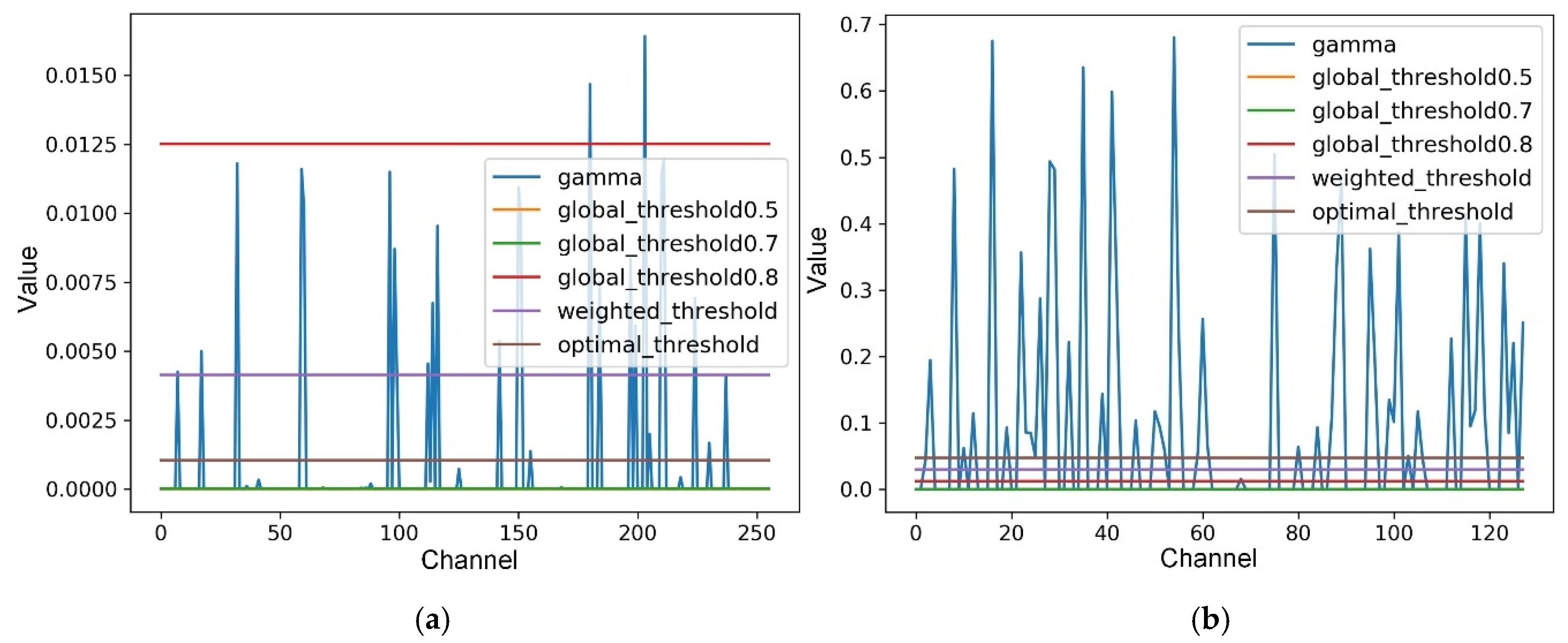
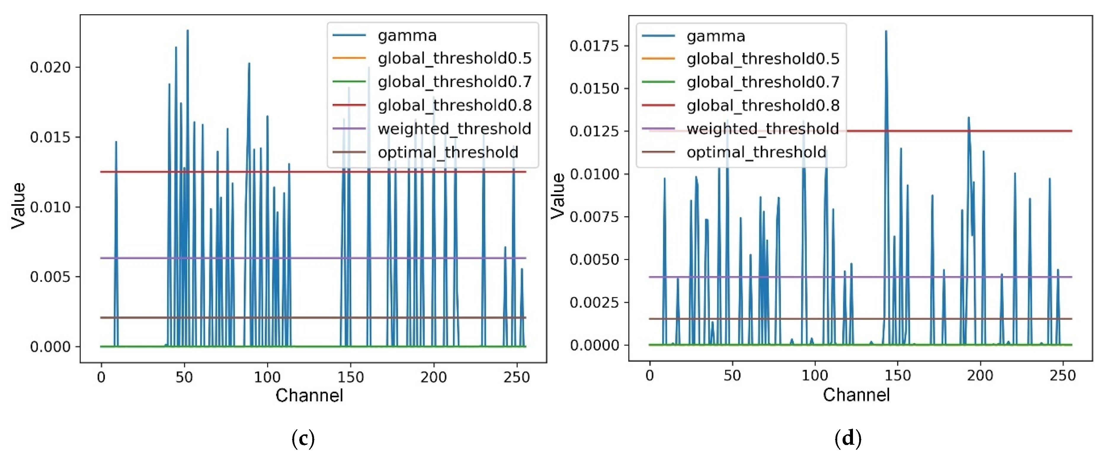
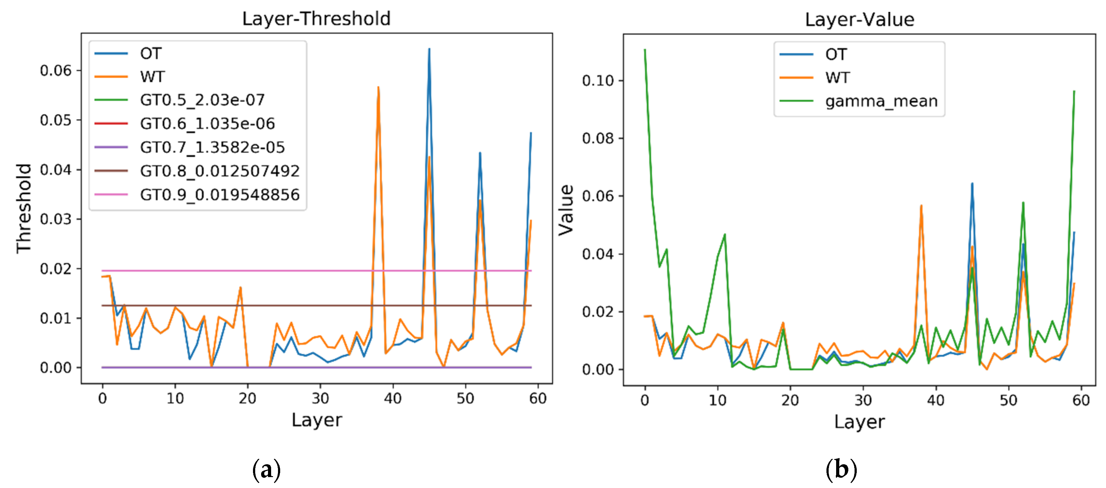
After sparsity training, we apply the proposed layer-wise weighted threshold for determining whether a channel should be pruned or not in each layer. Moreover, we set $\theta$ to 1e-4 in our experiments. Compared with [19], the proposed method cannot appear to prune all the channels of a layer, because our designed pruning threshold for each layer is reasonably distributed between the maximum and minimum values of scale factors. Especially, we generally utilize the normal pruning method, which ignores the convolutional layer of residual shortcut connection to execute channel pruning, because it usually has little effect on accuracy. In addition, for further reducing the unimportant parameters of the model, we also carry out extreme shortcut pruning for which the pruning layer include the convolutional layer of residual shortcut connection, and the pruning results are shown in Section 5.

4.2.4. Fine-Tuning

After channel pruning, the detection accuracy of the neural network model may be decreased. Therefore, we usually need to fine-tune the model after pruning to improve accuracy. It is worth noting that since our normal pruning has little impact on detection accuracy, we only fine-tune the model after extreme shortcut pruning. More specifically, the weights of the shortcut pruned PG-YOLO are used to initialize this slimmed network when fine-tuning, and other training hyper-parameters are the same as the normal training.

4.3. Evaluation Criteria

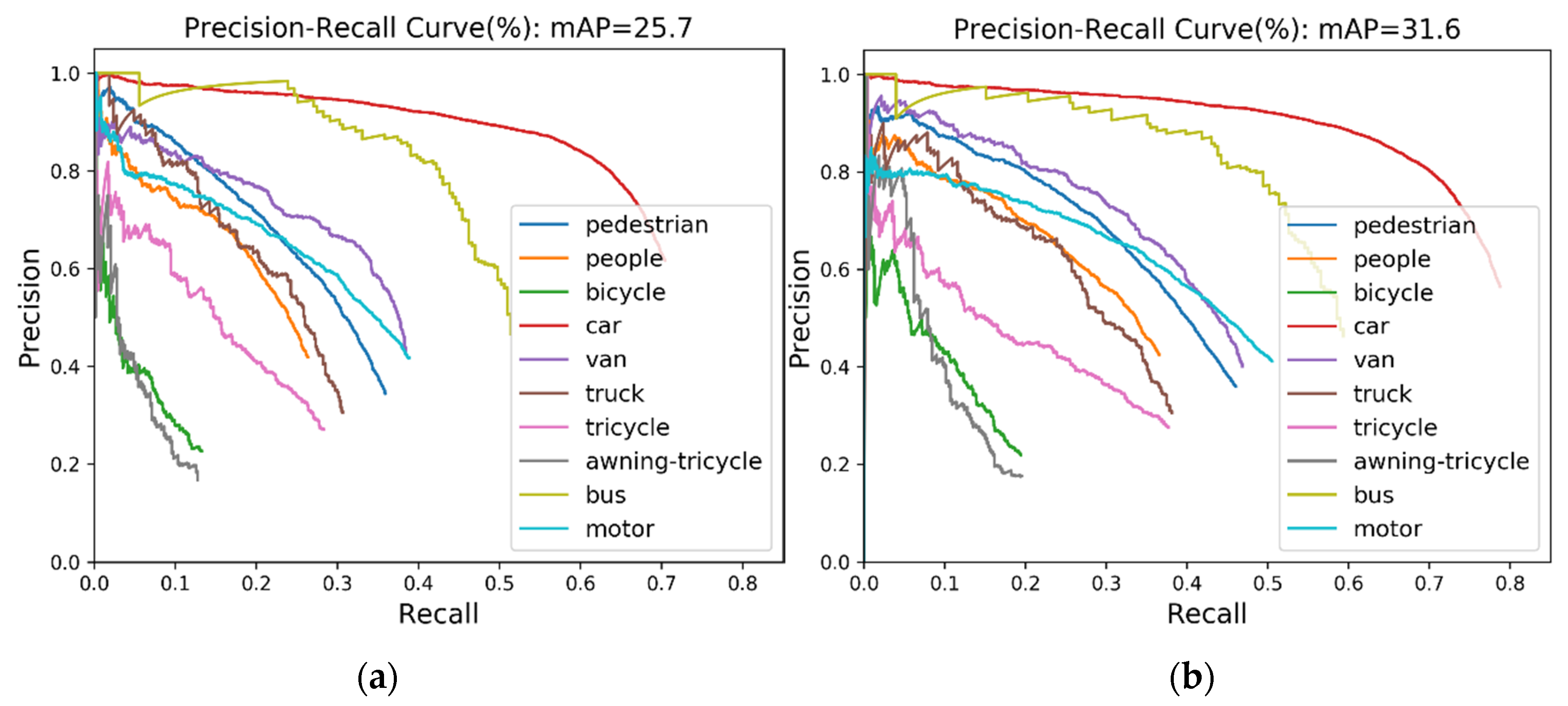
In this paper, to ensure the fairness of the experiments, the experimental data and the parameter settings are strictly consistent. In the experiments, the evaluation metrics used to quantitatively evaluate the model performance mainly include: (1) Precision, (2) recall, (3) F1 score, (4) mean average precision (mAP), (5) model parameters, (6) model volume, (7) compression rate (CR): The percentage of parameter reduction, (8) average run time per image, and (9) precision-recall curve (PRC).

The precision value, recall rate, and F1 score can be formulated as:

$$Precision=\frac{TP}{TP+FP}$$

(8)

$$Recall=\frac{TP}{TP+FN}$$

(9)

$$F1=\frac{2\times Precision\times Recall }{Precision+Recall}$$

(10)

where TP, FP, and FN represent the number of true positives, false positives, and false negatives, respectively. The PRC illuminates the correlation between precision and recall. When the particular detector maintains high precision with the increase of the recall rate, it is considered to be excellent in performance. The region area under the PRC is AP, which is the average precision of all recall values from 0 to 1. The mean average precision (mAP) represents the average precision value for all categories. It is worth noting that the higher the value of mAP, the better the performance of the detector.

5. Results

In this paper, we execute the ablation experiments on the VisDrone-DET validation dataset with an input size of 608 × 608 pixels. Furthermore, to further testify the effectiveness of the proposed method, we compare the proposed method with the other advanced methods on the VisDrone-DET, DIOR, and DOTA datasets. All experiments indicate clearly that the proposed method can effectively improve the performance of object detection in aerial images.

5.1. Ablation Experiments

5.1.1. Effect of the Polymorphic and Group Attention Modules

For verifying the effectiveness of the polymorphic module (PM), we perform the comparative experiment between the baseline model YOLOv3 [3] and the YOLOv3 with the PM (Y1), and the experimental results are displayed in the second and third rows of

Table 2. The comparison results for the proposed method and the baseline YOLOv3 on the VisDrone-DET validation dataset. PM, polymorphic module; GAM4, group attention module, which is located after the polymorphic module; GAM2, group attention module, which is located after the concatenation of two detection headers; AA, adaptive anchors; 4H, four detection headers. Y1, Y2, Y3, Y4 are the abbreviation of the models for which the PM, GAM4, GAM2, and AA are added to YOLOv3 in turn. PG-YOLO, the proposed model; ms, millisecond.

Method	PM	GAM4	GAM2	AA	4H	Time (ms)	mAP (%)
YOLOv3	-	-	-	-	-	35	25.7
Y1	√	-	-	-	-	38	26.9
Y2	√	√	-	-	-	39	27.2
Y3	√	√	√	-	-	41	28.7
Y4	√	√	√	√	-	41	29.8
PG-YOLO	√	√	√	√	√	43	31.6

. It can be seen that when adding the PM to the YOLOv3, the Y1 achieves comparable detection results as the baseline YOLOv3. With a little more inference run time, the Y1 outperforms YOLOv3 by 1.2% in mAP. This implies that the Y1 can help the detector to extract useful multi-scale and multi-shape features in high-resolution input images through the convolutional layers with the kernels of the different sizes and the different shapes.

In addition, we also visualize some feature maps generated by the YOLOv3 and Y1 at the same layer, as shown in Figure 10. Figure 10a is an example of input images, Figure 10b,c and Figure 10d–f are feature maps from the YOLOv3 and Y1, respectively. Although Figure 10b,c shows some multi-scale and multi-shape information, it is incomplete, such as missing the personal information or incomplete vehicle shape. From Figure 10d–f, because of the addition of the PM, it is obvious that the feature maps generated by the Y1 contain more multi-scale and multi-shape information, such as the people, the car, and the bus.

A more obvious demonstration is shown in Figure 11, which is the size distribution of the true positive detected objects by YOLOv3 (Figure 11a) and Y1 (Figure 11b). Furthermore, the key information of the target is more prominent for the feature maps of the Y1, due to the PM can also make the network focus better on the key feature of the objects.

In this paper, after the concatenation in the different detection headers, we add the group attention module (GAM) to weight the different scale features, and the number of groups of this GAM is 2 (GAM2). Besides, the GAM after PM has four groups (GAM4) because there are four branches in the PM. As shown in the fourth and fifth rows of Table 2, both Y2 (YOLOv3 with PM and GAM4) and Y3 (YOLOv3 with PM, GAM4, and GAM2) perform better than the Y1 (YOLOv3 only with the PM), increasing mAP by 0.3% and 1.8%, respectively. Besides, with the similar inference run time, Y2 and Y3 outperform the baseline YOLOv3, and increase the total mAP by 1.5% and 3%, respectively.

5.1.2. Effect of the PG-YOLO Detector

As shown in Table 2, the proposed model PG-YOLO outperforms the baseline YOLOv3 by 5.9% in the mAP. Compared with Y3, Y4 (Y3 with the adaptive anchors (AA)) increases the mAP by 1.1%, while the final PG-YOLO (Y3 with AA and the four detection headers (4H)) promotes the mAP by 2.9%. For a more detailed comparison of the proposed PG-YOLO and the baseline YOLOv3, we display specific results for each category in

Table 3. The comparison results for the proposed PG-YOLO and the baseline YOLOv3 on the VisDrone-DET validation dataset.

Method		YOLOv3				PG-YOLO
Class	Instances	Precision	Recall	F1	mAP (%)	Precision	Recall	F1	mAP (%)
pedestrian	8840	34.4	35.9	35.1	25.9	37.8	46.1	40.4	33.7
people	5120	41.9	26.4	32.4	18.5	43.9	36.5	39.3	25.7
bicycle	1290	22.6	13.3	16.7	5.4	22.7	19.4	20.6	8.8
car	14100	61.7	70.4	65.8	64.1	58.2	78.8	65.8	71.7
van	1980	43.2	38.5	40.7	29	43.6	46.8	43.2	35.9
truck	750	30.5	30.7	30.6	21.6	32.2	38.1	33.9	25.8
tricycle	1040	27.1	28.3	27.7	15.2	29.6	37.7	31.9	18.5
awning-tricycle	532	16.7	12.8	14.5	5.1	17.9	19.5	18.5	9.3
bus	251	46.6	51.4	48.9	46	48.9	59.4	52	52.4
motor	4890	41.8	38.9	40.3	26.3	42.5	50.5	45.4	34.2
all	38800	36.6	34.7	35.3	25.7	37.7	43.3	39.1	31.6

. As displayed in Table 3, for the bus that has a large aspect ratio, the proposed PG-YOLO improves mAP by 6.4% than YOLOv3 (mAP: 52.4% vs. 46%). Moreover, compared with YOLOv3, although the precision value of PG-YOLO has increased by a relatively small amount, the recall rate of PG-YOLO has been greatly improved by 8.6%. This indicates that the proposed method can detect more ground truth boxes.

Finally, we illustrate the precision-recall curves of the PG-YOLO and YOLOv3 in Figure 12. Figure 12 shows that as the recall rate increases, the precision of the proposed PG-YOLO decreases more slowly, which manifests that the proposed method has better detection performance.

5.1.3. Effect of the Proposed Layer-Wise Weighted Threshold

To further testify the validity of the proposed layer-wise weighted threshold (WT) in channel pruning, we compare the pruning results of the proposed WT with that of the global threshold (GT) [19] and the local optimal threshold (OT) [23] by the normal pruning method on VisDrone-DET validation dataset. The comparative results are shown in

Table 4. The performance comparison of the proposed WT with GT and OT on the VisDrone-DET validation dataset. Noting that the sparse training is executed on PG-YOLO. M, million; MB, megabyte; ms, millisecond; ST, sparse training; CR, compression rate.

Method		Parameters(M)	Volume(MB)	CR	Time (ms)	mAP(%)
ST		63.7	255.3	0%	43	31.6
GT [19]	0.5	24.6	98.4	61.4%	30	31.4
	0.6	18.9	75.7	70.3%	28	30.6
	0.7	14.2	56.9	77.7%	26	29.7
	0.8	11.3	45.4	82.3%	25	6.8
	0.9	9.5	38.4	85%	23	0
OT [23]		32.3	129.6	49.3%	32	29.8
WT		12.9	51.9	79.7%	25	30.8
FWT		4.4	17.9	93.1%	18	29.9

.

Note that the sparse training (ST) is executed on PG-YOLO. From Table 4, based on the compromise between the mAP and parameters, the proposed WT is superior to GT and OT. Specifically, compared with the OT, the improved mAP of the proposed WT is 1%, and the parameters reduction of the WT is 19.4M. Furthermore, to further reduce the parameters of the model, we also perform extreme shortcut pruning. After shortcut pruning, we fine-tune the model and use FWT to represent the pruning results after fine-tuning, as shown in the last line of Table 4. The results show that the model parameters of FWT can be reduced to 4.4M, which is decreased by 93.1%, and the mAP still remains at a high level. Moreover, it can be seen more intuitively in Figure 13 that our method achieves higher detection accuracy and faster detection speed than other advanced methods, and only retains fewer parameters.

Moreover, we further analyze the rationality and effectiveness of the proposed layer-wise weighted threshold method. We draw the threshold distributions of WT, OT, and multiple GT in the different pruning layers, as shown in Figure 14a. It can be seen that WT and OT can better match the characteristics of each layer to achieve more efficient pruning. In addition, we show the distribution of WT, OT, and the gamma_mean for each pruning layer in Figure 14b. It is worth noting that the greater the gamma_mean, the greater the importance of this layer, thus a smaller pruning threshold should be set to retain more channels in this layer, and vice versa. It can be seen from Figure 14b that the proposed WT can better fit the importance distribution of each pruning layer. For example, the gamma_mean in the 50th to 60th pruning layers are relatively large, as can be seen in Figure 14b. This indicates that these layers are more important, and the pruning threshold should be set smaller. From Figure 14b, the proposed WT is smaller than the OT in the 50th to 60th pruning layers, thus the designed WT is more appropriate. In addition, the gamma_mean is very small near the 30th layer, which indicates that these layers are less important, and the pruning threshold should be set larger. From Figure 14b, the proposed WT is larger than the OT in these pruning layers. Therefore, the proposed layer-wise threshold method is more reasonable and effective.

5.2. Results on the VisDrone-DET Dataset

We compare the proposed PG-YOLO with other YOLOv3-based methods on the VisDrone-DET validation dataset, and the comparison results are displayed in

Table 5. The comparison results for the proposed method and other YOLOv3-based methods on the VisDrone-DET validation dataset with an input size of 608 × 608 pixels.

Method	Input Size	Parameters (M)	Time (ms)	mAP (%)
YOLOv3-tiny [3]	608	8.7	12.5	9.1
YOLOv3-SPP1 [21]	608	62.6	38.6	22.9
YOLOv3-SPP3	608	63.9	43.1	23.3
SlimYOLOv3-SPP3-50	608	20.8	25.6	22.6
SlimYOLOv3-SPP3-90	608	8	25.1	20.6
SlimYOLOv3-SPP3-95	608	5.1	24.1	19.1
PG-YOLO	608	63.7	43	31.6
WT-PG-YOLO	608	12.9	25	30.8
FWT-PG-YOLO	608	4.4	18	29.9

and

Table 6. The comparison results for the proposed method and other YOLOv3-based methods on the VisDrone-DET validation dataset with an input size of 832 × 832 pixels.

Method	Input Size	Parameters (M)	Time (ms)	mAP (%)
YOLOv3-tiny [3]	832	8.7	19.4	11
YOLOv3-SPP1 [21]	832	62.6	67.9	25.5
YOLOv3-SPP3	832	63.9	72.1	26.4
SlimYOLOv3-SPP3-50	832	20.8	44.1	25.8
SlimYOLOv3-SPP3-90	832	8.0	41.4	23.9
SlimYOLOv3-SPP3-95	832	5.1	24.1	19.1
PG-YOLO	832	63.7	71	40
WT-PG-YOLO	832	10.1	42	39.1
FWT-PG-YOLO	832	3.3	24	37.5

. YOLOv3-SPP [21] includes YOLOv3-SPP1 and YOLOv3-SPP3, as detailed in Reference [21]. From Table 5, it is obvious that the proposed PG-YOLO obtains the best results compared with YOLOv3-SPP1 and YOLOv3-SPP3 when the input size is limited to 608 × 608 pixels to avoid using too much memory. We use WT-PG-YOLO and FWT-PG-YOLO to simply represent the pruned models by the proposed WT and FWT on the PG-YOLO, respectively. In addition, there are three compressed models in Reference [21]: SlimYOLOv3-SPP3-50, SlimYOLOv3-SPP3-90, and SlimYOLOv3-SPP3-95. As shown in Table 5, compared with the minimum parameter compression model SlimYOLOv3-SPP3-95, the proposed FWT-PG-YOLO increases mAP by 10.8% with lower parameters and run time. Besides, with a little more inference run time, but lower parameters, the FWT-PG-YOLO outperforms YOLOv3-tiny [3] by 20.8% in mAP.

Moreover, to obtain higher detection accuracy, we increase the input size to 832 × 832 pixels, while the mAP of the PG-YOLO is increased to 40%, as shown in Table 6. Without fine-tuning, the proposed WT-PG-YOLO can prune the model from 63.7M to 10.1M by normal pruning. After extreme shortcut pruning and fine-tuning, the model parameters of the proposed FWT-PG-YOLO can be reduced from 63.7M to 3.3M, which is decreased by 94.8%, and the mAP still holds on the high level. Finally, we show the visualization effect of the PG-YOLO in Figure 15. As can be seen from Figure 15, although some small targets with a high coincidence degree, such as one or several people on a motor or tricycle, are partially missed, most of the targets can be correctly detected.

5.3. Results on the DIOR Dataset

To further testify the effectiveness of the proposed method, we also compare the proposed method with other advanced methods on the DIOR testing dataset. The categories are briefly represented in the middle of the first line in

Table 7. The comparison results for the proposed method and other advanced methods on the DIOR dataset. The categories are briefly represented in the middle of the first line, and the corresponding full names are in Section 4.1.

Method	Backbone	APL	AP	BF	BC	BR	CH	DA	ESA	ETS	GC	mAP (%)
		GTF	HA	OP	SH	SD	ST	TC	TS	VH	WM
RICAOD [56]	VGG16	42.2	69.7	62	79	27.7	68.9	50.1	60.5	49.3	64.4	50.9
		65.3	42.3	46.8	11.7	53.5	24.5	70.3	53.3	20.4	56.2
RIFD-CNN [57]	VGG16	56.6	53.2	79.9	69	29	71.5	63.1	69	56	68.9	56.1
		62.4	51.2	51.1	31.7	73.6	41.5	79.5	40.1	28.5	46.9
Faster R-CNN [2]	VGG16	53.6	49.3	78.8	66.2	28	70.9	62.3	69	55.2	68	54.1
		56.9	50.2	50.1	27.7	73	39.8	75.2	38.6	23.6	45.4
SSD [9]	VGG16	59.5	72.7	72.4	75.7	29.7	65.8	56.6	63.5	53.1	65.3	58.6
		68.6	49.4	48.1	59.2	61	46.6	76.3	55.1	27.4	65.7
YOLOv3 [3]	Darknet-53	72.2	29.2	74	78.6	31.2	69.7	26.9	48.6	54.4	31.1	57.1
		61.1	44.9	49.7	87.4	70.6	68.7	87.3	29.4	48.3	78.7
Faster R-CNN with FPN [8]	ResNet-50	54.1	71.4	63.3	81	42.6	72.5	57.5	68.7	62.1	73.1	63.1
		76.5	42.8	56	71.8	57	53.5	81.2	53	43.1	80.9
Mask-RCNN with FPN [58]	ResNet-50	53.8	72.3	63.2	81	38.7	72.6	55.9	71.6	67	73	63.5
		75.8	44.2	56.5	71.9	58.6	53.6	81.1	54	43.1	81.1
PANet [59]	ResNet-50	61.9	70.4	71	80.4	38.9	72.5	56.6	68.4	60	69	63.8
		74.6	41.6	55.8	71.7	72.9	62.3	81.2	54.6	48.2	86.7
CornerNet [60]	Hourglass-104	58.8	84.2	72	80.8	46.4	75.3	64.3	81.6	76.3	79.5	64.9
		79.5	26.1	60.6	37.6	70.7	45.2	84	57.1	43	75.9
PG-YOLO	Darknet-53	71.5	74.8	75.3	87.8	34.6	72	42	66.2	68.5	61.9	65.4
		62.6	49.8	49.1	88.8	66.6	73.2	87	44.3	49.1	82.8

, and the details of the category information are in Section 4.1. From Table 7, the proposed method achieves the optimal performance, which exceeds the YOLOv3 [3], SSD [9], Faster R-CNN [2] by 8.3%, 6.8%, 11.3% at mAP, respectively. For the objects with large aspect ratio in aerial images, such as airports and bridges (indicated as AP and BR in Table 7), our method PG-YOLO remarkably outperforms the YOLOv3 at mAP (airports: 74.8% vs. 29.2%. bridges: 34.6% vs. 31.2%), due to its stronger multi-scale and multi-shape information extraction ability. The visual detection results of the proposed method on the DIOR testing dataset are shown in Figure 16. From Figure 16, it can be clearly seen that the proposed method can achieve an excellent detection effect for both small size targets and large size targets.

5.4. Results on the DOTA Dataset

Furthermore, we also compare the related methods with the proposed method on the validation set of the DOTA dataset [36], and the comparison results are shown in

Table 8. The comparison results for the proposed method and other advanced methods on the DOTA dataset. The abbreviations in the middle of the first line indicate the categories, and the corresponding full names are in Section 4.1.

Method	PL	BD	BR	GTF	SV	LV	SH	TC	mAP (%)
	ST	SBF	RA	HA	SP	HC	ST
R-FCN [28]	81.0	58.9	31.6	58.9	49.7	45.0	49.2	68.9	52.5
	52.0	67.4	41.8	51.4	45.1	53.3	33.8
Faster R-CNN [2]	80.3	77.5	32.8	68.1	53.6	52.4	50.0	90.4	60.64
	75.0	59.5	57	49.8	61.6	56.4	41.8
SSD [9]	57.8	32.7	16.1	18.6	0.05	36.9	24.7	81.1	29.86
	25.1	47.4	11.2	31.5	14.1	9.09	0
YOLOv2 [31]	76.9	33.8	22.7	34.8	38.7	32.0	52.3	61.6	39.2
	48.5	33.9	29.2	36.8	36.4	38.2	11.6
R-FCN [28] with FPN	86.9	62.1	42.1	50.8	42.3	74.5	77.2	84.7	57.14
	53.0	60.7	43.1	42.7	64.9	46.9	24.6
Faster R-CNN with FPN [8]	86.6	61.9	43.3	49.5	47.3	76.4	71.1	85.3	57.72
	53.2	60.9	38.8	41.1	70.5	47.9	31.5
HyNet(Hy-32-ResNet-50) [61]	86.8	58.7	43.6	54.0	64.3	80.4	87.8	85.1	62.1
	53.8	60.3	41.7	47.6	76.5	48.6	40.3
PG-YOLO	91.8	72.1	45	54.5	76.3	78.6	87.2	91.6	69.1
	66	74.8	47.9	61.9	79.9	56.9	51.4

. The abbreviations in the middle of the first line in Table 8 indicate the categories, and the corresponding full names are in Section 4.1. From Table 8, it is notably shown that the proposed method possesses better performance. For the bridges (BR) and harbors (HA) that have a special shape and large aspect ratio in aerial images, the proposed PG-YOLO can obtain higher mAP, which is thanks to the advanced polymorphic module (PM), specifically designed for this situation in this work. Moreover, for small objects, such as planes (PL) and small vehicles (SV)), the proposed method can also achieve an effective detection effect. Finally, to better demonstrate the detection performance of the proposed method, we visualize part of the detection results, as displayed in Figure 17. As can be seen from Figure 17, even if there are a large number of targets with large scale and shape differences, as well as many small targets with dense distribution in the DOTA dataset, the method proposed in this paper is also able to achieve an excellent detection effect.

6. Discussion

By analyzing the characteristics of the objects concretely in arial images, this paper proposes an effective network PG-YOLO to improve the object detection accuracy of arial images. Based on the proposed network, we further propose an effective channel pruning method with the layer-wise weighted threshold to compress the network model to further reduce the model parameters and improve the detection speed. The design of the layer-wise weighted threshold both considers the global scale factors distribution of all layers and the local scale factors distribution of each layer, which means the proposed layer-wise weighted threshold integrates the importance distribution of each layer and the importance distribution of each channel in each layer. Therefore, the proposed channel pruning method is more reasonable and efficient when pruning the unimportant channels, and it can slim the model, while keeping high detection accuracy. The effectiveness of each component of the proposed method is proved by the ablation experiments. Especially, without fine-tuning, we can prune the model from 63.7M to 10.1M by the normal pruning on the VisDrone-DET dataset with the input size of 832 × 832 pixels. Moreover, after the extreme shortcut pruning with fine-tuning, the model parameters can be reduced from 63.7M to 3.3M, which decreases parameter size by 94.8%.

In addition, the proposed layer-wise weighted threshold for channel pruning can not only be applied to the object detection network proposed in this paper, but also the scholars in other fields can use it to compress their network models to reduce the model parameters and increase the model inference speed for practical application, such as classification, segmentation, etc. Although our method achieves higher object detection accuracy and the detection speed is also very fast, especially after the channel pruning for model compression, the methods with the baseline YOLOv3 have a common problem; that is, to pursue faster detection speed, it usually causes a certain degree of the detection accuracy loss. In the future, our work will focus on further improving detection accuracy, while maintaining a fast detection speed.

7. Conclusions

In this paper, to enable the network focus better on the key feature of the objects and achieve more accurate detection, we designed a polymorphic module (PM) to learn the diversity of object scales and shapes in aerial images. In addition, a group attention module (GAM) was designed to assign different importance to the different concatenation layers, which can better utilize diverse concatenation features. By embedding the designed two modules and devising multiple detection headers with adaptive anchors, we proposed a one-stage network called PG-YOLO for more reasonably extracting object features and realizing the higher detection accuracy of multi-scale and multi-shape objects. Furthermore, an efficient layer-wise weighted threshold in channel pruning was proposed for compressing the network model and realizing the faster object detection nearly without accuracy loss. Extensive comparative experiments were performed on three public aerial datasets, and the results proved that the proposed method significantly or distinctly outperforms the state-of-the-art methods.

References

1. Li, K.; Wan, G.; Cheng, G.; Meng, L. Object detection in optical remote sensing images: A survey and a new benchmark. ISPRS J. Photogramm. Remote Sens. 2020, 159, 296–307. [Google Scholar] [CrossRef]
2. Ren, S.; He, K.; Girshick, R.; Sun, J. Faster R-CNN: Towards Real-Time Object Detection with Region Proposal Networks. IEEE Trans. Pattern Anal. Mach. Intell. 2017, 39, 1137–1149. [Google Scholar] [CrossRef] [PubMed] [Green Version]
3. Redmon, J.; Farhadi, A.J. Yolov3: An incremental improvement. arXiv 2018. e-prints. [Google Scholar]
4. Sun, P.; Chen, G.; Geoence, Y.S.R. Adaptive Saliency Biased Loss for Object Detection in Aerial Images. IEEE Trans. Geosci. Remote Sens. 2020, 58, 1–12. [Google Scholar] [CrossRef]
5. Zhu, P.; Wen, L.; Bian, X.; Ling, H.; Hu, Q.J. Vision meets drones: A challenge. arXiv 2018, arXiv:1804.07437. [Google Scholar]
6. Adelson, E.H.; Anderson, C.H.; Bergen, J.R. Pyramid methods in image processing. RCA Eng. 1984, 29, 33–41. [Google Scholar]
7. Krizhevsky, A.; Sutskever, I.; Hinton, G.E. ImageNet classification with deep convolutional neural networks. In Proceedings of the International Conference on Neural Information Processing Systems (NIPS), Lake Tahoe, NV, USA, 3–8 December 2012; pp. 1097–1105. [Google Scholar]
8. Lin, T.Y.; Dollár, P.; Girshick, R.; He, K.; Hariharan, B.; Belongie, S. Feature pyramid networks for object detection. arXiv 2017, arXiv:1612.03144. [Google Scholar]
9. Liu, W.; Anguelov, D.; Erhan, D.; Szegedy, C.; Fu, C.; Berg, A.C. SSD: Single Shot Multibox Detector. In Proceedings of the European Conference on Computer Vision, Amsterdam, The Netherlands, 8–16 October 2016; pp. 21–37. [Google Scholar]
10. Li, Y.; Chen, Y.; Wang, N.; Zhang, Z. Scale-Aware Trident Networks for Object Detection. In Proceedings of the International Conference on Computer Vision (ICCV), Venice, Italy, 22–23 June 2020. [Google Scholar]
11. Qiu, H.; Li, H.; Wu, Q. A2RMNet: Adaptively aspect ratio multi-scale network for object detection in remote sensing images. Remote Sens. 2019, 11, 1594. [Google Scholar] [CrossRef] [Green Version]
12. Xu, Z.; Xu, X.; Wang, L.; Yang, R. Deformable ConvNet with Aspect Ratio Constrained NMS for Object Detection in Remote Sensing Imagery. Remote Sens. 2017, 9, 1312. [Google Scholar] [CrossRef] [Green Version]
13. Yan, J.; Wang, H.; Yan, M. IoU-adaptive deformable R-CNN: Make full use of IoU for multi-class object detection in remote sensing imagery. Remote Sens. 2019, 11, 286. [Google Scholar] [CrossRef] [Green Version]
14. Dai, J.; Qi, H.; Xiong, Y. Deformable convolutional networks. In Proceedings of the IEEE International Conference on Computer Vision, Venice, Italy, 22–29 October 2017; pp. 764–773. [Google Scholar]
15. Szegedy, C.; Vanhoucke, V.; Ioffe, S.; Shlens, J. Rethinking the inception architecture for computer vision. In Proceedings of the IEEE Conference on Computer Vision and Pattern Recognition, Las Vegas, NV, USA, 27–30 June 2016; pp. 2818–2826. [Google Scholar]
16. Xie, S.; Girshick, R. Aggregated Residual Transformations for Deep Neural Networks. In Proceedings of the IEEE Conference on Computer Vision and Pattern Recognition (CVPR), Honolulu, HI, USA, 22–25 July 2017. [Google Scholar]
17. Chen, L.-C.; Papandreou, G.; Kokkinos, I.; Murphy, K.; Yuille, A.L. Deeplab: Semantic image segmentation with deep convolutional nets, atrous convolution, and fully connected crfs. IEEE Trans. Pattern Anal. Mach. Intell. 2018, 40, 834–848. [Google Scholar] [CrossRef] [PubMed]
18. Liu, S.; Huang, D. Receptive field block net for accurate and fast object detection. In Proceedings of the European Conference on Computer Vision (ECCV), Munich, Germany, 8–14 September 2018; pp. 385–400. [Google Scholar]
19. Liu, Z.; Li, J.; Shen, Z.; Huang, G. Learning efficient convolutional networks through network slimming. In Proceedings of the IEEE International Conference on Computer Vision, Venice, Italy, 22–29 October 2017; pp. 2736–2744. [Google Scholar]
20. Ye, J.; Lu, X.; Lin, Z. Rethinking the smaller-norm-less-informative assumption in channel pruning of convolution layers. arXiv 2018, arXiv:1802.00124. [Google Scholar]
21. Zhang, P.; Zhong, Y.; Li, X. SlimYOLOv3: Narrower, Faster and Better for Real-Time UAV Applications. In Proceedings of the IEEE International Conference on Computer Vision Workshops, Long Beach, CA, USA, 16–20 June 2019; pp. 37–45. [Google Scholar]
22. He, Y.; Zhang, X.; Sun, J. Channel pruning for accelerating very deep neural networks. In Proceedings of the IEEE International Conference on Computer Vision, Venice, Italy, 22–29 October 2017; pp. 1389–1397. [Google Scholar]
23. Ye, Y.; You, G.; Zhu, X.; Yang, Q. Channel Pruning via Optimal Thresholding. arXiv 2020, arXiv:2003.04566. [Google Scholar]
24. Han, S.; Pool, J.; Tran, J.; Dally, W. Learning both weights and connections for efficient neural network. Adv. Neural Inf. Process. Syst. 2015, 1, 1135–1143. [Google Scholar]
25. Ioffe, S.; Szegedy, C.J. Batch normalization: Accelerating deep network training by reducing internal covariate shift. arXiv 2015, arXiv:1502.03167. [Google Scholar]
26. Girshick, R. Fast R-CNN. In Proceedings of the IEEE International Conference on Computer Vision, Santiago, Chile, 11–18 December 2015; pp. 1440–1448. [Google Scholar]
27. Girshick, R.; Donahue, J.; Darrell, T.; Malik, J. Region-Based Convolutional Networks for Accurate Object Detection and Segmentation. IEEE Trans. Pattern Anal. Mach. Intell. 2015, 38, 142–158. [Google Scholar] [CrossRef]
28. Dai, J.F.; Li, Y.; He, K.M.; Sun, J. R-FCN: Object Detection via Region-based Fully Convolutional Networks. arXiv 2016, arXiv:1606.06409. [Google Scholar]
29. Cai, Z.; Fan, Q.; Feris, R.S. A unified multi-scale deep convolutional neural network for fast object detection. In Proceedings of the European Conference on Computer Vision, Amsterdam, The Netherlands, 8–16 October 2016; pp. 354–370. [Google Scholar]
30. Song, G.; Liu, Y.; Wang, X.J. Revisiting the Sibling Head in Object Detector. In Proceedings of the IEEE/CVF Conference on Computer Vision and Pattern Recognition 2020, Seattle, WA, USA, 13–19 June 2020. [Google Scholar]
31. Redmon, J.; Farhadi, A. YOLO9000: Better, faster, stronger. In Proceedings of the IEEE Conference on Computer Vision and Pattern Recognition, Honolulu, HI, USA, 22–25 July 2017; pp. 7263–7271. [Google Scholar]
32. Huang, Z.; Wang, J.; Fu, X.; Yu, T.; Guo, Y. DC-SPP-YOLO: Dense connection and spatial pyramid pooling based YOLO for object detection. Inf. Sci. 2020, 522, 241–258. [Google Scholar] [CrossRef] [Green Version]
33. Lin, T.Y.; Goyal, P.; Girshick, R. Focal loss for dense object detection. In Proceedings of the IEEE International Conference on Computer Vision, Venice, Italy, 22–29 October 2017; pp. 2980–2988. [Google Scholar]
34. Zhang, S.; Wen, L.; Bian, X. Single-shot refinement neural network for object detection. In Proceedings of the IEEE Conference on Computer Vision and Pattern Recognition, Salt Lake City, UT, USA, 18–22 June 2018; pp. 4203–4212. [Google Scholar]
35. Huang, G.; Liu, Z.; Van Der Maaten, L.; Weinberger, K.Q. Densely connected convolutional networks. In Proceedings of the IEEE Conference on Computer Vision and Pattern Recognition, Honolulu, HI, USA, 21–26 July 2017; pp. 4700–4708. [Google Scholar]
36. Xia, G.S.; Bai, X.; Ding, J. DOTA: A Large-scale Dataset for Object Detection in Aerial Images. arXiv 2017, arXiv:1711.10398. [Google Scholar]
37. Guo, W.; Li, W.; Gong, W. Extended Feature Pyramid Network with Adaptive Scale Training Strategy and Anchors for Object Detection in Aerial Images. Remote Sens. 2020, 12, 784. [Google Scholar] [CrossRef] [Green Version]
38. Ren, Y.; Zhu, C.; Xiao, S. Deformable Faster R-CNN with Aggregating Multi-Layer Features for Partially Occluded Object Detection in Optical Remote Sensing Images. Remote Sens. 2018, 10, 1470. [Google Scholar] [CrossRef] [Green Version]
39. Deng, Z.; Hao, S.; Zhou, S.; Zhao, J. Toward Fast and Accurate Vehicle Detection in Aerial Images Using Coupled Region-Based Convolutional Neural Networks. Remote Sens. 2017, 10, 1–13. [Google Scholar] [CrossRef]
40. Ren, Y.; Zhu, C.; Xiao, S.J. Small Object Detection in Optical Remote Sensing Images via Modified Faster R-CNN. Appl. Sci. 2018, 8, 813. [Google Scholar] [CrossRef] [Green Version]
41. Cheng, G.; Si, Y.; Hong, H. Cross-Scale Feature Fusion for Object Detection in Optical Remote Sensing Images. IEEE Geoence Remote Sens. Lett. 2020, 1–5. [Google Scholar] [CrossRef]
42. Yang, X.; Yang, J.; Yan, J.; Zhang, Y.; Zhang, T.; Guo, Z. SCRDet: Towards More Robust Detection for Small, Cluttered and Rotated Objects. In Proceedings of the IEEE International Conference on Computer Vision 2019, Seoul, Korea, 27 October–3 November 2019. [Google Scholar]
43. Azimi, S.M.; Vig, E.; Bahmanyar, R.; Korner, M. Towards Multi-class Object Detection in Unconstrained Remote Sensing Imagery. In Proceedings of the Computer Vision and Pattern Recognition, Salt Lake City, UT, USA, 18–22 June 2018. [Google Scholar]
44. Tayara, H.; Chong, K.T. Object detection in very high-resolution aerial images using one-stage densely connected feature pyramid network. Sensors 2018, 18, 3341. [Google Scholar] [CrossRef] [Green Version]
45. Van Etten, A. You Only Look Twice: Rapid Multi-Scale Object Detection in Satellite Imagery. arXiv 2018, arXiv:1805.09512. [Google Scholar]
46. Ma, H.; Liu, Y.; Ren, Y.; Yu, J. Detection of Collapsed Buildings in Post-Earthquake Remote Sensing Images Based on the Improved YOLOv3. Remote Sens. 2019, 12, 44. [Google Scholar] [CrossRef] [Green Version]
47. Zhang, X.; Zhu, X. An Efficient and Scene-Adaptive Algorithm for Vehicle Detection in Aerial Images Using an Improved YOLOv3 Framework. Int. J. Geo-Inf. 2019, 8, 483. [Google Scholar] [CrossRef] [Green Version]
48. Lin, S.; Ji, R.; Chen, C. Holistic CNN Compression via Low-rank Decomposition with Knowledge Transfer. IEEE Trans. Pattern Anal. Mach. Intell. 2019, 41, 2889–2905. [Google Scholar] [CrossRef]
49. Yang, Y.; Wu, S.; Deng, L. Training High-Performance and Large-Scale Deep Neural Networks with Full 8-bit Integers. arXiv 2019, arXiv:1909.02384. [Google Scholar] [CrossRef] [Green Version]
50. Ge, S.; Zhao, S. Low-Resolution Face Recognition in the Wild via Selective Knowledge Distillation. IEEE Trans. Image Process. 2019, 28, 2051–2062. [Google Scholar] [CrossRef] [PubMed] [Green Version]
51. Ma, N.; Zhang, X.; Zheng, H.; Sun, J. ShuffleNet V2: Practical Guidelines for Efficient CNN Architecture Design. In Proceedings of the European Conference on Computer Vision, Munich, Germany, 8–14 September 2018; pp. 122–138. [Google Scholar]
52. Chollet, F. Xception: Deep Learning with Depthwise Separable Convolutions. In Proceedings of the Computer Vision and Pattern Recognition, Honolulu, HI, USA, 22–25 July 2017; pp. 1800–1807. [Google Scholar]
53. Xu, B.; Wang, N.; Chen, T. Empirical Evaluation of Rectified Activations in Convolutional Network. Computer ence. arXiv 2015, arXiv:1505.00853. [Google Scholar]
54. Hu, J.; Shen, L.; Albanie, S. Squeeze-and-Excitation Networks. In IEEE Transactions on Pattern Analysis and Machine Intelligence; IEEE Computer Society: Washington, DC, USA, 2017; p. 99. [Google Scholar]
55. Woo, S.; Park, J.; Lee, J. CBAM: Convolutional Block Attention Module. In Proceedings of the European Conference on Computer Vision, Munich, Germany, 8–14 September 2018; pp. 3–19. [Google Scholar]
56. Li, K.; Cheng, G.; Bu, S. Rotation-Insensitive and Context-Augmented Object Detection in Remote Sensing Images. IEEE Trans. Geoence Remote Sens. 2017, 56, 2337–2348. [Google Scholar] [CrossRef]
57. Cheng, G.; Han, J.; Zhou, P. Learning Rotation-Invariant and Fisher Discriminative Convolutional Neural Networks for Object Detection. IEEE Trans. Image Process. 2018, 28, 265–279. [Google Scholar] [CrossRef] [PubMed]
58. He, K.; Georgia, G.; Piotr, D. Mask R-CNN. In IEEE Transactions on Pattern Analysis and Machine Intelligence; IEEE Computer Society: Washington, DC, USA, 2017; pp. 386–397. [Google Scholar]
59. Liu, S.; Qi, L.; Qin, H.; Shi, J.; Jia, J. Path Aggregation Network for Instance Segmentation. In Proceedings of the Computer Vision and Pattern Recognition, Salt Lake City, UT, USA, 18–22 June 2018; pp. 8759–8768. [Google Scholar]
60. Law, H.; Deng, J. CornerNet: Detecting Objects as Paired Keypoints. Int. J. Comput. Vis. 2018. [Google Scholar] [CrossRef] [Green Version]
61. Zheng, Z.; Zhong, Y.; Ma, A. HyNet: Hyper-scale object detection network framework for multiple spatial resolution remote sensing imagery. ISPRS J. Photogramm. Remote Sens. 2020, 166, 1–14. [Google Scholar] [CrossRef]
Figure 1. Some examples of aerial images. (a) small objects from the perspective, (b) the bridge and ships, (c) big objects from close shot, (d) harbors and ships.
Remotesensing 12 03750 g001
Figure 2. Typical multi-scale fusion modules. (a) inception-v2 module, (b) spatial pyramid pooling (SPP) module, (c) atrous spatial pyramid pooling (ASPP) module, (d) receptive field block (RFB) module.
Remotesensing 12 03750 g002
Figure 3. The whole structure of the designed polymorphic module (PM).
Remotesensing 12 03750 g003
Figure 4. The structure of the designed group attention module (GAM).
Remotesensing 12 03750 g004
Figure 5. The whole structure of the proposed PG-YOLO.
Remotesensing 12 03750 g005
Figure 6. The object size distribution of (a) VisDrone-DET (vision meets drone object detection) dataset, (b) DIOR (object detection in optical remote sensing images) dataset, and (c) DOTA dataset.
Remotesensing 12 03750 g006
Figure 7. The distribution of the gamma_mean for each pruning layer.
Remotesensing 12 03750 g007
Figure 8. The line chart of the scale factors (gamma), the global threshold [19], the optimal threshold [23], and the proposed weighted threshold. (ad) correspond to the 31st, 60th, 30th, and 32nd pruning layers, respectively.
Remotesensing 12 03750 g008aRemotesensing 12 03750 g008b
Figure 9. The histogram of scale factors γ (gamma) before and after sparse training. (a) The histogram of scale factors γ before sparse training, (b) The histogram of scale factors γ after sparse training.
Remotesensing 12 03750 g009
Figure 10. The visualization feature maps from the YOLOv3 and YOLOv3 with the PM (Y1). (a) the example of input images, (b,c) and (df) are feature maps from the YOLOv3 and Y1, respectively.
Remotesensing 12 03750 g010
Figure 11. The size distribution of the true positive detected objects by (a) YOLOv3 and (b) YOLOv3 with the PM (Y1).
Remotesensing 12 03750 g011
Figure 12. The precision-recall curves. (a) YOLOv3, (b) PG-YOLO.
Remotesensing 12 03750 g012
Figure 13. Performance comparison of the proposed WT method and state-of-the-art methods with an input size of 608 × 608 pixels. Our method achieves higher detection accuracy than the most advanced method, and only requires fewer parameters.
Remotesensing 12 03750 g013
Figure 14. (a) The threshold distributions of WT, OT, and multiple GT in different pruning layers. (b) The distributions of WT, OT, and the gamma_mean for each pruning layer.
Remotesensing 12 03750 g014
Figure 15. The visualization effect of the PG-YOLO on the VisDrone-DET validation dataset.
Remotesensing 12 03750 g015
Figure 16. Visual detection results of the proposed method on the DIOR testing dataset.
Remotesensing 12 03750 g016
Figure 17. The visual detection results of the proposed method on the DOTA dataset.
Remotesensing 12 03750 g017