Improving K-Nearest Neighbor Approaches for Density-Based Pixel Clustering in Hyperspectral Remote Sensing Images

Abstract

We investigated nearest-neighbor density-based clustering for hyperspectral image analysis. Four existing techniques were considered that rely on a K-nearest neighbor (KNN) graph to estimate local density and to propagate labels through algorithm-specific labeling decisions. We first improved two of these techniques, a KNN variant of the density peaks clustering method dpc, and a weighted-mode variant of knnclust, so the four methods use the same input KNN graph and only differ by their labeling rules. We propose two regularization schemes for hyperspectral image analysis: (i) a graph regularization based on mutual nearest neighbors (MNN) prior to clustering to improve cluster discovery in high dimensions; (ii) a spatial regularization to account for correlation between neighboring pixels. We demonstrate the relevance of the proposed methods on synthetic data and hyperspectral images, and show they achieve superior overall performances in most cases, outperforming the state-of-the-art methods by up to 20% in kappa index on real hyperspectral images.

1. Introduction

Clustering consists of automatically grouping data points (samples) having similar characteristics (features) without supervision (labels). It is a central problem across many fields such as remote sensing (e.g., to remove the need for expensive ground truth data), medicine (e.g., to identify meaningful features and trends among patients), genomics and content-based video indexing. As a kind of unsupervised learning paradigm, clustering is also increasingly relevant in the context of artificial intelligence, since the cost of labeled data is currently a major obstacle to the development of supervised methods [1]. Despite several decades of research and many advances, the ever-increasing amount, size and dimensionality of data that needs to be mined keeps challenging us with regard to computational efficiency, but also when it comes to identifying meaningful clusters in the data. This can indeed be difficult in high-dimensional data such as hyperspectral images due to the correlation/redundancy between spectral bands and uneven distribution of information across them.

Clustering methods can be classified into the following groups: centroid clustering (C-means [2], fuzzy C-means [3]); hierarchical clustering (based on minimum-variance [4] or single-link [5]); density-based clustering (dbscan [6], optics [7], MeanShift [8], mode seeking [9,10], density peaks [11]); clustering based on finite (em [12], sem/cem [13]) or countably infinite mixture resolving and Dirichlet process mixture models (dpmm) [14]; spectral clustering (normalized cuts [15] or kernel C-means [16]); and affinity propagation (ap) [17], information theoretic clustering [18], convex clustering [19] and sparse subspace clustering [20].

However, clustering remains an ill-posed problem [21], simply because several legitimate solutions may exist for a given problem [22]. Many popular clustering methods (such as C-means) require that the user know the number of clusters in the data, which is constraining and often impossible. This is particularly true for centroid clustering, mixture resolving and spectral clustering in their baseline implementations. In contrast, hierarchical agglomerative clustering and density-based methods—including dbscan and birch propagation and affinity propagation (ap), dpmm and convex clustering, can all estimate the number of clusters in the data automatically, although they have other parameters.

In this work, we consider that a good clustering approach should have the following characteristics:

• Unsupervised: no labeled samples for training nor the actual number of clusters are available;
• Nonparametric: no information about the clusters’ characteristics (shape, size, density, dimensionality) is available;
• Easy parametrization: the method only relies on a small number of parameters that are intuitive;
• Deterministic: the clustering results do not depend on a random initialization step and are strictly reproducible.

These requirements disqualify a number of popular methods which require that the number of clusters be known (e.g., C-means) or which rely on a random initialization stage (e.g., fuzzy C-means). In the literature, few methods can satisfy all the above requirements. Among them, dbscan [6] is a density-based method requiring two parameters, i.e., the size of a neighborhood and the minimum number of samples lying in it. optics [7] was developed to improve dbscan for the case of clusters with unbalanced densities. It has the same parameters as dbscan, and another distance threshold (the accessibility distance) which allows one to tackle the imbalance. dbscan and optics can only be applied to datasets with limited numbers of dimensions [23].

The K-nearest neighbor (KNN) paradigm has been proven very useful to tackle clustering problems. It allows one to deal with the curse of dimensionality, and with clusters with different densities and non-convex shapes. In [24], a density-based clustering method named knnclust was proposed. It iteratively clusters neighbors starting with each sample in its own cluster. In [25], we introduced ksem, a stochastic extension of knnclust that assigns labels based a posterior distribution of class labels of a given point learned from its nearest neighbors. In the same vein, many recent data clustering methods have been proposed to harness the advantages of the nearest neighbor paradigm. For instance, the fuzzy weighted KNN method in [26] was adapted from density peaks clustering (dpc) [11], much in the same way as the Fast Sparse Affinity Propagation (fsap) [27] was adapted from ap [17].

Clustering approaches based on nearest neighbor graphs are very attractive when dealing with large datasets. Nevertheless, it is noteworthy that KNN search (i) relies on the distance/similarity metric used, which may have a counter-intuitive behavior in high-dimensional spaces [28,29]; (ii) has a quadratic complexity in the number of samples for an exhaustive search (brute force), though approximate but faster methods exist [30,31]. Moreover, these methods are able to work with just the pairwise distances between samples, i.e., without the data itself.

In this work, we propose several improvements and extensions to baseline nearest-neighbor density-based clustering algorithms. While we focus specifically on hyperspectral image analysis, the proposed framework is applicable to any type of data. The methods studied in the present work include modeseek [9,10], dpc [11], knnclust [24] and gwenn [32]. We first consider a KNN variant of the dpc method and modify it to avoid using a decision graph and decision thresholds; then we modify the knnclust method to incorporate ordered point-wise densities into the local labeling decision scheme to improve clustering accuracy with respect to the original algorithm. We then propose two types of clustering regularization specifically tailored for hyperspectral images. The first one is a KNN graph pruning method based on the mutual nearest neighbors paradigm. Since the notion of nearest neighbors loses meaningfulness with increasing dimensionality, the idea is to keep only strongly bonded, confident neighbors, to avoid the merging of close clusters. The second regularization scheme accounts for the specificity of image data and introduces spatial constraints in the local decision rules of each nearest-neighbor density-based algorithm. Note that these improvements can be applied to other algorithms based on the KNN concept.

Each method and its variants was modified to fairly and objectively compare them and to compare them against state-of-the-art methods. In particular, all the enhanced methods require only one parameter, namely, the number of nearest neighbors.

The paper is organized as follows. In Section 2, we provide the notation used. We then review the basic principles of the four density-based methods selected and motivate our choice from the related literature in Section 3. In Section 4 we propose modifications for two of these methods, dpc and knnclust, in order to respectively facilitate implementation and improve clustering performance. In Section 5, we consider the application of these baseline methods to pixel clustering in HSIs, and introduce the two other improvements: the KNN graph regularization to facilitate cluster unveiling in high dimensions, and the introduction of a spatial context into the core labeling rules of each density-based method. Section 6 describes experiments to assess the improvements of the baseline methods and to compare their clustering properties on synthetic datasets. Then, Section 7 proposes an experimental study, using real datasets, of the four methods adapted to the context of hyperspectral images; this study includes a comparison with other state-of-the-art clustering methods. Lastly, we draw our conclusions in Section 8.

2. Notation

Let $\mathcal{X}={\left\{{\mathbf{x}}_i\right\}}_{i=1,\dots ,N}$ be a set of samples, where ${\mathbf{x}}_i\in {\mathbb{R}}^n$ is an element (sample) of the dataset. Let us define d as a distance metric between any two samples in $\mathcal{X}$, and $d_{ij}=d({\mathbf{x}}_i,{\mathbf{x}}_j)$. Let K be the number of nearest neighbors (NNs); then ${\mathcal{N}}_K\left({\mathbf{x}}_i\right)$ is the set of KNNs of ${\mathbf{x}}_i$; i.e., ${\mathcal{N}}_K\left({\mathbf{x}}_i\right)\subset \mathcal{X}$ such that $|{\mathcal{N}}_K\left({\mathbf{x}}_i\right)|=K$ and $\forall {\mathbf{x}}_j\in \mathcal{X}\backslash {\mathcal{N}}_K\left({\mathbf{x}}_i\right),d_{ij}\ge {max}_{{\mathbf{x}}_l\in {\mathcal{N}}_K\left({\mathbf{x}}_i\right)}{d}_{il}$. For the time being K is assumed constant $\forall {\mathbf{x}}_i$. The directed KNN graph $\mathcal{G}=(\mathcal{X},{\mathcal{N}}_K\left(\mathcal{X}\right),\left\{d(\mathcal{X},{\mathcal{N}}_K\left(\mathcal{X}\right))\right\})$ can be rewritten as a pair of $N\times K$ arrays $(\mathbf{D},\mathbf{J})$ where $\mathbf{D}$ is the array of distances (in ascending order) between each sample and its KNNs, and $\mathbf{J}={\left\{{\mathbf{j}}_i\right\}}_{i=1,\dots ,N},{\mathbf{j}}_i=\left[j_i^1,j_i^2,\dots ,j_i^K\right]$ is the array of corresponding indices of each sample’s KNNs.

Like in [24] and [11], the methods selected in the present work rely on the computation of a local (point-wise) density function $\rho \left({\mathbf{x}}_i\right)={\rho }_i,1\le i\le N$. In practice, the density function is built from the set of pairwise distances between each sample ${\mathbf{x}}_i$ and its KNNs. Many density functions can be specified in this manner, as shown below.

Each clustering algorithm outputs a vector of cluster labels $\mathbf{c}={\left[c_1\dots c_N\right]}^T$ with $c_i\in \mathcal{C}=\{1\dots C\}$—C is the number of output clusters—and the set of cluster representative samples $\mathcal{E}={\left\{{\mathbf{e}}_c\right\}}_{1\le c\le C}\subset \mathcal{X}$, where ${\mathbf{e}}_c\in \mathcal{X}$ is called the exemplar of cluster $c\in \mathcal{C}$, in reference to the terminology used in [17].

3. Relation to Prior Works

3.1. modeseek

In its original implementation [10], modeseek first estimates the local density at each sample based on its KNNs, and selects the neighbor with the highest local density. The label of that neighbor is then given to the sample and this is done iteratively until no more label changing occurs. One important property of this algorithm is that samples having themselves as neighbors (in the above sense) are reported as cluster exemplars. modeseek is a very simple, fast and quite attractive clustering method, which does not require the user to specify the number of clusters. modeseek is publicly available within the PRTools MATLAB package (prtools.org).Note that a similar, but recursive approach, called KNN graph clustering (kgc) was proposed in [33].

3.2. Density Peaks Clustering—dpc

More recently, the density peaks clustering (dpc) method proposed by Rodriguez and Laio [11] has received much attention from the data science community owing to its attractive features: it is non iterative and deterministic, and it can estimate the number of clusters robustly based on two intuitive parameters: the local density $\rho$ and $\delta$, defined as the minimum distance between ${\mathbf{x}}_i$ and any other sample of higher density.

In [26], the authors introduced the fknn-dpc method, suggesting to replace the original assignment strategy on the basis of KNNs and fuzzy weighted KNNs. In [34], the authors also reported the difficulty of dpc when it came to performing correctly with clusters that have various densities. Another weakness of dpc is that it is essentially based on thresholding the $\rho$ vs. $\delta$ decision graph, in order to determine the optimal clustering solution. To the best of our knowledge, there is no closed-form solution for finding the optimal thresholding, and most existing methods are based on some kind of gap statistic, which is only viable if the data are relatively noise-free. This is particularly challenging when the data contains unbalanced clusters [35,36]. Recently, in [37], it was suggested to incorporate the neighborhood information into dpc via shared nearest neighbors (SNN). However, this method also necessitates building a decision graph to identify the cluster centers.

3.3. Graph Watershed Using Nearest Neighbors—gwenn

In 2016, we introduced a new KNN-based clustering technique named gwenn [32], in reference to the watershed approach extensively used in image segmentation. Though less known, the watershed principle was first proposed by Vincent and Soille in relation with morphological operators on graphs [38], and later with diffusion processes on weighted graphs [39].

In addition to being deterministic, gwenn is also a non iterative procedure. However, unlike dpc and most of its KNN variants, gwenn can provide an estimate of the number of clusters without thresholding parameter. The main idea of gwenn is to progressively assign labels to samples, starting from samples of highest densities. Therefore, after sorting samples by decreasing density, a given sample takes the most common (mode) label among its KNNs which are already labeled. However, the original method can lead to local labeling decisions which are not consistent and can bias the final result: it suffices that, among one sample’s NNs, two or more labels appear with the same highest number of occurrences to yield an ambiguous labeling decision state. To avoid this problem, we  improved gwenn in [40] to allow labeling disambiguation. More precisely, we proposed to weigh the count of each label found among the set of nearest neighbors by the local densities of the latter. The weighted mode of one sample ${\mathbf{x}}_i$ is then the label which, among those of its neighbors, has the maximum weighted sum of local densities:

$$\begin{array}{c}\hfill c\left({\mathbf{x}}_i\right)=c_i=arg\underset{\ell \in \cup {\mathbf{c}}_{Q_i}}{max}\sum _{\mathbf{x}\in Q_i}{\mathbf{1}}_{\left(c\left(\mathbf{x}\right)=\ell \right)}.\rho \left(\mathbf{x}\right),\end{array}$$

(1)

where $Q_i$ is defined as the subset of ${\mathbf{x}}_i$’s NNs which have been previously processed, i.e., $Q_i=P_i\cap {\mathcal{N}}_K\left({\mathbf{x}}_i\right)$, with $P_i$ the set of previously processed samples. In the following, we shall refer to this modified method as gwenn-wm, which will be one of our baseline methods in the following. The reader can find the algorithm in [41], though gwenn-wm was applied to the problem of hyperspectral band selection. Notice that a second labeling pass is set up in gwenn-wm which is aimed at removing weakly populated clusters found during the main pass. During the latter, the weighted mode is computed over $Q_i$ as defined above; during the second pass the whole set of ${\mathbf{x}}_i$’s NNs, i.e., ${\mathbf{j}}_i$, is considered.

3.4. knnclust

In 2006, Tran et al. introduced knnclust [24], an iterative version of the supervised KNN algorithm. In knnclust, all the samples of a dataset are assigned a unique label at initialization. Then the algorithm successively relabels each sample based on a KNN-kernel Bayes decision rule; i.e., the class conditional probability $p\left({\mathbf{x}}_i\right|c)$ is replaced by ${max}_{c^{\prime }\in \mathcal{C}}p\left({\mathbf{x}}_i\right|c^{\prime })$$\forall {\mathbf{x}}_i\in \mathcal{X}$. By doing so, knnclust forms clusters in order to maximize a total class-conditional density function for all samples. knnclust has also the advantage with respect to other popular clustering techniques of automatically estimating the number of clusters. Similarly to other clustering methods, knnclust is iterative; it is stopped when no more label changes occur. Its main drawback is the computational load of the first iterations, due to the high number of putative labels to handle.

Note that the label assignment strategies of gwenn and knnclust are similar to each other, since a label is assigned to each sample ${\mathbf{x}}_i$, by taking into account the labels of its KNNs. This is why we also proposed to apply the weighted mode procedure described above to knnclust in [40]. The resulting algorithm, named knnclust-wm, will also serve as a baseline method in the following.

3.5. Implementation Choices

Besides the parameter K used to construct the NN graph, two choices are crucial for density-based methods in general: the distance d and the density function $\rho$.

In terms of the former, several distances have been proposed to best apprehend the data structure, from the Minkowski $L^p$ norm with $p=1,p=2$ or even $p<1$ for high dimensional datasets [42], to data-driven distances (e.g., Mahalanobis distance [43], geodesic distance [44,45] or kernel-based distance [46]). In essence, the nearest-neighbor density-based methods discussed in the present work are flexible with regard to this choice and can account for specific distance metrics. All the experiments described below involve the Euclidean norm.

The issue of finding an appropriate density model is more important and deserves attention. There is a vast amount of literature in the field of local density estimation published since the mid-twentieth and the advent of kernel estimators [47]. In the present context, density estimation is necessary to evaluate the local influence, on a given sample ${\mathbf{x}}_i$, of its KNNs. Examples of such local density estimators used in the literature on nearest-neighbor density-based methods are given in

Table 1. Some local density estimates ${\rho }_i$ based on KNNs.

	Density Estimate	References
Non-parametric model	${\left({\sum }_{k\in {\mathcal{N}}_K\left({\mathbf{x}}_i\right)}{d}_{ik}\right)}^{-1}$	[32,48]
	${\sum }_{k\in {\mathcal{N}}_K\left({\mathbf{x}}_i\right)}{d}_{ik}^{-1}$	[41]
	$exp\left(-\frac{1}{K}{\sum }_{k\in {\mathcal{N}}_K\left({\mathbf{x}}_i\right)}{d}_{ik}^2\right)$	[34]
Parametric model	${\sum }_{k\in {\mathcal{N}}_K\left({\mathbf{x}}_i\right)}exp\left(-\frac{N.d_{ik}}{{\sum }_{i=1}^N{d}_{i{j}_i^K}}\right)$	[49]
	${\left(\frac{1}{\sigma \sqrt{2\pi }}\right)}^n{\sum }_{k\in {\mathcal{N}}_K\left({\mathbf{x}}_i\right)}exp\left(-\frac{d_{ik}^2}{2{\sigma }^2}\right)$	[50]

. In order to avoid introducing additional parameters to the studied methods, we will focus only on parameter-free estimators. Thus, in the present work, the experiments have been conducted by using the distance to the farthest neighbor (i.e., of index K), to estimate the local density. More precisely, the local density in the neighborhood of sample ${\mathbf{x}}_i$ is defined as the inverse of the distance of ${\mathbf{x}}_i$ to its K-th NN:

$$\begin{array}{c}\hfill \rho \left({\mathbf{x}}_i\right)={\rho }_i=d^{-1}({\mathbf{x}}_i,{\mathbf{x}}_{j_i^K})={\left({\left[\mathbf{D}\right]}_{i,K}\right)}^{-1}.\end{array}$$

(2)

Note that in the following, we did not investigate the question of optimizing K, which still deserves study. Instead, we aimed to compare the behaviors of nearest-neighbor clustering methods using K as a unique parameter, once the metric and density model were chosen.

4. Improvements of Two Nearest-Neighbor Density-Based Clustering Algorithms

4.1. Improvement of knn-dpc: m-knn-dpc

dpc [11] is based on the idea that cluster centers are characterized by a higher density than their neighbors and by a relatively large distance from other points with higher densities. However, the original dpc method has two drawbacks; i.e., it requires the availability of the full pairwise distance matrix between samples to compute the cut-off distance, and it is not very clear how the cluster centers can be detected in a decision graph based on the densities $\left\{{\rho }_i\right\}$ and the distances $\{{\delta }_i={min}_{j:{\rho }_j>{\rho }_i}{d}_{ij}\},1\le i\le N$ [36,51].

The improved dpc method described here attempts to alleviate these two difficulties. A preliminary version of this method was presented in [40]. With regard to the first issue, we propose, following [26,34,48], to replace the full pairwise distance matrix with the KNN graph structure. This is motivated by the fact that the local density $\rho \left({\mathbf{x}}_i\right)$ can be estimated only from ${\mathcal{N}}_K\left({\mathbf{x}}_i\right)$, and does not need to depend on the full pairwise distance matrix; limiting the "scope" of each sample to its KNNs is therefore expected to better capture the structure of the data under study [34], while still allowing the use of different kernel functions for density estimation. Moreover, the reduction in storage can be significant for large datasets, decreasing from $\mathcal{O}\left(N\right(N-1)/2)$ to $\mathcal{O}\left(KN\right)$.

The second issue related to the decision graph (or more generally the decision rule that one sample is or is not a cluster exemplar), can be easily by-passed owing to a simple observation. Actually, the first stage of dpc consists of finding the unique neighbor of each sample ${\mathbf{x}}_i$ having the minimum distance among its neighbors of higher density:

$$\begin{array}{c}\hfill NN\left({\mathbf{x}}_i\right)=arg\underset{j\in {\mathcal{N}}_K\left({\mathbf{x}}_i\right):{\rho }_j>{\rho }_i}{min}{d}_{ij}\forall {\mathbf{x}}_i\in \mathcal{X}.\end{array}$$

(3)

The specific neighbor $NN\left({\mathbf{x}}_i\right)$ was recently coined as $BigBrother\left({\mathbf{x}}_i\right)$ in [48]. Its selection is common to most variants of dpc. For KNN-based dpc methods, samples which do not have such neighbors are their own NNs in this respect, and are consequently the cluster exemplars sought. Thus, the idea of our improvement is very simple: once the set $\left\{NN\left({\mathbf{x}}_i\right)\right\},{\mathbf{x}}_i\in \mathcal{X}$ is obtained, a hill-climbing of each point to its NN is applied until no more climb is possible, thereby revealing its cluster exemplar. The difference with the clustering algorithm in [48] relies on the fact that the number of clusters C is not specified by the user, and therefore it does not need to explicitly sort the set of $\{\delta \left({\mathbf{x}}_i\right).\rho \left({\mathbf{x}}_i\right)\},{\mathbf{x}}_i\in \mathcal{X}$ to find the C cluster exemplars. Additionally, the estimation of a cutoff distance as in the original method is no longer required, and the parametrization is reduced to K.

These modifications yield a new method, called m-knn-dpc in the following, which can be compared with the three other density-based methods strictly under the same conditions. The pseudo-code of m-knn-dpc is given in Algorithm 1. Compared to similar KNN dpc methods which are non iterative, the iterative feature of m-knn-dpc is in fact not too critical since convergence is generally ensured within a few iterations, similarly to modeseek. In fact, as pointed out in [40], the above simplification of the labeling rule actually makes m-knn-dpc very similar to modeseek: both methods require seeking a unique NN for each sample and proceed by iterative hill-climbing. However, in modeseek, the retained NN of an sample is, among its KNNs, the one with the highest density, whereas in m-knn-dpc, the retained NN is the closest in distance among all NNs of higher density. These rules are illustrated in Figure 1, showing the differences in local labeling decisions provided by the two methods. Moreover, both methods provide the same set of exemplars by construction, since samples which have themselves as retained NNs do satisfy the rules for both methods. Nevertheless, clustering labels for samples with mid- to low-density values are not guaranteed to coincide.

Algorithm 1m-knn-dpc

Input: $\mathcal{X}=\left\{{\mathbf{x}}_m\right\},{\mathbf{x}}_m\in {\mathbb{R}}^n,m=1,\dots ,N$;  // The set of data samples to classify K, the number of NNs; Output: The vector of samples’ labels $\mathbf{c}={\left[c_1,\dots ,c_N\right]}^T$; the set of cluster exemplars $\mathcal{E}$; (1) Compute $\mathbf{D}$, the $N\times K$ array of distances (in ascending order) between each sample and its KNNs. (2) Compute $\mathbf{J}={\left\{{\mathbf{j}}_m\right\}}_{m=1,\dots ,N},{\mathbf{j}}_m=\left[j_m^1,j_m^2,\dots ,j_m^K\right]$, the $N\times K$ array of indices of each sample’s KNNs. (3) Compute $\mathbf{\rho }={\left[{\rho }_i\right]}_{1\le i\le N}$, the vector of local densities around each sample, using $(\mathbf{D},\mathbf{J})$. (4) Find the closest NN with higher density than current point: form = 1 : N do  $NN\left(m\right)=arg{min}_{j\in {\mathbf{j}}_m:{\rho }_j>{\rho }_m}{d}_{mj}$; endfor (5) Find the neighbor of each neighbor: for$m=1:N$do  $M\left(m\right)=NN\left(NN\right(m\left)\right)$; endfor (6) Core loop: while$NN\ne M$do  for $m=1:N$ do   $NN\left(m\right)\leftarrow M\left(m\right)$;  end for  for $m=1:N$ do   $M\left(m\right)=NN\left(NN\right(m\left)\right)$;  end for endwhile (7) Find $\mathcal{E}$ as the set of unique labels in M; (8) Remap cluster labels in $[1\dots C]$, $C=\left|\mathcal{E}\right|$;

4.2. Improvement of knnclust-wm: m-knnclust-wm

In the original implementation of knnclust, samples can be processed in any order. In this work, we suggest to use a specific ordering scheme to apply the weighted mode labeling decision rule within knnclust-wm. More precisely, we propose to process the samples by order of decreasing local density, similarly to gwenn-wm. This scheme, applied at each iteration of the algorithm, makes local labeling decisions more robust within denser regions, while postponing the most uncertain decisions, corresponding to lower local density values.

We call this new adaptation m-knnclust-wm, standing for modified knnclust-wm. The details of m-knnclust-wm are given in Algorithm 2. In comparison with knnclust-wm, the samples are processed in turn following the array of indices $\mathbf{i}$, as indicated in Step 4. Recall that knnclust-wm uses the same decision rule in Equation (1) to label each sample ${\mathbf{x}}_i$, except that the whole set of its NNs is considered during the iterations, not just the previously labeled ones as is done in gwenn-wm.

Algorithm 2m-knnclust-wm.

Input: $\mathcal{X}=\left\{{\mathbf{x}}_m\right\},{\mathbf{x}}_m\in {\mathbb{R}}^n,m=1,\dots ,N$;  // The set of samples to classify K, the number of NNs; Output: The vector of samples’ labels $\mathbf{c}={\left[c_1,\dots ,c_N\right]}^T$; the set of cluster exemplars $\mathcal{E}$; Steps (1) to (3) are identical to Algorithm 1; (4) Compute ${\mathbf{\rho }}^{\prime }=\mathtt{DescendSort}\left(\mathbf{\rho }\right)$, keep KNNs indices $\mathbf{i}={\left[i_1,i_2,\dots ,i_N\right]}^T:{\mathbf{\rho }}^{\prime }=\mathbf{\rho }\left(\mathbf{i}\right)$. (5) Initialize the label vector $\mathbf{c}:{\left[\mathbf{c}\right]}_i=i$, and ${\mathbf{c}}^{\mathrm{old}}:{\left[{\mathbf{c}}^{\mathrm{old}}\right]}_i=0,1\le i\le N$. (6) Core loop: while${\mathbf{c}}^{\mathrm{old}}\ne \mathbf{c}$do  ${\mathbf{c}}^{\mathrm{old}}\leftarrow \mathbf{c}$;  for $m=1:N$ do   $c_{i_m}\leftarrow \mathtt{wmode}\left({\mathbf{c}}_{{\mathbf{j}}_{i_m}}\right)$;  end for endwhile (7) Find $\mathcal{E}$ as the set of unique labels in $\mathbf{c}$; (8) Remap cluster labels in $[1\dots C]$, $C=\left|\mathcal{E}\right|$;

4.3. Discussion

With the above improvements, we have a benchmark of four baseline clustering techniques, namely, modeseek, m-knn-dpc, gwenn-wm and m-knnclust-wm. It is important to recall that all the methods take the same data as input, i.e., the KNN graph. Therefore, once the distance metric and the way the local densities are estimated are chosen, the only parameter required to run them is the number of NNs K.

Table 2. Some properties of the nearest-neighbor density-based clustering methods.

	modeseek [10]	m-knn-dpc	m-knnclust-wm	gwenn-wm
Iterative	yes	yes	yes	no
Speed	high	high	low	average
Initial labeling	none	none	one label per sample	none
Local labeling	label of NN with	label of closest NN with	weighted mode of	weighted mode of
decision rule	highest density	higher density	NNs’ labels	NNs’ labels
Stopping rule	upon convergence	upon convergence	upon convergence	not applicable

summarizes the properties of these methods. They differ by their initialization stage, their stopping rule and most importantly their internal decision rule. As said above, modeseek, m-knn-dpc and m-knnclust-wm are iterative methods for which the stopping rule is implemented as the criterion of convergence to a stable partitioning. The convergence is significantly slower for m-knnclust-wm than for modeseek or m-knn-dpc, due to the number of distinct labels to process at initialization.

Additionally, one can see that the decision rules differ between subgroups of methods, namely, modeseek and m-knn-dpc on the one hand, and m-knnclust-wm, and gwenn-wm on the other hand. This is expected to produce significantly different clustering results from one subgroup to the other.

In addition to the KNN search and the density estimation which is common to all these methods, the computational complexity of their proper core algorithms can be evaluated. For modeseek and m-knn-dpc, the search for the specific nearest neighbor of each point is $\mathcal{O}(K.N)$, and the core loop is $\mathcal{O}(itrs.N)$, where $itrs$ is the number of iterations at convergence. For m-knnclust-wm and gwenn-wm, first sorting density values has the average complexity of $\mathcal{O}(Nlog(N\left)\right)$; then the wmode procedure applied to each sample is $\mathcal{O}(C^{\left(i\right)}.K)$, where $C^{\left(i\right)}$ is the number of clusters at iteration i. The number of clusters at initialization of m-knnclust-wm is $C^{\left(0\right)}=N$, hence the high computational load mentioned above. Finally, the complexity of m-knnclust-wm and gwenn-wm is above $\mathcal{O}(Nlog(N)+C.K.N.itrs)$, with the special case $itrs=2$ for gwenn-wm, and C is the final number of clusters.

5. Improvements of Nearest-Neighbor Density-Based Methods for HSI Pixel Clustering

Hyperspectral image analysis has gained popularity in the remote sensing community during the past decade, owing to the richness of information such images convey and the applications it allows one to tackle. Among those, precision agriculture, forestry, natural habitats, coastal shore surveillance and environmental urban planning now commonly use hyperspectral images to help with decision making.

Due to the recent release of advanced sensors producing images with ever-increasing spatial and spectral sizes, clustering remote sensing HSIs at the pixel level has become a challenging task. However, it remains necessary for the end-user to obtain classification maps within reasonable time, without requiring one to fine tune a lot of parameters.

With the objective of tackling the problem of HSI pixel partitioning, we propose two improvements to the methods described above.

The first one is related to the high dimensionality of the spectral features carried in HSIs, which can reach several hundreds. As of the high correlation between spectral features within image pixels, hyperspectral data vectors often live in a low-dimensional subspace of the original representation space, which has led researchers to consider new clustering approaches such as sparse subspace clustering [20]. Considering the nearest-neighbor density-based methods described above, and to allow their use for high-dimensional data, we propose recourse to KNN graph regularization prior to the clustering stage.

The second improvement is related to the specificity of image data and the high level of correlation observed between adjacent pixels. To account for this, we propose to modify each of the baseline density-based methods by incorporating a spatial context in its proper labeling decision rule. We discuss these modifications below.

5.1. KNN Graph Regularization

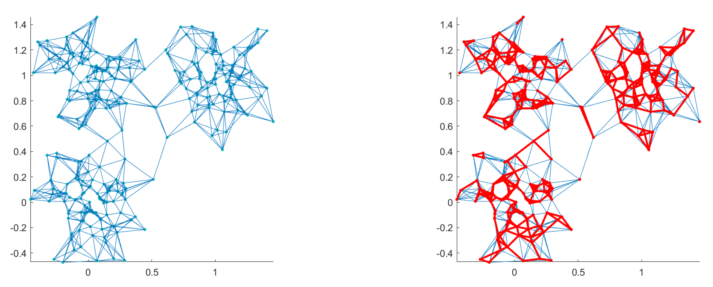
Clustering high dimensional data is a difficult problem in general, and specifically for density-based methods. Here, we seek a solution through KNN graph regularization. The proposed approach, which is applied prior to clustering itself, is taken from [52]. The idea is to optimize the KNN graph, by attempting to preserve only the set of relevant NNs of each sample, and to remove less relevant edges of the graph. Considering an initial directed KNN graph, the approach consists of removing the edges which are not symmetric, so as to transform it into an undirected graph. More precisely, any edge $({\mathbf{x}}_i,{\mathbf{x}}_j)$ of the directed graph $\mathcal{G}$ is retained iff $\left({\mathbf{x}}_i\in {\mathcal{N}}_K\left({\mathbf{x}}_j\right)\right)\wedge \left({\mathbf{x}}_j\in {\mathcal{N}}_K\left({\mathbf{x}}_i\right)\right)$. By doing so, ${\mathbf{x}}_i$ and ${\mathbf{x}}_j$ are nearest neighbors to each other. In this way, the graph does not longer have constant K outdegree: samples which are "popular" nearest neighbors among samples, called hubs [29], have larger outdegrees than samples located on the external borders of clusters. This approach is referred to as the mutual nearest neighbor (MNN) graph modification in the following. Figure 2 illustrates on a simple 2D example (N = 300, 3 clusters) the effect of applying the MNN graph modification on the initial NN graph. In this example, we set $K=11$. One can observe that the set of resulting MNN edges no longer connects the three main data clusters, which makes it easier to identify the latter with density-based methods. However, one drawback of this approach is that it creates small or even single-sample clusters, mainly around the edges of the main clusters.

Concerning implementation, the MNN procedure proceeds by first computing a $N\times N$ sparse binary adjacency matrix from the indices of each sample’s NNs, and computes the logical AND of this matrix with its transpose, thereby retaining only symmetric edges. The result is then recombined into a new NN graph with distance array ${\mathbf{D}}_{MNN}$.

Note that applying MNN naturally associates with each ${\mathbf{x}}_i$ a set of $K_i\le K$ NNs. Several other graph modification methods exist [52,53], but from our experience [54], the MNN graph modification provides better results than the natural nearest neighbor (3N) approach of Zou and Zhu [55].

Once the number $K_i$ of modified neighbors is obtained for each ${\mathbf{x}}_i$ by the MNN procedure, the local density in Equation (2) can be rewritten accordingly as:

$$\begin{array}{c}\hfill \rho \left({\mathbf{x}}_i\right)={\rho }_i=K_i{d}^{-1}({\mathbf{x}}_i,{\mathbf{x}}_{j_i^{K_i}})=K_i{\left({\left[{\mathbf{D}}_{MNN}\right]}_{i,K_i}\right)}^{-1}.\end{array}$$

(4)

We underline that the number of NNs K of the initial graph remains a key parameter of the clustering methods and must be selected carefully.

5.2. Spatial Regularization

In the case of (multi-component) digital images, pixels are considered as samples, and the feature space corresponds to the spectral components. Due to the high correlation between neighboring pixels in images, it can be useful to strengthen their labeling at the local level in the clustering procedure. To achieve this with the four methods described above, we propose to enlarge the set of neighbors of each pixel, by including the set of its spatial neighbors in addition to its NNs in the spectral domain.

Due to the difference in their fundamental principles, the spatial contextualization technique was applied differently to gwenn-wm and m-knnclust-wm on the one hand, and modeseek and m-knn-dpc on the other hand.

Concerning gwenn-wm, let us consider Equation (1), where $Q_i$ is the set of previously processed NNs of the current sample ${\mathbf{x}}_i$ to label. By applying the spatial regularization, $Q_i^{\prime }=P_i\cap ({\mathcal{N}}_K\left({\mathbf{x}}_i\right)\cup \{{\mathbf{x}}_j\in V\left({\mathbf{x}}_i\right)\})$: the intersection of previously processed samples with the union of the current sample’s NNs and the set of its spatial neighbors $V\left({\mathbf{x}}_i\right)$. This rule reinforces the coherence of local labels at little computational expense, provided the spatial context is limited. Concerning m-knnclust-wm, the same scheme can be applied by replacing the set of indices ${\mathbf{j}}_{i_m}$ in the core loop of Algorithm 2 by its union with the spatial neighbors of sample $i_m$.

Concerning m-knn-dpc, the NN search in Equation (3) is modified as follows:

$$\begin{array}{c}\hfill NN\left({\mathbf{x}}_i\right)=arg\underset{j\in ({\mathcal{N}}_K\left({\mathbf{x}}_i\right)\cup \{{\mathbf{x}}_j\in V\left({\mathbf{x}}_i\right)\}):{\rho }_j>{\rho }_i}{min}{d}_{ij}\forall {\mathbf{x}}_i\in \mathcal{X}.\end{array}$$

(5)

The modification is similar for modeseek due to the closeness of the NN search:

$$\begin{array}{c}\hfill NN\left({\mathbf{x}}_i\right)=arg\underset{j\in ({\mathcal{N}}_K\left({\mathbf{x}}_i\right)\cup \{{\mathbf{x}}_j\in V\left({\mathbf{x}}_i\right)\})}{max}{\rho }_j\forall {\mathbf{x}}_i\in \mathcal{X}.\end{array}$$

(6)

In order to account for spatial coherence, we will limit the spatial context to a 4-neighborhood in our experiments for each of the four methods; of course the procedure can easily extend to larger spatial neighborhoods. This issue was not investigated in the present work.

6. Clustering Experiments with the Baseline Methods on Synthetic Datasets

In order to verify the quality of clustering results with the improved baseline methods described in Section 4, we set up a few experiments with synthetic datasets (https://cs.uef.fi/sipu/datasets/). After presenting the clustering performance indices used in the present work, in the first experiment, we wished to assess the improvement of m-knnclust-wm over knnclust-wm. In the second one, we compared the behavior of the four baseline methods on more challenging clustering problems.

6.1. Cluster Validation Indices

All the datasets used in our work include a ground truth, which enables one to compute external classification accuracy indices. Some of these indices are derived from a confusion matrix obtained after optimal pairing of cluster labels with the actual ground truth classes. The cluster-to-class mapping is based on the Munkres assignment algorithm [56]. Once the optimal assignment is obtained, a new confusion matrix is obtained which is close to diagonal. From there, standard classification indices can be derived: the overall accuracy (OA, i.e., the normalized trace of the confusion matrix), the average accuracy (AA, i.e., the average of per-class accuracies) [57] and Cohen’s kappa index of agreement ($\kappa$) [58]. These indices are widely used in the remote sensing community. Other indices are still available, like the adjusted Rand index (ARI) [59], purity and normalized mutual information (NMI) [60] and the centroid similarity index (CSI) [61]. In this work, we also used an internal clustering performance index named the consistency violation ratio (CVR) [62]. The CVR is defined as $\widehat{H}\left(\mathbf{c}\right|\mathcal{X})/\widehat{H}\left(\mathbf{c}\right)$, where the denominator is the entropy of the clustering result $\mathbf{c}$ (obtained with the standard plugin entropy estimate) and the numerator is the entropy of $\mathbf{c}$ conditional on the data observation $\mathcal{X}$. In the present work, the estimate of the latter follows Equation (5) in [62]. By doing this, the computed CVR indices are positive, lower values meaning better clustering.

6.2. Comparison of knnclust Variants

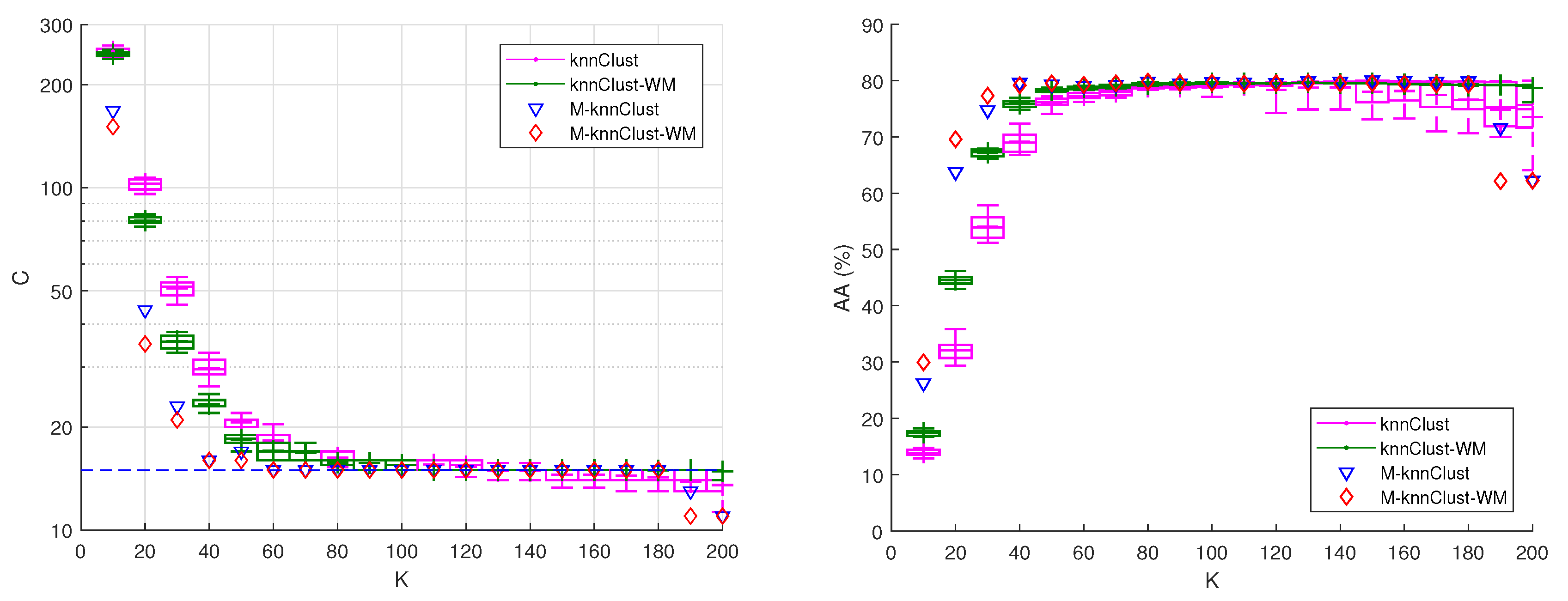
In this experiment, we wished to verify the improvement of m-knnclust-wm over the original knnclust, its weighted mode variant knnclust-wm and m-knnclust, which is the original knnclust algorithm modified according to Section 4.2. The objective was to compare their results in terms of AA as a function of the number of NNs K and to show their ability to provide consistent clustering results, in terms of identification of the correct number of clusters and in clustering accuracy. For this we used the S4 dataset [63] (see Figure 3), which has 5000 samples randomly distributed issued from 15 overlapping Gaussian 2D distributions with various means and covariance matrices. Both features were first normalized in the $[0,1]$ range. Figure 4 reports the number of clusters found as a function of the number of NNs K, and the average accuracy (AA) also versus K. Here, knnclust and knnclust-wm were run 20 times, each time using a different random ordering of the samples, chosen during the initialization stage and kept unchanged during the iterations. Boxplots are displayed on the figures to characterize the distributions of the resulting NC and AA for the latter methods. In contrast, m-knnclust and m-knnclust-wm sort the samples by decreasing local density at the start, so that the results are invariant to the order the samples are processed. Apart from relatively stable results across the clustering results within a large range of NNs K, it was observed that (i) m-knnclust and m-knnclust-wm are able to approach the correct number of clusters with lower K than knnclust and knnclust-wm; (ii) relatedly, m-knnclust and m-knnclust-wm provide higher classification accuracies than knnclust and knnclust-wm on average for low K; (iii) conversely, for higher values of K, m-knnclust and m-knnclust-wm seem to depart from the correct number of clusters faster than the original method on average (for $K>180$). This is due to the fact that a smaller number of clusters was found in this situation. Indeed, primarily accounting for too-distant NNs to label points with high density is likely to result in biased labeling decisions and the merging of samples issued from close clusters in a single larger one. However, since our objective is to achieve the best clustering performances at reduced algorithm complexity, this has no practical relevance. In this sense, the above example seems to indicate that m-knnclust and m-knnclust-wm must be preferred over the original method. Figure 4 also shows the improvement of the weighted mode rule (knnclust-wm and m-knnclust-wm) against the classical mode decision rule (knnclust and m-knnclust). Similar conclusions were obtained after analyzing the S1, S2 and S3 datasets (available on the same website), which are much easier to partition due to smaller overlaps between the generating Gaussian distributions.

6.3. Comparison of the Baseline Clustering Methods

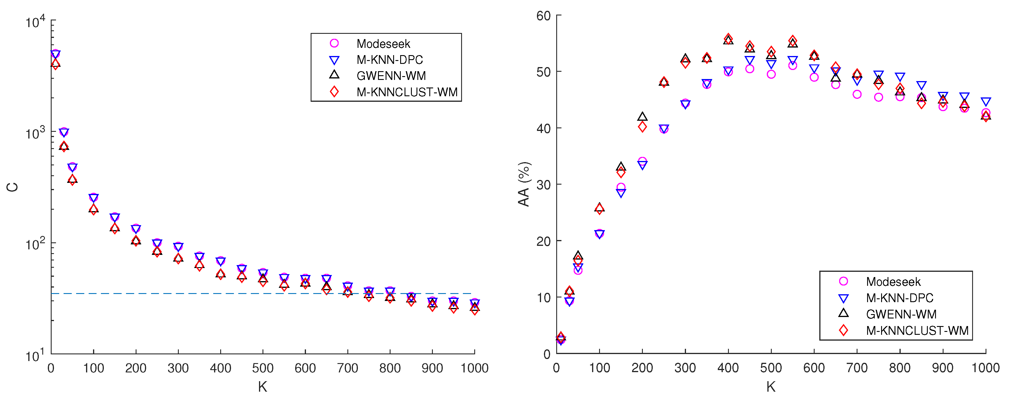
To illustrate the behavior of the four baseline clustering methods described above, we have used the synthetic datasets Worms-2D, with $n=2$, and Worms-64D with $n=64$ [48]. We have selected these datasets because they exhibit curve-shaped clusters with a large amount of overlap or even non-separable data, which represents a very challenging clustering task. Figure 3 displays the Worms-2D dataset, with N = 105,600 points distributed in $C_{\mathrm{true}}=35$ clusters. Figure 5 shows the evolution of the average accuracy (AA) and the number of clusters C as a function of K. The AA values are lower than in the previous example due to the difficulty to cluster this dataset. Still, a tiny plateau of C can be observed for $K\in [550,650]$, giving a number of clusters slightly superior to the actual one. From these figures, one can observe close behaviors between m-knnclust-wm and gwenn-wm on one hand, and between modeseek and m-knn-dpc on the other hand. m-knnclust-wm and gwenn-wm provide a few less clusters than modeseek and m-knn-dpc, thereby yielding higher performance for lower K. For $K>700$, m-knn-dpc provides slightly higher AA values.

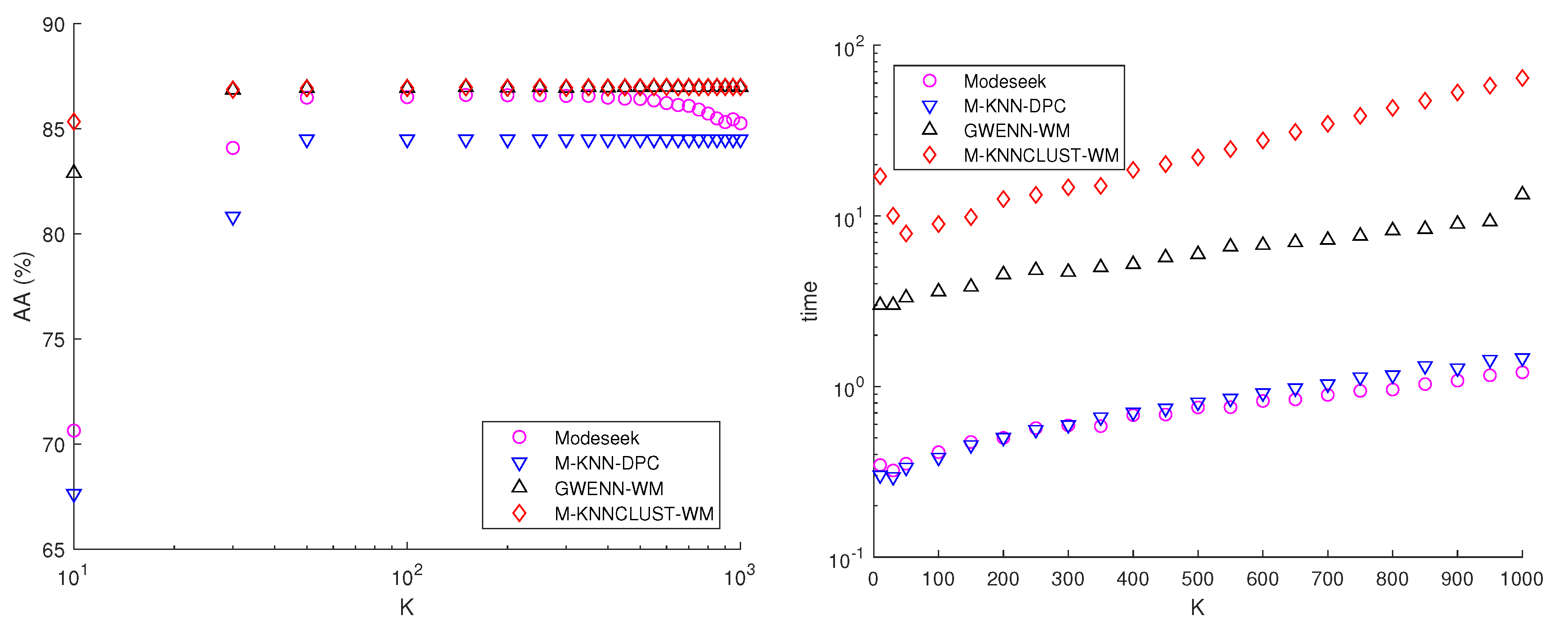
The results for the Worms-64D dataset, shown in Figure 6, show that the AA is stable for a very wide range of K (from 20 to 1000 for m-knnclust-wm and gwenn-wm). Over this range, the correct number of 25 clusters was identified. Here again, m-knnclust-wm and gwenn-wm outperformed the two other methods for all K. It is interesting to notice that modeseek outperformed m-knn-dpc for a large range of K. This illustrates the fact that, for high dimensional data, the choice of the closest NN with higher density can be less relevant than the one of the NN with highest density used in modeseek. Figure 6 also displays the computation times of the four methods as a function of K; the time necessary to compute the KNN graph is not taken into account in this figure. modeseek and m-knn-dpc were the fastest methods, with times increasing linearly with K; in contrast, m-knnclust-wm and gwenn-wm were slower due to the weighted mode procedure, but gwenn-wm was approximately four times faster than m-knnclust-wm.

7. Application to Hyperspectral Remote Sensing Images

In this section, we apply and compare the proposed baseline methods and their HSI-adapted variants to pixel clustering in HSIs. As previously mentioned, this task is challenging due to the high number of pixels to handle and the high dimensionality of data representation. All the HSIs considered here are accompanied with ground truth (GT) maps used for clustering assessment. In the first two experiments, the clustering methods are applied over the whole image support, comprising the pixels which are not labeled in the ground truth. Therefore, the number of final clusters generally exceeds by a few units the actual number of clusters specified in the GT. The section ends up with a study of the clustering results obtained using only the ground truth pixels of three other HSIs.

7.1. AVIRIS—Salinas Hyperspectral Image

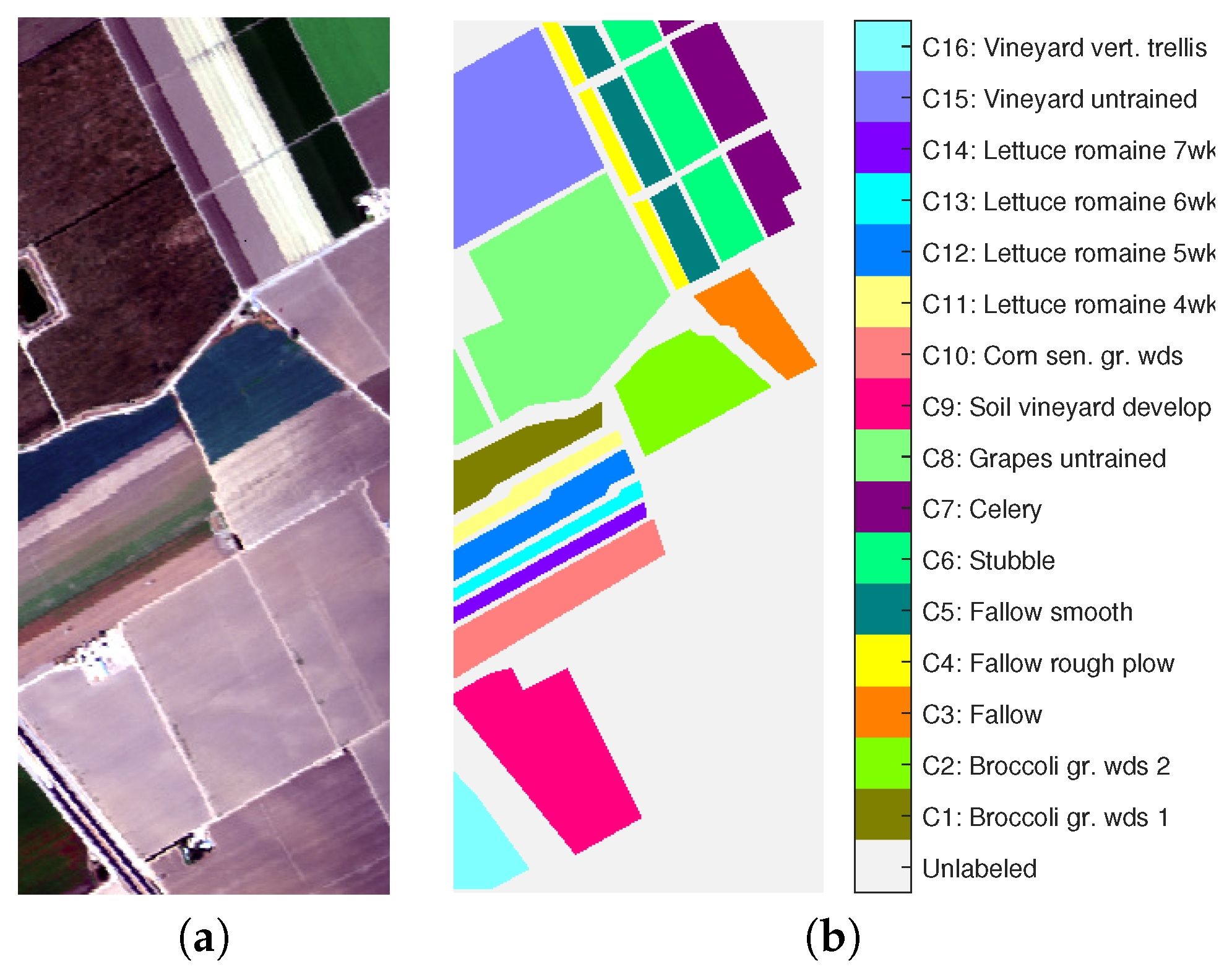
This image (https://www.ehu.eus/ccwintco/index.php/Hyperspectral_Remote_Sensing_Scenes) was acquired by the AVIRIS sensor in 1998 over agricultural fields in the Salinas Valley, California [64]. It has 512 × 217 pixels and 204 spectral bands after absorption and noisy band removal. The ground truth comprises 16 vegetation classes. Figure 7 shows a color composite image, and the associated ground truth. In this experiment, the spectral bands were first individually normalized to zero mean and unit variance before computing KNN graphs based on the Euclidean distance in the representation space ($n=204$). The comparison of the proposed approaches was extended to state-of-the-art methods: fcm, dbscan and a KNN version of the fast sparse affinity propagation method (fsap) proposed by Jia et al. [27]. For dbscan, we empirically sought the values of $MinPts$ and $Eps$ providing the best clustering results. For fcm, the number of output clusters was imposed, the fuzziness parameter was set to 2 and we performed 20 runs of the method with random initial labeling. For fsap, which requires a sequence of two runs of sparse affinity propagation, the preference parameters were selected so as to optimize the external clustering indices.

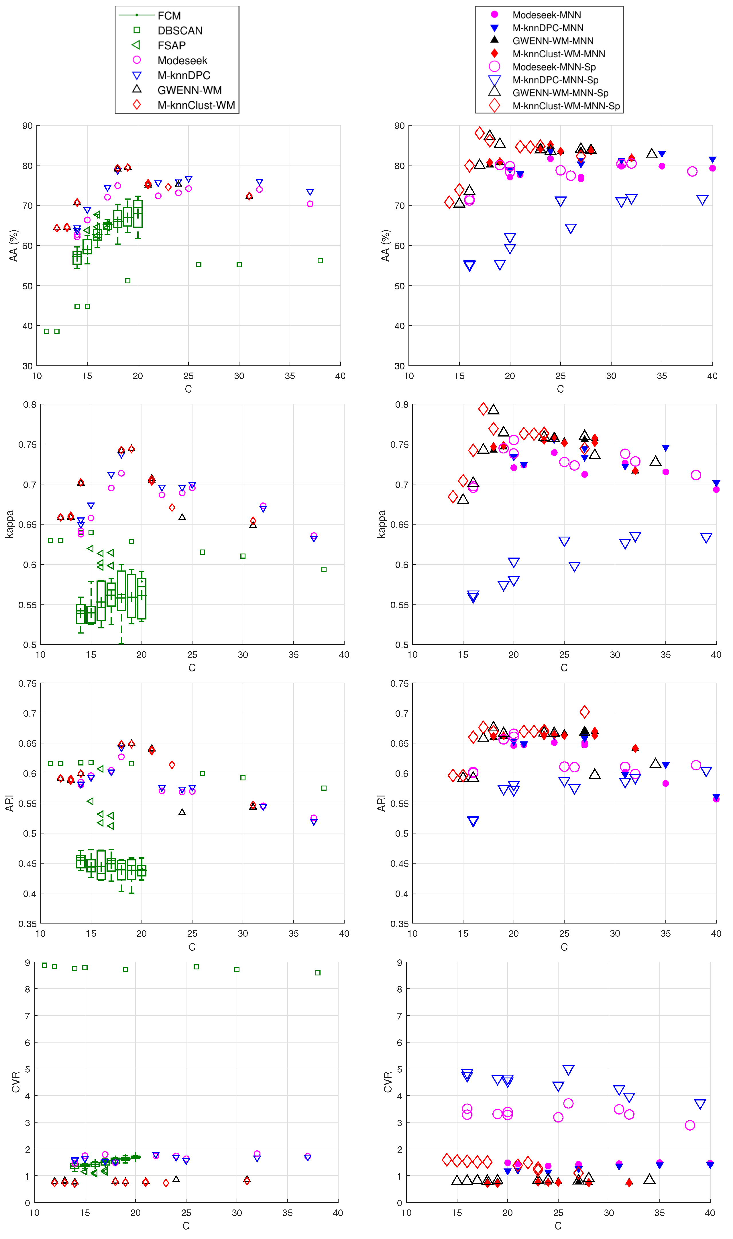
Figure 8 depicts the results of these state-of-the-art methods and the proposed approaches regarding four clustering performance criteria, namely, the AA, the kappa index $\kappa$, the adjusted rand index (ARI) and the CVR index, as functions of the number of clusters provided by the methods. The proposed clustering methods include the set of four baseline methods (modeseek, m-knn-dpc, gwenn-wm, m-knnclust-wm), their respective improvements with the MNN graph regularization (denoted by a -MNN suffix thereafter) and the "spatial" variants of the latter (denoted with a -sp suffix). For each method but fcm (where the free parameter is the number of sought clusters C), K was varied in the range $[300,1200]$ by steps of 100, thereby providing as many clustering results. For fcm, boxplots are plotted for $C\in \{14,\dots ,20\}$ to observe the average and dispersion of the performance indices for the 20 runs of the method. Typically, for all the methods and dbscan and fsap, the number of final clusters decreases with K.

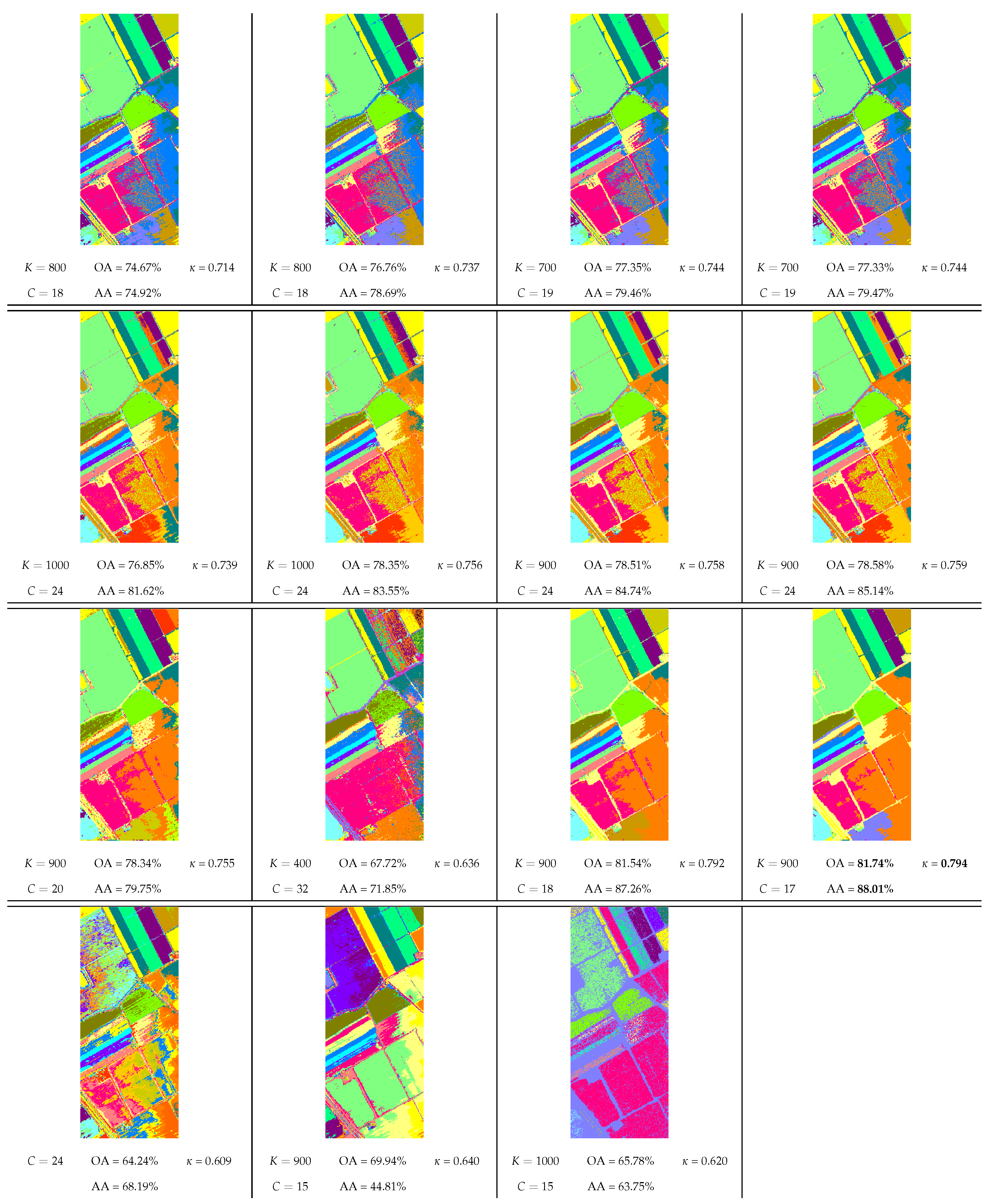
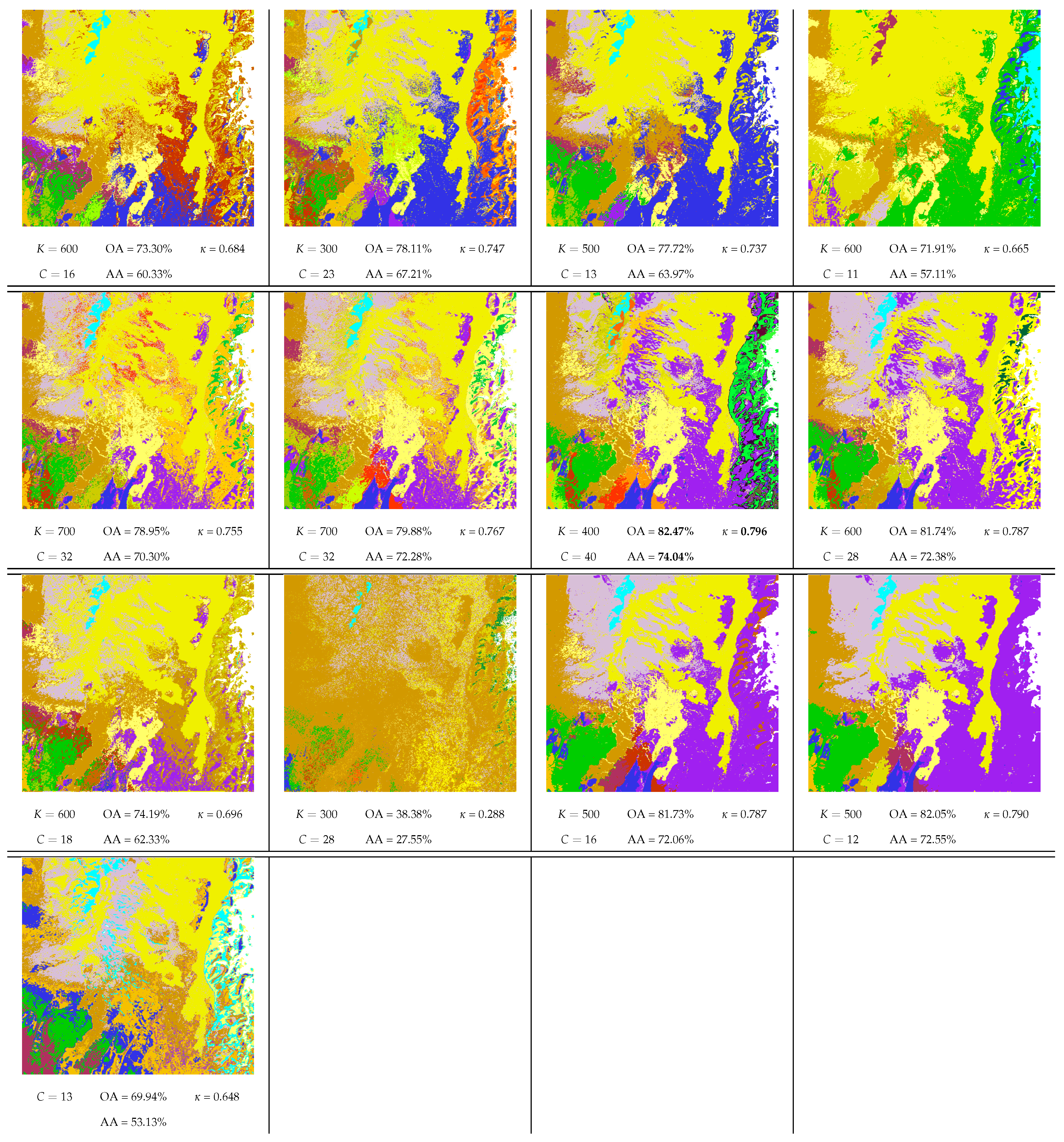
Figure 9 shows the clustering maps obtained from the analysis of this HSI with the baseline density-based methods and their variants, and fcm, fsap and dbscan. For each method, the best clustering result in terms of kappa index is displayed, so that these maps correspond to the highest values of kappa shown in Figure 8. Overall accuracy (OA), average accuracy (AA) and kappa indices are also given for each map.

From this experiment, several observations can be drawn:

• On average, all the nearest-neighbor density-based methods perform better than dbscan, fsap and fcm whatever the number of clusters, found or imposed, and especially regarding the external performance indices. Exceptions to this observation are discussed below.
• Performing MNN graph regularization clearly helps with improving the results for all the methods, but at the cost of creating a higher number of clusters. These are consequences of graph pruning, which tends to create low-density clusters at the border of main clusters, while strengthening the density within the latter, thereby providing more robust results on average.
• The further inclusion of spatial context impacts differently the two subsets of density-based methods, i.e., on the one hand modeseek-mnn and m-knn-dpc-mnn, and on the other hand gwenn-wm-mnn and m-knnclust-mnn. On Figure 8, the performance indices are higher than those without spatial context for the latter subset, and they do not clearly improve or even degrade for the former subset, especially for m-knn-dpc-mnn-sp.
• The best overall kappa index ($\kappa =0.794$) was obtained for m-knnclust-mnn-sp with $K=900$, providing $C=17$ clusters, closely followed by $\kappa =0.792$ for gwenn-wm-mnn-sp with same K, giving $C=18$ clusters. Notice that the running time between those two methods is very different, with 2338 s for m-knnclust-mnn-sp—mostly induced by the high number of labels at initialization—scaling down to 22 s for gwenn-wm-mnn-sp. These times exclude the computation of the original KNN graph, which is about 13 s for $K=1000$ using MATLAB 2016 on a DELL 7810 Precision Tower (20-core, 32GB RAM), and the MNN procedure (78 s).
• The CVR internal clustering indices for the various methods are coherent with the results given by the external indices. It should be mentioned that CVR, contrarily to the other indices, is computed from the extensive cluster map and the original KNN graph, and therefore accounts for all the pixels, should they belong to the GT map or not. The best CVR values are obtained with the subset of gwenn-wm and m-knnclust methods and their MNN and spatial context variants. fcm provides higher CVR values, sometimes better than modeseek and m-knn-dpc.
• Among the state-of-the-art methods used for comparison, fsap provides the best results, at least visually, with a less noisy clustering map. However, there is some amount of confusion between the output clusters and the GT map which lowers the performance indices.
• The classes C8 (grapes untrained) and C15 (vineyard untrained) could not be retrieved by any method. Several published papers already show the difficulty to separate these two classes [65]. However, the class C7 (celery) was split into two clusters with visual coherence by all the density-based methods with MNN graph modification, which confirms the usefulness of this approach for detecting close clusters. This additional cluster disappears with the further use of spatial context which forces the links between those two clusters so as to merge in a single one.
• The only exception regarding the good performances of the proposed methods is with the spatial variant of m-knn-dpc-mnn, which we recall only differs from modeseek by the way the NN of higher local density is selected (see Figure 1). Actually, including spatial neighbors in addition to "spectral" neighbors in this method is likely to drive the NN selection to the spectrally closest spatial neighbors, thereby separating compact clusters into subclusters while achieving the same final number of clusters as modeseek, as said above, hence dramatically reducing the clustering performance. In comparison, the NN selection rule set up in modeseek is more robust to some extent.

7.2. AVIRIS—Hekla Hyperspectral Image

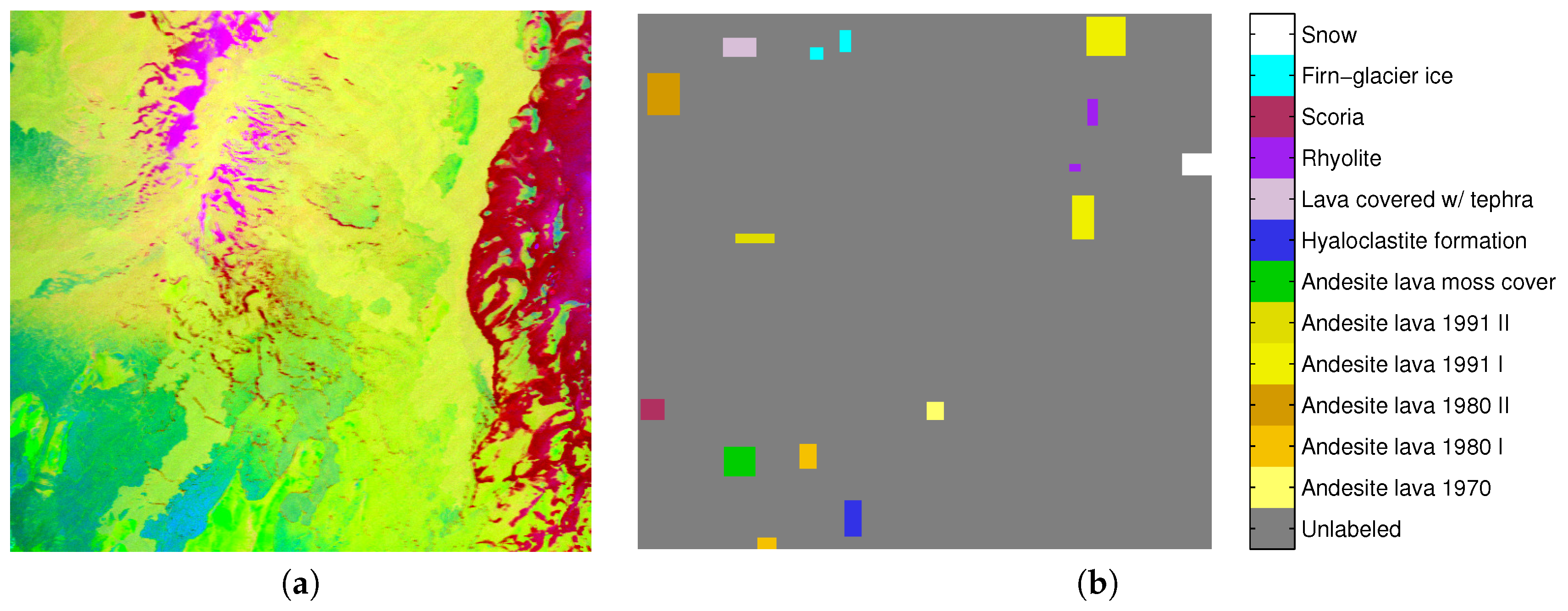
This HSI was acquired in 1991 by AVIRIS over the Hekla volcano in Iceland. The image has $560\times 600$ pixels (approximately thrice the number of pixels of the previous image) and 157 spectral bands [66]. Here, the original image was preprocessed with the minimum noise fraction algorithm (MNF) [67], and 10 principal components were retained for clustering. Figure 10 shows a color image of the first three MNF components, and the ground truth used for assessment and comprising 12 land-cover classes. The KNN graphs were computed for K in the range $[400,2000]$ by steps of 100, and the proposed methods were applied and compared similarly as in the above example. For this image, it was not possible to find appropriate parameters to run dbscan and fsap, and only fcm results were computed for $C\in \{10,\dots ,30\}$. Figure 11 shows the corresponding performance results. Though the data preprocessing stage was different from the previous example, the conclusions drawn from these results remained the same and confirmed the superiority of the nearest-neighbor density-based methods with respect to fcm. The improvement brought by both symmetrizing the initial KNN graph and introducing the spatial context in the density-based methods is also significant with this HSI, except again for m-knn-dpc-mnn-sp, and modeseek-mnn-sp to a lower extent. Again, adding the spatial context after MNN significantly reduces the number of clusters. The best overall clustering result with regard to the kappa index is obtained by gwenn-wm-mnn with ($\kappa$ = 0.796 for $K=400$), with a high number of clusters ($C=40$) found. The following best ones are provided both for $K=500$ by m-knnclust-mnn-sp ($\kappa$ = 0.7905, $C=12$) and gwenn-wm-mnn-sp ($\kappa$ = 0.7868, $C=16$). Additionally, similar trends as with the previous HSI regarding the ARI and CVR indices were obtained.

Figure 12 shows the clustering maps corresponding to the best results in terms of kappa index for the four proposed methods and their variants, along with the best fcm result. Again, the spatial coherence of the clustering maps is reinforced for gwenn-wm-mnn-sp and m-knnclust-mnn-sp with respect to their non-spatial counterparts. Contrarily, m-knn-dpc-mnn-sp totally fails in retrieving the correct clusters, with a main cluster covering approximately 2/3 of the clustering map. In comparison, modeseek-mnn-sp performs better, like with the Salinas HSI.

7.3. Other Hyperspectral Images

A last experiment was set up with a set of three other HSIs:

• The DC Mall HSI (https://engineering.purdue.edu/~biehl/MultiSpec/hyperspectral.html) (1280 × 307 pixels, 191 spectral bands), acquired in 1995 over Washington, DC by the HYDICE instrument; the corresponding ground truth has 43368 pixels distributed in seven thematic classes [68];
• The Kennedy Space Center (KSC) HSI (https://www.ehu.es/ccwintco/index.php/Hyperspectral_Remote_Sensing_Scenes) (614 × 512 pixels, 176 spectral bands), acquired in 1996 over Titusville, Florida, by the AVIRIS sensor; the ground truth has 5211 pixels in 13 classes [53];
• The Massey University HSI (1579 × 1618 pixels, 339 spectral bands), acquired over Palmerston North, New Zealand, by the AisaFENIX sensor (Specim Ltd., Finland); the ground truth has 9564 pixels in 23 classes [53].

In this experiment, clustering was applied exclusively on the labeled pixels of the GT map. By doing so, it was not possible to apply the spatial context versions of the nearest-neighbor density-based methods, so we limited the study to the original methods and their MNN versions. Therefore, the KNN graphs were calculated from those labeled pixels. fcm (with varying C) and dbscan (with optimized parameters) were also used for comparison. No prior data normalization was applied the three HSIs.

Table 3. Comparison of several clustering performance indices and numbers of clusters found for various HSIs and different clustering methods. For each method, these results correspond to the best kappa index obtained as a function of K.

Optimal K, #Clusters and Criteria →		K	C	AA	OA	$\mathit{\kappa }$	Purity	NMI	CVR
DC Mall : N = 43,368, $n=191$, $C_{true}$ = 7
	modeseek	2200	5	61.72	82.22	0.777	0.874	0.721	1.431
Constant	m-knn-dpc	2200	5	63.57	84.43	0.805	0.898	0.753	0.874
K	gwenn-wm	3000	5	62.53	82.97	0.787	0.883	0.743	0.716
	m-knnclust-wm	3000	5	62.96	83.63	0.795	0.890	0.745	0.706
MNN	modeseek-mnn	3000	6	73.07	84.45	0.809	0.873	0.756	0.654
	m-knn-dpc-mnn	3000	6	72.86	84.35	0.808	0.872	0.756	0.657
	gwenn-wm-mnn	3000	6	73.05	84.81	0.813	0.877	0.762	0.521
	m-knnclust-wm-mnn	3000	6	73.04	84.82	0.813	0.877	0.763	0.521
fcm		-	6	71.06	80.01	0.754	0.827	0.717	1.179
dbscan		320	5	37.86	76.63	0.608	0.778	0.591	2.116
KSC : N = 5211, $n=176$, $C_{true}$ = 13
	modeseek	120	9	42.44	52.58	0.478	0.685	0.592	1.807
Constant	m-knn-dpc	120	9	45.18	57.15	0.526	0.730	0.641	1.373
K	gwenn-wm	110	9	44.15	56.75	0.521	0.730	0.633	0.731
	m-knnclust-wm	110	9	44.26	56.88	0.523	0.730	0.634	0.713
MNN	modeseek-mnn	150	10	43.92	57.59	0.531	0.718	0.628	2.794
	m-knn-dpc-mnn	150	10	46.54	60.45	0.563	0.751	0.672	2.241
	gwenn-wm-mnn	140	9	43.86	57.34	0.526	0.752	0.646	1.617
	m-knnclust-wm-mnn	130	9	44.04	57.49	0.528	0.752	0.647	1.337
fcm		-	11	40.60	52.29	0.471	0.604	0.560	5.383
dbscan		70	9	47.68	68.23	0.530	0.692	0.795	104.0
Massey University : N = 9564, $n=339$, $C_{true}$ = 23
	modeseek	130	14	38.33	51.49	0.460	0.725	0.625	2.860
Constant	m-knn-dpc	130	14	39.19	53.32	0.479	0.746	0.672	2.060
K	gwenn-wm	110	16	41.09	52.97	0.480	0.702	0.664	0.990
	m-knnclust-wm	110	16	41.08	52.89	0.480	0.703	0.668	0.949
MNN	modeseek-mnn	130	22	45.29	55.73	0.507	0.715	0.669	2.380
	m-knn-dpc-mnn	130	22	50.72	60.78	0.564	0.747	0.729	1.639
	gwenn-wm-mnn	110	27	55.39	59.06	0.552	0.684	0.738	0.961
	m-knnclust-wm-mnn	110	28	55.27	57.69	0.544	0.621	0.727	1.073
fcm		-	21	39.41	40.73	0.371	0.471	0.603	8.859
dbscan		450	4	6.28	75.07	0.589	0.751	0.753	87.11

shows the results corresponding to the highest kappa values obtained with the various approaches after varying K within a large range, specific to each HSI. Several performance indices are reported, namely, AA, OA, $\kappa$, purity, NMI and CVR. The latter three are useful to assess the consistency of the results; indeed, high values of OA, AA or kappa after cluster assignment are not sufficient to measure high quality clustering, especially in the case where the number of GT classes is greater than the number of found clusters.

Again, the nearest-neighbor density-based methods show superior performance to the popular fcm in all cases. The situation is less clear for dbscan which seems to provide better accuracy indices for the KSC and Massey University HSIs. Actually, for the KSC dataset, the clustering results for dbscan were calculated only over 25% of the number of pixels (so-called “core points”), the remainder being classified as outliers by dbscan. For the Massey University HSI, the number of outliers provided by dbscan exceeded 96% of the number of pixels. Thus, the best OA results provided by dbscan must be considered with caution. However, the high CVR indices given by dbscan for these two HSIs can help with detecting this kind of anomalous situation.

Many of these best kappa results come with an underestimation by a few units of the actual number of classes present in the GT. However, on average the number of clusters is better approximated by applying the MNN graph regularization prior to density-based clustering. This was particularly observed for the Massey University HSI which has roughly twice the dimensionality of the other ones.

To some extent, these results on various hyperspectral datasets are in agreement with the preceding observations made in the above experiments, as shown by the good performances of the proposed approaches versus state-of-the-art clustering methods, and the improvement brought by the MNN graph pruning procedure.

8. Conclusions

In this paper, we have proposed several improvements to existing nearest-neighbor density-based clustering methods, and considered their application to pixel clustering in hyperspectral images. These methods use a KNN graph to estimate local (point-wise) density values which are then used to propagate labeling decisions specific to each method.

Our contributions are twofold. First, we improved two of these methods, namely, knnclust-wm and a KNN variant of dpc. The former method was modified to account for the local density as prior information to foster the labeling decisions corresponding to samples by decreasing order of their density. The latter one was completely revisited to avoid the use of a decision graph and threshold, and we showed that the resulting algorithm is very close to modeseek. Second, we proposed using two additional procedures to help with tackling the problem of pixel partitioning in hyperspectral images. The first relies on a KNN graph pruning method based on mutual nearest neighbors (MNN), which can facilitate the discovery of clusters in high dimensional datasets. This procedure is applied prior to the baseline clustering methods. The second one aims to introduce a spatial context in the core of each clustering method, in order to account for the correlation between adjacent pixels in hyperspectral images.

The improved knnclust-wm method and the set of baseline nearest-neighbor density-based methods modeseek, m-knn-dpc, gwenn-wm and m-knnclust-wm were then tested and compared on synthetic datasets, showing their ability to adequately cluster points issued from highly overlapping conditional densities in low and high dimensions. The enhanced methods, using the MNN, and then combining MNN and spatial context, were then applied to a benchmark of real hyperspectral images, and compared with state-of-the-art methods, namely, fcm, dbscan and fsap. The experimental results show that the proposed improvements of the baseline nearest-neighbor density-based methods increase the clustering performance in most cases in terms of standard classification accuracy and other clustering indices. In particular, the graph and spatial improvements of gwenn and knnclust provide the best results on average, outperforming the state-of-the-art methods by more than 20% in optimal kappa index for varying K on real hyperspectral images; while the results of these methods are close to each other, gwenn is much faster than knnclust due to its non-iterative feature. Additionally, m-knn-dpc generally performs better than modeseek in the baseline and MNN improved versions; this is, however, no longer true for their spatial versions, due to the difference pointed out between their respective core labeling rules, and modeseek should then be preferred to m-knn-dpc. From a more general viewpoint, unlike other methods like dbscan and fsap which are sensitive to parameter tuning, the proposed approaches require only one parameter, i.e., the number of nearest neighbors K.

In conclusion, owing to their attractive features, the nearest-neighbor density-based methods investigated in this paper do constitute a viable alternative to traditional clustering methods in the context of hyperspectral images: they are able to closely predict the number of clusters present in a dataset with minimal parametrization; they are strictly deterministic and therefore do not rely on a random initialization stage.

Although only HSIs were considered here, nearest-neighbor density-based methods can also be applied to other remote sensing image data, such as very high resolution multispectral images. To this end, the proposed improvements can be implemented in a multi-resolution framework, following [32,40].

However, many issues still remain, the most important of which is the automatic tuning of K. The choices of the best distance metrics among high-dimensional samples and the best local density model are also critical design choices. These aspects are currently under investigation.

References

1. Min, E.; Guo, X.; Liu, Q.; Zhang, G.; Cui, J.; Long, J. A Survey of Clustering With Deep Learning: From the Perspective of Network Architecture. IEEE Access 2018, 6, 39501–39514. [Google Scholar] [CrossRef]
2. MacQueen, J.B. Some Methods for Classification and Analysis of MultiVariate Observations. In Proceedings of the Fifth Berkeley Symposium on Mathematical Statistics and Probability; University of California Press: Berkeley, CA, USA, 1967; Volume 1, pp. 281–297. [Google Scholar]
3. Bezdek, J. Pattern Recognition With Fuzzy Objective Function Algorithms; Plenum Press: New York, NY, USA, 1981. [Google Scholar]
4. Ward, J. Hierarchical grouping to optimize an objective function. J. Am. Stat. Assoc. 1963, 58, 236–244. [Google Scholar] [CrossRef]
5. Sneath, P.; Sokal, R. Numerical Taxonomy. The Principles and Practice of Numerical Classification; Freeman: London, UK, 1973. [Google Scholar]
6. Ester, M.; Kriegel, H.P.; Sander, J.; Xu, X. A Density-Based Algorithm for Discovering Clusters in Large Spatial Databases with Noise. In Proceedings of the Second International Conference on Knowledge Discovery and Data Mining (KDD’96), Portland, OR, USA, 2–4 August 1996; pp. 226–231. [Google Scholar]
7. Ankerst, M.; Breunig, M.M.; Kriegel, H.P.; Sander, J. OPTICS: Ordering Points To Identify the Clustering Structure. In Proceedings of the ACM SIGMOD International Conference on Management of Data (SIGMOD’99), Philadelphia, PA, USA, 31 May–3 June 1999; pp. 49–60. [Google Scholar]
8. Fukunaga, K.; Hostetler, L.D. The estimation of the gradient of a density function, with applications in pattern recognition. IEEE Trans. Inf. Theory 1975, 21, 32–40. [Google Scholar] [CrossRef] [Green Version]
9. Koontz, W.L.G.; Narendra, P.M.; Fukunaga, K. A Graph-Theoretic Approach to Nonparametric Cluster Analysis. IEEE Trans. Comput. 1976, 25, 936–944. [Google Scholar] [CrossRef]
10. Duin, R.P.W.; Fred, A.L.N.; Loog, M.; Pekalska, E. Mode Seeking Clustering by KNN and Mean Shift Evaluated. In Proceedings of the SSPR/SPR, Hiroshima, Japan, 7–9 November 2012; Lecture Notes in Computer Science. Springer: Berlin/Heidelberg, Germany, 2012; Volume 7626, pp. 51–59. [Google Scholar]
11. Rodriguez, A.; Laio, A. Clustering by fast search and find of density peaks. Science 2014, 344, 1492–1496. [Google Scholar] [CrossRef] [PubMed] [Green Version]
12. Dempster, A.P.; Laird, N.M.; Rubin, D.B. Maximum likelihood from incomplete data via the EM algorithm. J. R. Stat. Soc. Series B. 1977, 39, 1–38. [Google Scholar]
13. Celeux, G.; Govaert, G. A classification EM algorithm for clustering and two stochastic versions. Comput. Stat. Data Anal. 1992, 14, 315–332. [Google Scholar] [CrossRef] [Green Version]
14. Rasmussen, C.E. The Infinite Gaussian Mixture Model. In Proceedings of the 12th International Conference on Neural Information Processing Systems (NIPS’99), 29 November–4 Decemeber 1999; Solla, S.A., Leen, T.K., Müller, K.R., Eds.; MIT Press: Cambridge, MA, USA, 2000; pp. 554–560. [Google Scholar]
15. Shi, J.; Malik, J. Normalized Cuts and Image Segmentation. IEEE Trans. Pattern Anal. Mach. Intell. 2000, 22, 888–905. [Google Scholar]
16. Schölkopf, B.; Smola, A.; Müller, K.R. Nonlinear component analysis as a kernel eigenvalue problem. Neural Comput. 1998, 10, 1299–1319. [Google Scholar] [CrossRef] [Green Version]
17. Frey, B.J.; Dueck, D. Clustering by Passing Messages Between Data Points. Science 2007, 315, 972–976. [Google Scholar] [CrossRef] [Green Version]
18. Sugiyama, M.; Niu, G.; Yamada, M.; Kimura, M.; Hachiya, H. Information-Maximization Clustering Based on Squared-Loss Mutual Information. Neural Comput. 2014, 26, 84–131. [Google Scholar] [CrossRef] [PubMed]
19. Hocking, T.; Vert, J.P.; Bach, F.R.; Joulin, A. Clusterpath: An Algorithm for Clustering using Convex Fusion Penalties. In Proceedings of the 28th International Conference on International Conference on Machine Learning (ICML’11), Bellevue, WA, USA, 28 June–2 July 2011; pp. 745–752. [Google Scholar]
20. Elhamifar, E.; Vidal, R. Sparse Subspace Clustering: Algorithm, Theory, and Applications. IEEE Trans. Pattern Anal. Mach. Intell. 2013, 35, 2765–2781. [Google Scholar] [CrossRef] [PubMed] [Green Version]
21. Chazal, F.; Guibas, L.J.; Oudot, S.Y.; Skraba, P. Persistence-Based Clustering in Riemannian Manifolds. J. ACM 2013, 60, 38. [Google Scholar] [CrossRef]
22. Masulli, F.; Rovetta, S. Clustering High-Dimensional Data. In Proceedings of the 1st International Workshop on Clustering High-Dimensional Data (Revised Selected Papers); Volume LNCS-7627, New York, NY, USA, 2015; Volume Springer, pp. 1–13. [Google Scholar]
23. Xu, R.; Wunsch, D. Survey of clustering algorithms. IEEE Trans. Neural Netw. 2005, 16, 645–678. [Google Scholar] [CrossRef] [PubMed] [Green Version]
24. Tran, T.N.; Wehrens, R.; Buydens, L.M.C. KNN-kernel density-based clustering for high-dimensional multivariate data. Comput. Stat. Data Anal. 2006, 51, 513–525. [Google Scholar] [CrossRef]
25. Cariou, C.; Chehdi, K. Unsupervised Nearest Neighbors Clustering with Application to Hyperspectral Images. IEEE J. Sel. Top. Signal Process. 2015, 9, 1105–1116. [Google Scholar] [CrossRef] [Green Version]
26. Xie, J.; Gao, H.; Xie, W.; Liu, X.; Grant, P.W. Robust clustering by detecting density peaks and assigning points based on fuzzy weighted K-nearest neighbors. Inf. Sci. 2016, 354, 19–40. [Google Scholar] [CrossRef]
27. Jia, Y.; Wang, J.; Zhang, C.; Hua, X.S. Finding image exemplars using fast sparse affinity propagation. In ACM Multimedia; El-Saddik, A., Vuong, S., Griwodz, C., Bimbo, A.D., Candan, K.S., Jaimes, A., Eds.; ACM: New York, NY, USA, 2008; pp. 639–642. [Google Scholar]
28. Hinneburg, A.; Aggarwal, C.C.; Keim, D.A. What Is the Nearest Neighbor in High Dimensional Spaces? In Proceedings of the 26th VLDB Conference, Cairo, Egypt, 10–14 September 2000; Abbadi, A.E., Brodie, M.L., Chakravarthy, S., Dayal, U., Kamel, N., Schlageter, G., Whang, K.Y., Eds.; Morgan Kaufmann: San Fransisco, CA, USA, 2000; pp. 506–515. [Google Scholar]
29. Radovanovic, M.; Nanopoulos, A.; Ivanovic, M. Hubs in Space: Popular Nearest Neighbors in High-Dimensional Data. J. Mach. Learn. Res. 2010, 11, 2487–2531. [Google Scholar]
30. Arya, S.; Mount, D.; Netanyahu, N.; Silverman, R.; Wu, A. An Optimal Algorithm for Approximate Nearest Neighbor Searching Fixed Dimensions. J. ACM 1998, 45, 891–923. [Google Scholar] [CrossRef] [Green Version]
31. Fränti, P.; Virmajoki, O.; Hautamäki, V. Fast Agglomerative Clustering Using a k-Nearest Neighbor Graph. IEEE Trans. Pattern Anal. Mach. Intell. 2006, 28, 1875–1881. [Google Scholar] [CrossRef]
32. Cariou, C.; Chehdi, K. A new k-nearest neighbor density-based clustering method and its application to hyperspectral images. In Proceedings of the IEEE International Geoscience and Remote Sensing Symposium, Beijing, China, 10–15 July 2016; pp. 6161–6164. [Google Scholar]
33. Goodenough, D.G.; Chen, H.; Richardson, A.; Cloude, S.; Hong, W.; Li, Y. Mapping fire scars using Radarsat-2 polarimetric SAR data. Can. J. Remote Sens. 2011, 37, 500–509. [Google Scholar] [CrossRef] [Green Version]
34. Du, M.; Ding, S.; Jia, H. Study on density peaks clustering based on k-nearest neighbors and principal component analysis. Knowl.-Based Syst. 2016, 99, 135–145. [Google Scholar] [CrossRef]
35. Yaohui, L.; Ma, Z.; Fang, Y. Adaptive density peak clustering based on K-nearest neighbors with aggregating strategy. Knowl.-Based Syst. 2017, 133, 208–220. [Google Scholar] [CrossRef]
36. Wang, G.; Song, Q. Automatic Clustering via Outward Statistical Testing on Density Metrics. IEEE Trans. Knowl. Data Eng. 2016, 28, 1971–1985. [Google Scholar] [CrossRef]
37. Liu, R.; Wang, H.; Yu, X. Shared-nearest-neighbor-based clustering by fast search and find of density peaks. Inf. Sci. 2018, 450, 200–226. [Google Scholar] [CrossRef]
38. Vincent, L.; Soille, P. Watersheds in Digital Spaces: An Efficient Algorithm Based on Immersion Simulations. IEEE Trans. PAMI 1991, 13, 583–598. [Google Scholar] [CrossRef] [Green Version]
39. Desquesnes, X.; Elmoataz, A.; Lézoray, O. Eikonal Equation Adaptation on Weighted Graphs: Fast Geometric Diffusion Process for Local and Non-local Image and Data Processing. J. Math. Imaging Vis. 2013, 46, 238–257. [Google Scholar] [CrossRef] [Green Version]
40. Cariou, C.; Chehdi, K. Nearest-neighbor density-based clustering methods for large hyperspectral images. In Proceedings of the SPIE Image and Signal Processing for Remote Sensing XXIII, Warsaw, Poland, 11–14 September 2017; Volume 10427. [Google Scholar] [CrossRef] [Green Version]
41. Cariou, C.; Chehdi, K. Application of unsupervised nearest-neighbor density-based approaches to sequential dimensionality reduction and clustering of hyperspectral images. In Proceedings of the SPIE Image and Signal Processing for Remote Sensing XXIV, Berlin, Germany, 10–13 September 2018; Volume 10789. [Google Scholar]
42. Aggarwal, C.C.; Hinneburg, A.; Keim, D.A. On the surprising behavior of distance metrics in high dimensional space. In Lecture Notes in Computer Science; Springer: Berlin, Germany, 2001; pp. 420–434. [Google Scholar]
43. Mahalanobis, P.C. On the generalized distance in statistics. Proc. Natl. Inst. Sci. (Calcutta) 1936, 2, 49–55. [Google Scholar]
44. Xu, X.; Ju, Y.; Liang, Y.; He, P. Manifold Density Peaks Clustering Algorithm. In Proceedings of the Third International Conference on Advanced Cloud and Big Data, Yangzhou, China, 30 October–1 November 2015; IEEE Computer Society: Piscataway, NJ, USA, 2015; pp. 311–318. [Google Scholar] [CrossRef]
45. Du, M.; Ding, S.; Xu, X.; Xue, Y. Density peaks clustering using geodesic distances. Int. J. Mach. Learn. Cybern. 2018, 9, 1335–1349. [Google Scholar] [CrossRef]
46. Schölkopf, B. The Kernel Trick for Distances. In Proceedings of the 13th International Conference on Neural Information Processing Systems (NIPS’00); Leen, T.K., Dietterich, T.G., Tresp, V., Eds.; MIT Press: Cambridge, MA, USA, 2000; pp. 283–289. [Google Scholar]
47. Scott, D.W.; Sain, S.R. Multi-dimensional density estimation. In Data Mining and Data Visualization; Handbook of Statistics: Amsterdam, The Netherlands, 2005; Volume 24. [Google Scholar]
48. Sieranoja, S.; Fränti, P. Fast and general density peaks clustering. Pattern Recognit. Lett. 2019, 128, 551–558. [Google Scholar] [CrossRef]
49. Geng, Y.A.; Li, Q.; Zheng, R.; Zhuang, F.; He, R.; Xiong, N. RECOME: A new density-based clustering algorithm using relative KNN kernel density. Inf. Sci. 2018, 436–437, 13–30. [Google Scholar] [CrossRef] [Green Version]
50. Le Moan, S.; Cariou, C. Parameter-Free Density Estimation for Hyperspectral Image Clustering. In Proceedings of the International Conference on Image and Vision Computing New Zealand (IVCNZ), Auckland, New Zealand, 19–21 November 2018. [Google Scholar]
51. Liang, Z.; Chen, P. Delta-density based clustering with a divide-and-conquer strategy: 3DC clustering. Pattern Recognit. Lett. 2016, 73, 52–59. [Google Scholar] [CrossRef]
52. Stevens, J.R.; Resmini, R.G.; Messinger, D.W. Spectral-Density-Based Graph Construction Techniques for Hyperspectral Image Analysis. IEEE Trans. Geosci. Remote Sens. 2017, 55, 5966–5983. [Google Scholar] [CrossRef]
53. Le Moan, S.; Cariou, C. Minimax Bridgeness-Based Clustering for Hyperspectral Data. Remote Sens. 2020, 12, 1162. [Google Scholar] [CrossRef] [Green Version]
54. Cariou, C.; Chehdi, K.; Le Moan, S. Improved Nearest Neighbor Density-Based Clustering Techniques with Application to Hyperspectral Images. In Proceedings of the IEEE International Conference on Acoustics, Speech and Signal Processing (ICASSP), Barcelona, Spain, 4–8 May 2020; pp. 4127–4131. [Google Scholar]
55. Zou, X.; Zhu, Q. Adaptive Neighborhood Graph for LTSA Learning Algorithm without Free-Parameter. Int. J. Comput. Appl. 2011, 19, 28–33. [Google Scholar]
56. Kuhn, H. The Hungarian method for the assignment problem. Nav. Res. Logist. Q. 1955, 2, 83–97. [Google Scholar] [CrossRef] [Green Version]
57. Tarabalka, Y.; Benediktsson, J.A.; Chanussot, J. Spectral-spatial classification of hyperspectral imagery based on partitional clustering techniques. IEEE Trans. Geosci. Remote Sens. 2009, 47, 2973–2987. [Google Scholar] [CrossRef]
58. Cohen, J. A coefficient of agreement for nominal scales. Educ. Psychol. Meas. 1960, 20, 37–46. [Google Scholar] [CrossRef]
59. Hubert, L.; Arabie, P. Comparing partitions. J. Classif. 1985, 2, 193–218. [Google Scholar] [CrossRef]
60. Manning, C.D.; Raghavan, P.; Schütze, H. An Introduction to Information Retrieval; Cambridge University Press: Cambridge, UK, 2008. [Google Scholar]
61. Fränti, P.; Rezaei, M.; Zhao, Q. Centroid index: Cluster level similarity measure. Pattern Recognit. 2014, 47, 3034–3045. [Google Scholar] [CrossRef]
62. Ver Steeg, G.; Galstyan, A.; Sha, F.; DeDeo, S. Demystifying Information-Theoretic Clustering. In Proceedings of the 31st International Conference on Machine Learning, Beijing, China, 22–24 June 2014. [Google Scholar]
63. Fränti, P.; Sieranoja, S. How much can k-means be improved by using better initialization and repeats? Pattern Recognit. 2019, 93, 95–112. [Google Scholar] [CrossRef]
64. Gualtieri, J.A.; Chettri, S.R.; Cromp, R.F.; Johnson, L.F. Support Vector Machine Classifiers as Applied to AVIRIS Data. In Proceedings of the Summaries of the Eighth JPL Airborne Earth Science Workshop, Pasadena, CA, USA, 9–11 February 1999; JPL-NASA: Pasadena, CA, USA, 1999; pp. 1–10. [Google Scholar]
65. Huang, S.; Zhang, H.; Du, Q.; Pizurica, A. Sketch-Based Subspace Clustering of Hyperspectral Images. Remote Sens. 2020, 12, 775. [Google Scholar] [CrossRef] [Green Version]
66. Waske, B.; Benediktsson, J.A.; Árnason, K.; Sveinsson, J.R. Mapping of hyperspectral AVIRIS data using machine-learning algorithms. Can. J. Remote Sens. 2009, 35, S106–S116. [Google Scholar] [CrossRef]
67. Green, A.A.; Berman, M.; Switzer, P.; Graig, M.D. A transformation for ordering multispectral data in terms of image quality with implications for noise removal. IEEE Trans. Geosci. Remote Sens. 1988, 26, 65–74. [Google Scholar] [CrossRef] [Green Version]
68. Landgrebe, D. Hyperspectral image data analysis. IEEE Signal Process. Mag. 2002, 19, 17–28. [Google Scholar] [CrossRef]
Figure 1. Illustration of the difference between the neighbor search strategies of modeseek and m-knn-dpc. modeseek retains, among the current sample x i and its K nearest neighbors, the one with the highest density (here the fourth NN), whereas m-knn-dpc retains the closest with higher density than the current sample (here the second NN).
Remotesensing 12 03745 g001
Figure 2. Illustration of the MNN graph modification on a 2D dataset with K = 11 . Left: data samples and edges of initial graph; right: resulting MNN edges (red lines).
Remotesensing 12 03745 g002
Figure 3. The S4 (left) and Worms_2d (right) datasets. Each color represents a specific cluster.
Remotesensing 12 03745 g003
Figure 4. Comparison of knnclust (black circles, 10 runs), m-knnclust (blue triangles) and m-knnclust-wm (red stars) as functions of the number of NNs K on the S4 dataset. Left: Number of clusters C found (true number of clusters as a dotted line); right: average accuracy.
Remotesensing 12 03745 g004
Figure 5. Comparison of the four baseline methods as a function of the number of NNs K on the Worms-2D dataset. Left: Number of found clusters C (true number of clusters in dotted line); right: average accuracy.
Remotesensing 12 03745 g005
Figure 6. Comparison of the four baseline methods as a function of the number of NNs K on the Worms-64D dataset. Left: average accuracy; right: computational time (s).
Remotesensing 12 03745 g006
Figure 7. Salinas HSI. (a): color composite (bands 30, 20, 10); (b) ground truth map.
Remotesensing 12 03745 g007
Figure 8. Clustering results of Salinas HSI as a function of the number of clusters. Left column: state-of-the-art methods and baseline nearest-neighbor methods; right column: HSI-improved nearest-neighbor methods. From top to bottom: average accuracy; kappa index; adjusted Rand index; consistency violation ratio.
Remotesensing 12 03745 g008
Figure 9. Best clustering maps with regard to kappa index for Salinas HSI with state-of-the-art and proposed methods. First row: baseline methods; second row: with MNN; yhird row: with MNN and spatial context; from first to fourth column, respectively: modeseek, m-knn-dpc, gwenn-wm, m-knnclust-wm. Fourth row, from left to right: fcm; fsap; dbscan.
Remotesensing 12 03745 g009
Figure 10. Hekla HSI. (a) First three components of MNF transform; (b) ground truth.
Remotesensing 12 03745 g010
Figure 11. Clustering results of Hekla HSI as a function of the number of clusters. Left column: fcm and baseline nearest-neighbor methods; right column: HSI-improved nearest-neighbor methods. From top to bottom: average accuracy; kappa index; adjusted Rand index; consistency violation ratio.
Remotesensing 12 03745 g011
Figure 12. Best clustering maps with regard to kappa index for Hekla HSI with FCM and proposed methods. First row: baseline methods; second row: with MNN; third row: with MNN and spatial context; from first to fourth column, respectively: modeseek, m-knn-dpc, gwenn-wm, m-knnclust-wm. Fourth row: fcm.
Remotesensing 12 03745 g012