Article

Long-Range Automatic Detection, Acoustic Signature Characterization and Bearing-Time Estimation of Multiple Ships with Coherent Hydrophone Array

Department of Electrical and Computer Engineering, Northeastern University, 360 Huntington Ave, Boston, MA 02115, USA
*
Author to whom correspondence should be addressed.
Remote Sens. 2020, 12(22), 3731; https://doi.org/10.3390/rs12223731
Submission received: 25 September 2020 / Revised: 30 October 2020 / Accepted: 7 November 2020 / Published: 13 November 2020

Abstract

:
Three approaches for instantaneous wide-area analysis of ship-radiated underwater sound, each focusing on a different aspect of that sound, received on a large-aperture densely-sampled coherent hydrophone array have been developed. (i) Ship’s narrowband machinery tonal sound is analyzed via temporal coherence using Mean Magnitude-Squared Coherence (MMSC) calculations. (ii) Ship’s broadband amplitude-modulated cavitation noise is examined using Cyclic Spectral Coherence (CSC) analysis that provides estimates for propeller blade pass rotation frequency, shaft rotation frequency, and hence the number of propeller blades. (iii) Mean power spectral densities (PSD) averaged across broad bandwidths are calculated in order to detect acoustically energetic ships. Each of these techniques are applied after beamforming of the received acoustic signals on a coherent hydrophone array, leading to significantly enhanced signal-to-noise ratios for simultaneous detection, bearing-time estimation and acoustic signature characterization of multiple ships over continental-shelf scale regions. The approaches are illustrated with underwater recordings of a 160-element coherent hydrophone array for six ocean vessels, that are located at a variety of bearings and ranges out to 200 km from the array, in the Norwegian Sea in February 2014. The CSC approach is shown to also be useful for automatic detection and bearing-time estimation of repetitive marine mammal vocalizations, providing estimates for inter-pulse-train and inter-pulse intervals from CSC spectra cyclic fundamental and first recurring peak frequencies respectively.

Graphical Abstract

1. Introduction

Remote monitoring of ocean vessels over instantaneous wide areas from their sounds radiated underwater, including detection, localization, characterization and classification, is of great importance in maritime surveillance and defence [1,2,3,4,5,6,7,8,9]. The sound generated by an ocean vessel contributes to environmental ambient noise [10] that can limit detection ranges in passive and active sonar systems for a wide range of ocean remote sensing applications [1,9,11,12,13,14,15,16], as well as in ocean acoustic communication [17,18]. It may also impact the behavior and communication of marine organisms [19,20,21,22,23], such as fish [24,25,26,27,28] and marine mammals [29,30].
Sources of ship-radiated underwater sound include (i) persistent on-board machinery, such as engines and air-conditioning systems, (ii) propulsion dynamics, such as propeller and shaft rotation, (iii) hydrodynamical effects, such as cavitation and vortex shedding, intakes, and exhaust, as well as (iv) other time-limited or transient activities, such as cargo handling, mooring, and slamming motions [4,9]. Machinery and propeller noise dominate a ship’s radiated underwater sound [9]. The overall underwater sound emanated by a ship is comprised of colored broadband noise over a wide frequency range embedded with several prominent narrowband tonal components from shipboard machinery, with time-varying amplitude modulated sound pressure levels due to propeller rotation.
Here, we develop or enhance, and then employ three approaches for automatic detection and bearing-time estimation of ship radiated underwater sound over instantaneous continental-shelf scale regions, each focusing on one of the three key aspects of the sound, providing a complete and robust approach for acoustically characterizing ships. (i) Ship’s narrowband machinery tonal sounds are identified and extracted via Mean Magnitude-Squared Coherence (MMSC) of beamformed adjacent time-windowed signals in the frequency range from 1 Hz to 2 kHz. (ii) Ship’s broadband cavitation noise amplitude modulated by propeller rotation is examined using Cyclic Spectral Coherence (CSC) analysis that provides estimates for propeller blade pass rotation frequency, shaft rotation frequency, and the ratio of the latter two that equates to the number of propeller blades. (iii) Mean power spectral densities (PSD) averaged across specific broad bandwidths are calculated in order to detect and compare sound pressure levels from acoustically energetic ships. Here, we demonstrate the three approaches by applying them to detect and characterize six distant engine-powered ships simultaneously over instantaneous wide areas out to 200 km in range in the Norwegian Sea.
Acoustic recordings of ship-radiated underwater sound were received on a large-aperture densely-sampled coherent hydrophone array containing 160-elements deployed during the Nordic Seas 2014 Experiment (NorEx2014) [31,32,33,34,35,36]. The three approaches for analyzing different aspects of a ship’s radiated underwater sound are applied to beamformed pressure-time series data spanning 360 horizontal azimuths about the coherent hydrophone array. Coherent beamforming provides (a) signal-to-noise ratio enhancement of up to 18 dB over that of a single hydrophone enabling distant ships to be acoustically detected and characterized at long ranges out to 200 km, depending on their source levels, as will be demonstrated here, and (b) estimates of ship bearing as a function of time (bearing-time trajectories) enabling multiple ships distributed at a variety of horizontal azimuths 0 to 360 degrees from true North to be simultaneously detected, tracked, and characterized. We also demonstrate the hybrid usage of the three methods that provides a robust and complete acoustic signature characterization of ship radiated underwater sound in terms of machinery tonal and propeller rotation signatures, as well as ship broadband energetics that can be employed for efficient ship classification.
Ship propellers produce amplitude-modulated noise through cavitation [9], where rapid changes of pressure in a liquid lead to formation of vapor-filled cavities. When blades of a propeller pass through water, low pressure areas on the blades create unstable bubbles of vaporized water that collapse producing broadband noise. This noise is associated with significant energy and is termed as propeller cavitation noise. The cavitation noise is amplitude modulated at the rotation speed of propeller shaft or blades [37,38].
To determine the propeller rotation frequencies from broadband cavitation noise, several methods have been proposed and utilized in the published literature including the Detection of Envelope Modulation On Noise (DEMON) [4,37,39], the Cyclic Modulation Spectrum (CMS) [40,41] and the Cyclic Modulation Coherence (CMC) [38] methods that in general focus on periodicity of signal energy flow in envelope or in multiple-frequency bands. The DEMON application in [4] performs Fourier transform of windowed signal’s envelope, while CMS calculates Fourier transform of signal’s spectrogram and, therefore, analysis at multiple frequency bands. The CMS provides better (i) frequency resolution and (ii) improved SNR when compared to the DEMON method, as well as (iii) information regarding both modulation and carrier frequencies. In addition, the CMC implementation, which eliminates scaling effects via normalization, presents an enhancement in the CMS approach [38,41]. However, CMS and CMC both suffer from tradeoffs between fine carrier frequency resolution and large cyclic frequency range due to the Uncertainty Principle [38,41,42].
Here, we analyze propeller cavitation noise via signal spectral correlation [43] analysis that exploits cyclic auto-correlation at cyclical frequencies, i.e., spectral correlation between frequency components that are spaced apart by cyclic frequencies by scanning correlations in both carrier frequency and cyclic frequency. This approach avoids the tradeoff encountered in CMS and CMC. We employ the Fast Spectral Correlation (Fast-SC) estimator [42], which has been previously applied to analyze rotating machinary noise in air. This estimator has significantly faster computation speed than the traditional Averaged Cyclic Periodogram (ACP) estimator. The spectral correlation analysis provides better statistical performance than the CMS method. This may be the first application of the spectral correlation technique to real ship noise data in the published literature. In contrast, previous applications of DEMON, CMS, and CMC to real ship noise data are available [4,38,44]. The Fast-SC estimator here is applied to beamformed signals and it provides instantaneous and directional Cyclic Spectral Coherence (CSC) distributions. This enables the bearing-time trajectories and propeller rotation signatures of multiple ships to be simultaneously estimated. In particular, the shaft and propeller rotation speeds are estimated from the cyclic fundamental and peak frequencies respectively in CSC spectra. The ratio of propeller to shaft frequencies provides an estimate of the number of propeller blades. Besides ships, the CSC approach is shown to be also useful for automatic detection and bearing-time estimation of other patterned acoustic signals, such as marine mammal vocalizations with repetitive call types. We apply and derive CSC spectra for humpback and fin whale repetitive call sequences and then estimate their inter-pulse-train and inter-pulse intervals from the cyclic fundamental and first recurring peak frequencies, respectively.
Underwater machinery noise generated by an ocean vessel originates as mechanical vibration of diverse parts of the moving vessel. These include engines, motors and reduction gears that are coupled to the sea via the hull [9]. The most representative machinery noise is the “tonal” sound that appears as multiple spectral lines in one-dimensional frequency domain spectra or continuous horizontal lines in two dimensional frequency-versus-time domain spectrograms. The tonal sound maintains energy within relatively narrow bandwidths, centered at certain frequencies.
To detect ship-generated tonal sound, the magnitude-squared coherence [45,46] is calculated between adjacent time-windowed signals and then the Mean Magnitude-Squared Coherence (MMSC) is calculated in each data unit to reveal frequency components with relatively high temporal coherence within certain time periods. Compared to traditional power spectrum based approach for tonal detection, the MMSC calculation emphasizes “tonalness” feature of machinery sound from ships, and is effective even for low energy tonals that may fail to be detected via traditional power-spectrum based methods. Here the MMSC calculations are applied to coherently beamformed data for tonal extraction.
Fast moving engine-powered ships are persistent and highly energetic sources of underwater sound with continuous sound generation over a wide range of frequencies. Here we calculate the mean PSD averaged over specific broad bandwidths for each beamformed signal in order to extract potential bearings of moving ships based purely on energy consideration. The bearing-time trajectories, along with mean PSD of potential moving ships, are estimated.
Most previous analyses of ship-radiated underwater sound in the published literature are based on measurements of a single hydrophone or a small number of widely-separated or sparse hydrophones located within a few hundred meters to a few kilometers range from ships [4,37,38]. Single omnidirectional hydrophones cannot determine bearings or differentiate sound from multiple directions and have no array gain so that ship detection ranges are much smaller, typically limited to several kilometers. Sparse hydrophones cannot provide array gain either and have limited ship detection ranges similar to a single hydrophone, but can provide bearing estimation via time difference of arrival and/or cross-correlation of peak energy in pairs of hydrophone measurements [4]. In contrast, the analysis and calculations here are applied to measurements of a 160-element coherent hydrophone array [33] that provides significantly enhanced SNR and hence detection ranges for ship radiated underwater sound, as well as directional sensing via coherent beamforming.
Ships are known to be dominant sources of low frequency underwater sound in the 50 Hz to several kiloHertz frequency range [10], which coincides with the frequency range of measurements here. Many previous publications on ship acoustic signature estimation have used higher frequency data, in the tens to hundreds of kiloHertz range. For instance, the DEMON analyses of ship-radiated underwater sound are based on acoustic data that were acquired in urban harbor and glacial lake environments [4,37] that are too shallow for low frequency sound to propagate, so that significant low frequency tonal and cavitation noise components may be cut off from the measurements. These studies have high sampling frequencies of around 200 kHz to focus on high frequency sound or sound modulated to high frequencies in the 10 kHz to 90 kHz range. Similarly, in previous CMS and CMC applications [38], only high frequency signal components, around 5 kHz to 15 kHz, have been analyzed.
The acoustic dataset presented here was acquired in a continental shelf region off the Norwegian coast, where both the low-frequency tonal sound and cavitation noise can propagate over long ranges > 100 km. Our sampling frequency of 8 kHz limits our analysis of ship-radiated underwater sound to below 4 kHz frequencies. There are many other sources of sound in the ocean in this frequency range in our dataset that include marine mammal vocalizations, fish grunts, seismic airgun signals, and our own tow ship noise that can potentially interfere with our analysis of sound radiated sound from distant ships. Here, we demonstrate that simultaneous application of the three techniques: MMSC for machinery tonal characterization, CSC for propeller rotation signature characterization, and mean PSD for ship energetics; applied to beamformed pressure-time series data, can efficiently and simultaneously detect and distinguish underwater sound from multiple engine-powered vehicles at varying bearings and ranges over continental shelf regions, effective even in the presence of other natural and man-made sound sources. In contrast, previous approaches and analyses have primarily focused on a single aspect of ship sound and for a specific type of ship, such as the propeller rotation signature of small boats [37,47] or a single cargo ship [2].
In our previous publication with the same dataset [33], only ship tonal signals were analyzed. Furthermore, signal detections were based on standard thresholding applied to beamformed spectrogram images, followed by nearest neighbour clustering. This approach detects all significant sound sources, including natural and man-made sources, and cannot automatically extract ship-radiated underwater sound. Laborious manual extraction from general detections had to be performed after comparison with known ship bearings that are based on GPS measurements in historical AIS database for the region. In the current paper, the three approaches presented here provide automatic ship-generated underwater sound detection and extraction, hence greatly simplifying the task of distinguishing ship noise from other sound sources. In addition, the current paper also provides more complete ship-sound signature estimation and characterization via propeller and shaft rotation frequencies from cavitation noise, tonal sound frequencies due to machinery, and mean PSD energetics in corresponding bearing-time trajectories, which can be utilized for automatic ship classification.

2. Methods

2.1. Experiment, Instrumentation and Acoustic Data Collection

A subset of data acquired in the Nordic Seas 2014 Experiment (NorEx14) are analyzed here. A map of the Norwegian coastline, along with the data collection regions, are provided in Figure 1 of [32]. During this experiment, a large aperture, densely-sampled coherent horizontal hydrophone array [48] was towed at an average speed of 4 kn or roughly 2 m/s along designated tracks for 8 to 24 h per day to record underwater sound. To minimize the effect of tow ship noise on the recorded acoustic data, the coherent hydrophone array was towed approximately 280 m to 330 m behind the research vessel, so as to confine this noise to the forward endfire direction of the array, which is the forward direction parallel to the array axis. The water depth ranged from 100 m to 300 m at the array locations, and the array tow depth varied between 45 m to 70 m.
The hydrophone array that we utilized during the experiment contains 160 elements [48,49] which are nested into multiple sub-apertures spanning a frequency range from below 10 Hz to 4 kHz for spatially unaliased sensing. The sampling frequency is 8 kHz for temporally unaliased sensing up to 4 kHz. Three linear nested sub-apertures of the array were used to analyze ship-radiated sound: the low-frequency (LF), mid-frequency (MF), and high-frequency (HF) sub-apertures, each consisting of 64 equally spaced hydrophones with inter-element spacings d of 1.5 m, 0.75 m, and 0.375 m, respectively. The ultra-low-frequency (ULF) subaperture containing hydrophones at 3 m spacing are not analyzed here, because several hydrophones in that subaperture were unresponsive during the experiment.
The detection of long-range propagated sound is significantly enhanced by spatial beamforming and spectrogram analysis that filters background noise outside of the bearing beam and frequency band of the sound. The high array gain of the large aperture densely-sampled coherent hydrophone array used here, of up to 10 log 10 ( n ) = 18 dB gain with n = 64 hydrophones for each sub-aperture, enabled the detection of signals up to two orders of magnitude more distant in range or lower in SNR than a single hydrophone which has no array gain. The actual array gain, which may be smaller than the full 18-dB theoretical array gain, is dependent on noise coherence and signal wavelength relative to array aperture length.
Acoustic signals from hydrophones in each subaperture are first bandpass filtered to avoid grating lobes in beamforming. Delay-and-sum beamforming is next implemented to provide time-domain beamformed signal x θ ( t ) steered to horizontal relative bearing angle θ in each subaperture. The relative bearings are measured with respect to the array axis.

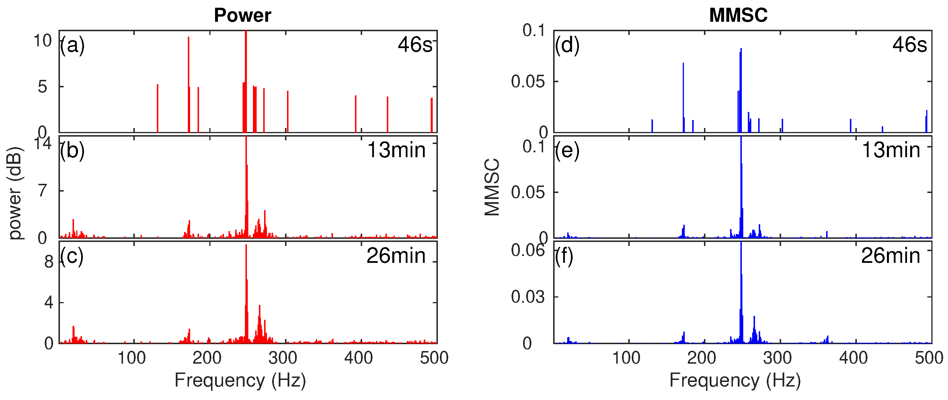
2.2. Temporal Coherence Analysis of Ship Tonal Sound Using MMSC

The persistent narrowband tonal sounds radiated from ship machinery constitute highly coherent sound fields that can be quantified via MMSC. Because the tonal signals have energies that are confined to relatively narrow frequency bands centered at certain frequencies over long time durations, the PSD in adjacent time periods will be highly correlated at those tonal frequencies. First, the magnitude-squared coherence [45,46] between two adjacent beamformed time-windowed signals is calculated,
M S C x w , x w + 1 ( f , θ i ) = | P x w , x w + 1 ( f , θ i ) | 2 P x w , x w ( f , θ i ) P x w + 1 , x w + 1 ( f , θ i ) ,
where x w ( t , θ i ) and x w + 1 ( t , θ i ) represent signals in two adjacent time windows w and w + 1 in bearing θ i . Then MMSC between beamformed adjacent time-windowed signals in one data unit is calculated to show the averaged coherence,
M M S C ( f , θ i ) = 1 N 1 w = 1 N 1 M S C x w , x w + 1 ( f , θ i ) ,
where N is the total window number in one data unit.
The MMSC values and relative bearings are extracted at each frequency for prominent peaks in M M S C ( f , θ ) within each data unit. Prominent peaks with high MMSC values are identified via a peak detector. Note that, at each frequency, multiple peaks whose bearing separations are greater than the corresponding beamwidths can be extracted in order to account for multiple distinct targets that may generate tonal signals at the same frequency and at the same time. In this work, only information for the largest two MMSC peaks are output at each frequency. Persistent tonal signals can be identified by concatenating the results from consecutive data units within the recording time interval. Furthermore, a 2D image of MMSC values as a function of bearing and time can reveal the bearing-time trajectories of potential machinery targets. We provide estimates of tonal sound signature for each target by averaging detected signals’ MMSC-frequency and power-frequency distributions along their corresponding bearing-time trajectories.

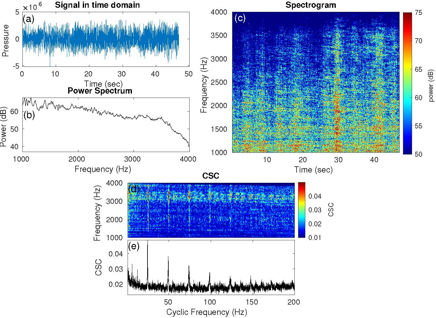
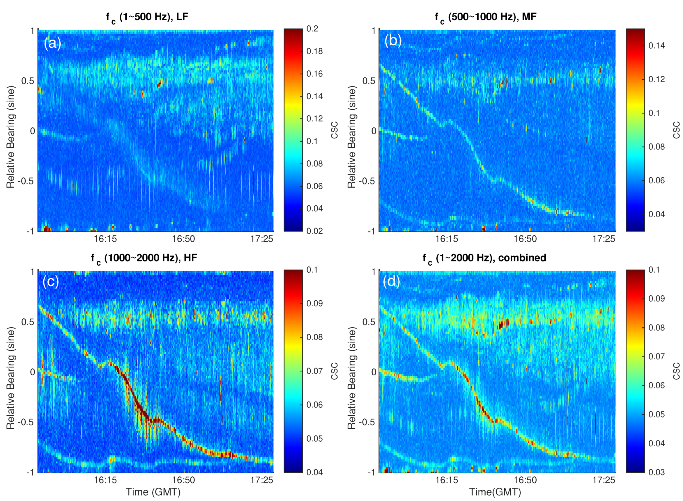
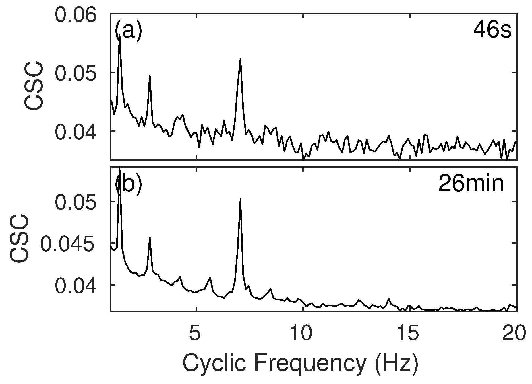
2.3. Spectral Coherence Analysis of Ship Cavitation Noise Using CSC

Rotating machinery, such as a ship’s propeller, generate acoustic signals that are cyclostationary, which have hidden periodicities or repetitive patterns, for instance, periodic energy flows [41,42]. These signals are spectrally coherent, due to interfering spectral components that are spaced apart by fundamental and harmonic frequencies, comprising Fourier series components. The CSC analysis provides an approach for determining the cyclic frequencies. It is based on cyclic spectral correlation that is defined as the Fourier transform of the cyclic auto-correlation function [43],
S x α ( f ) = R x α ( τ ) e i 2 π f τ d τ
R x α ( τ ) = x ( t τ 2 ) x * ( t + τ 2 ) e i 2 π α t d t
where R x α ( τ ) is the cyclic auto-correlation function of signal x ( t ) at cyclic frequency α , and S x α ( f ) is the corresponding cyclic spectral correlation.
Among numerous cyclic spectral correlation estimators, the fast spectral correlation S x F a s t ( α , f ) [42] has been shown to provide fast computation and better statistical performance. It is calculated, as follows,
S x F a s t ( α , f ) = p = 0 P S x ( α , f ; p ) p = 0 P R w ( α p Δ f ) R w ( 0 )
S x ( α , f k ; p ) = 1 K w 2 F s i = 0 K 1 X S T F T ( i , f k ) X S T F T ( i , f k p ) * e j 2 π α F s ( i R + N 0 ) e j 2 π p N 0 N w
= 1 K w 2 F s D F T i α { X S T F T ( i , f k ) X S T F T ( i , f k p ) * } e j 2 π N 0 ( α F s p N w )
α = p Δ f + δ
P = N w 2 R
R w ( α ) = n = 0 N w 1 | w [ n ] | 2 e j 2 π ( n N 0 ) α F s
X S T F T ( i , f k ) = m = 0 N w 1 x [ i R + m ] w [ m ] e j 2 π m f k F s
where S x ( α , f k ; p ) represents “scanning spectral correlation” which estimates spectral correlation from the Discrete Fourier Transform of the interactions between the STFT coefficients in frequency bins f k and f k p , not necessarily spaced apart by exact α but by p Δ f , which is the closet frequency bin to α with some residue δ in order to smoothly envelope the wave packet. Here, R w ( α ) is the window kernel from window function w with central time index at N 0 , K is the total number of windows, each of sample length N w , R is the window moving length, and P is the maximum value of p.
By applying this estimator on beamformed signal x θ i , the beamformed spectral coherence γ x θ i can be obtained,
S x θ i ( α , f c ) = S x θ i F a s t ( α , f c )
γ x θ i ( α , f c ) = S x θ i ( α , f c ) S x θ i ( f c ) S x θ i ( f c α ) .
Subsequently, ( C S C α f c ) θ i and ( C S C α ) θ i are obtained as the magnitude of γ x θ i and mean magnitude across carrier frequency f c , respectively,
( C S C α f c ) θ i = | γ x θ i ( α , f c ) |
( C S C α ) θ i = 1 N f c f c ( C S C α f c ) θ i
where ( C S C α f c ) θ i is the two-dimensional magnitude of beamformed cyclic spectral coherence function, depending on cyclic frequency α and carrier frequency f c while ( C S C α ) θ i reveals its overall dependence on cyclic frequency α .
The analysis proceeds by first setting the carrier frequency range f c for each beamformed signal x θ i , depending on the array aperture. Next, ( C S C α f c ) θ i are calculated in each data unit as a function of carrier frequency f c , cyclic frequency α and relative bearing θ i . f c is next averaged out to obtain ( C S C α ) θ i as a function of cyclic frequency and bearing. For each bearing, maximum CSC value is extracted except for zero cyclic frequency. By concatenating the maximum CSC values from consecutive data units over the recording interval, we obtain C S C m a x distribution in bearing-time space that can reveal bearing-time trajectories of potential targets whose propellers generate amplitude-modulated cavitation noise. Then propeller rotation signatures are obtained in terms of ( C S C α ) m e a n by averaging C S C α along corresponding bearing-time trajectories. The signature for each ship contains a combination of harmonics of the fundamental shaft rotation frequency that includes the propeller blade-pass rotation frequency.

2.4. Ship Sound’s Energetics Analysis with PSD

Engine-powered ships tend to be acoustically energetic, generating both cavitation broadband and machinery narrowband sounds distributed over a wide range of frequencies and over long time durations, regardless of ship propulsion mechanism. Here, we quantify the average received power spectral density of acoustically energetic targets,
P θ i ( f ) = F { R x θ i x θ i ( t ) }
P θ i m e a n = 1 N f j = 1 N f P θ i ( f j ) ,
where P θ i ( f ) is the spectral density of the beamformed signal x θ i that is obtained from Fourier transform of its auto-correlation R x θ i x θ i function following the Wiener–Khinchin theorem, and P θ i m e a n is the mean PSD averaged across broad discrete frequency bands quantified by N f . The Welch’s averaged modified periodogram method [50,51] is utilized to calculate spectral estimation.
A peak detector is first applied on P θ m e a n to output bearings containing acoustic signals with prominent mean received PSD within each data unit. By concatenating results from multiple data units over the recording time interval, the bearing-time trajectories of potential ships can be identified and tracked. The mean received PSD signatures ( P ) m e a n can be obtained by further averaging the PSD across time and bearing for each ship.

3. Results

Here, we provide an analysis of the underwater sound radiated by several ocean vessels and received on the towed coherent hydrophone array for a representative subset of data recorded on 26 February 2014 during the NorEx2014 Experiment. The ships present in the region include three fishing vessels, a research vessel, a search and rescue vessel, and a cargo ship (see Section 3.3.3) with distances from the array center ranging from 200 m to 200 km and speeds between 0.5 knots to 13 knots, as verified by GPS data from AIS database for the region. The identity of these ships are provided in Table 3 of [33].
Machinery tonal sounds, cyclostationary cavitation noise, and general broadband power levels for these ships are detected and analyzed by applying the MMSC, CSC, and PSD methods, respectively, to beamformed coherent hydrophone array data. We provide acoustic signature characterization along with estimated bearing-time trajectories for each vessel that include (a) key tonal frequencies for ship machinery; (b) propeller shaft rotation frequency, blade-pass frequency and propeller blade number;and, (c) received mean PSD averaged across specific broad bandwidths to quantify ship radiated sound energetics.

3.1. Beamform Analysis of Coherent Hydrophone Array Data

Raw pressure-time series data from 64 hydrophones each in the LF, MF, and HF subapertures are separately beamformed into 100 bearings spanning forward- to back-endfire directions relative to the array aperture axis and center to form beam-time data images. The beamforming of coherent hydrophone array data enhances signal-to-noise ratio (SNR) by rejecting noise outside of the signal beam, and provides signal bearing estimation. A comparison of single omnidirectional hydrophone spectrogram with beamformed spectrogram for a given bearing within a 46.8 s data unit is shown in Figure 1. Spectrograms in Figure 1 reveal both narrowband tonal signals and broadband cavitation noise generated by passing ocean vessels and own tow ship, as well as other other sounds.
The PSD is next calculated for each beam-time signal. An example is plotted in Figure 2a–c as a function of signal bearing and frequency. This figure reveals that the narrowband tonal signals are spread over wider range of beams than large bandwidth broadband signals, especially at frequencies that are significantly lower than the array cut-off frequency in each sub-aperture.

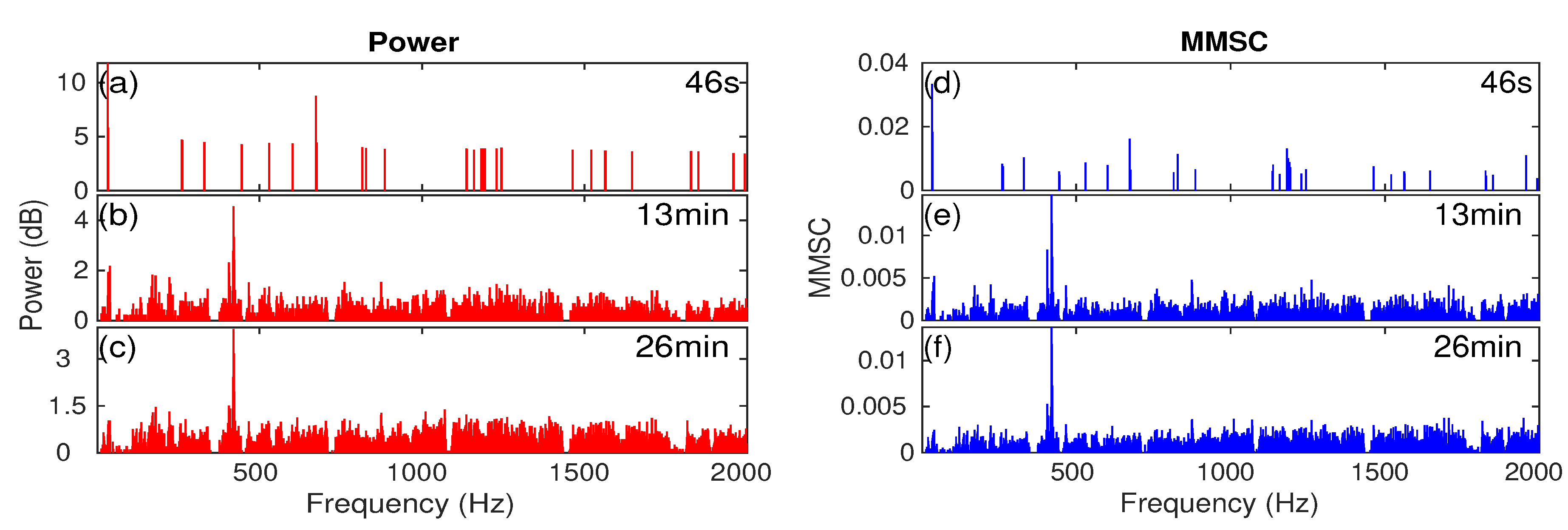
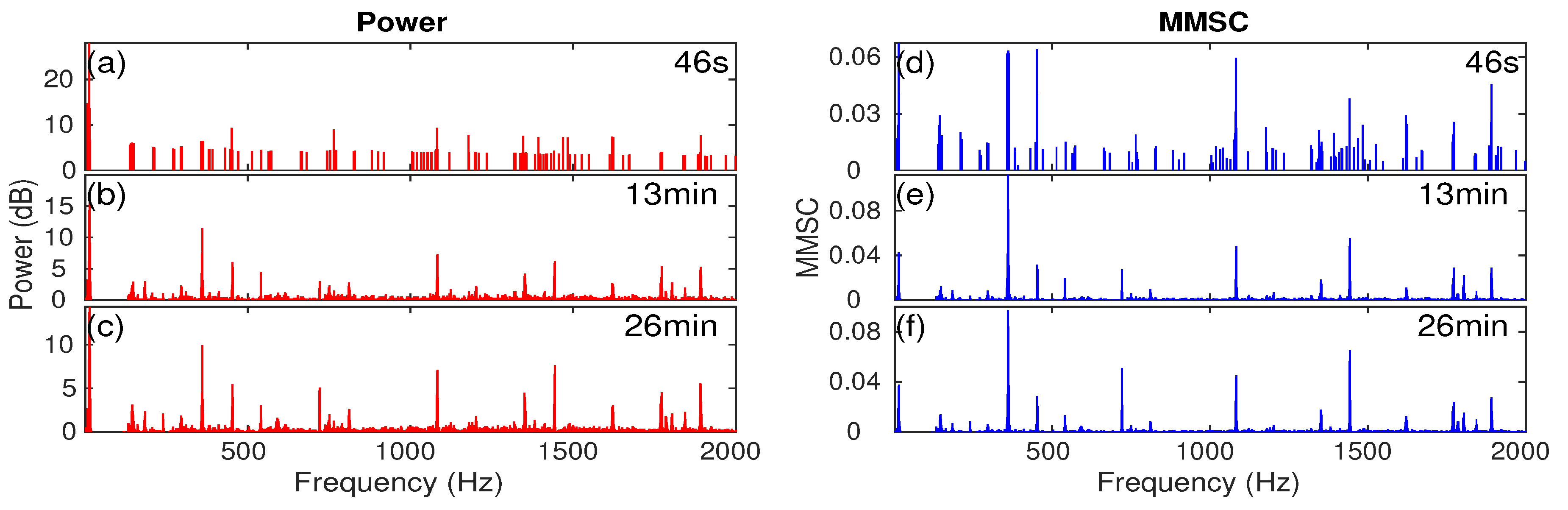
3.2. Machinery Tonal Sound Analysis via MMSC

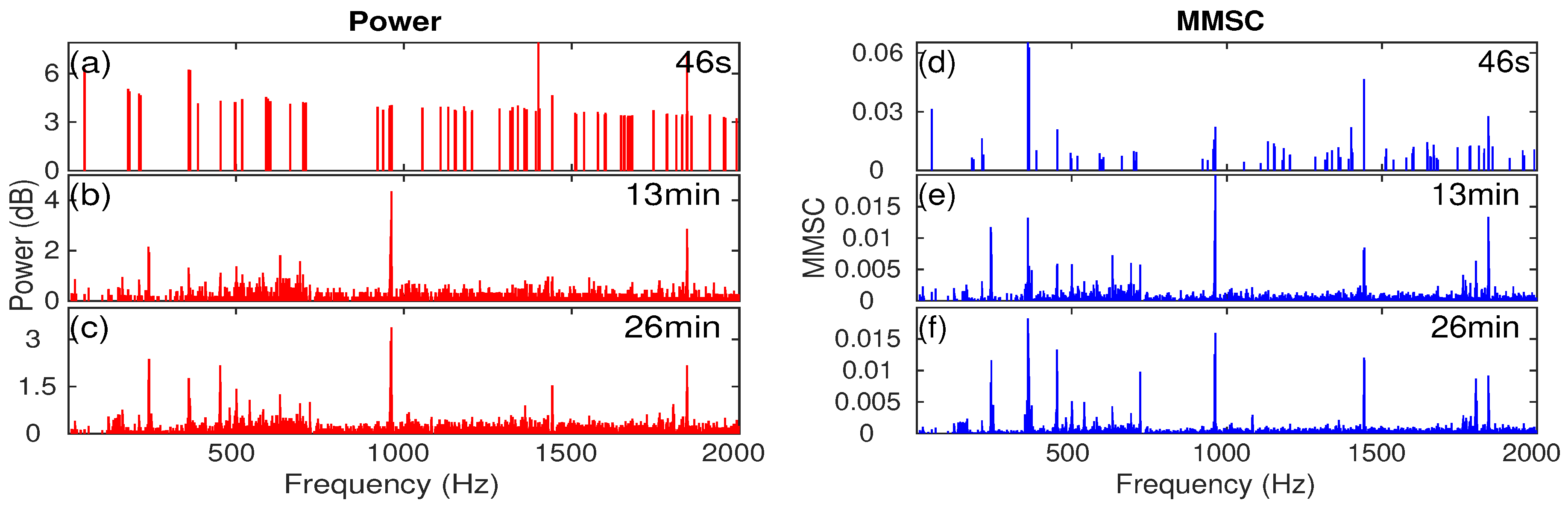
3.2.1. Comparing MMSC with Conventional Power Spectrum Analysis

An advantage of MMSC for tonal sound analysis is that it detrends the data compared to traditional power spectrum analysis, as illustrated in Figure 3. The conventional power spectrum applied to a beamformed signal from our dataset is plotted in linear and log scales in Figure 3a–b, respectively, and contains narrowband tonal signals embedded in ocean acoustic background ambient noise. The latter decays with increasing frequency. The MMSC output that is shown in Figure 3c, on the other hand, efficiently detrends the data enabling tonal signals to be enhanced above the background levels. Only a single threshold is needed for tonal peak detection via MMSC analysis. In contrast, conventional power spectrum analysis would require detrending the background before peak detection, or application of a local moving peak detector. The MMSC reveals many more tonal signals than can be observed using the conventional power spectrum analysis.
Next, MMSC analysis is applied to beam-time data with an example plotted in Figure 2d–f separately for data from each subaperture. The MMSC efficiently detrends the background enabling detection of tonal signals with high SNR when compared to power spectrogram analysis shown in Figure 2a–c. Broadband noise has been greatly suppressed using MMSC analysis, enabling better tonal peak detection.

3.2.2. Bearing Estimation of Targets from MMSC

Consecutive data files, each 46.8 s long, received between 15:44:00 and 17:29:24 GMT on 26 February during NorEx2014 and beamformed into 100 azimuthal directions are analyzed here using MMSC. The MMSC processing data unit is 7.8 s with 50% overlap between adjacent data units. Within each data unit, the MSC is calculated for 0.97 s duration signal portions using 1024 points window with 512 points overlap.
The MMSC values of peak detections in bearing-time space are extracted and plotted in Figure 4a–c separately for the LF, MF, and HF subapertures in frequency ranges 1–500 Hz, 100–1000 Hz, and 1000–2000 Hz, respectively. Figure 4d shows the MMSC values in corresponding bearing-time distributions within 1–2000 Hz combined from all three subapertures. These MMSC distributions reveal bearing-time trajectories of seven targets, of which five have been identified as distant ships with locations verified by GPS, labelled as M1, M5, M6, M9, and M12 (see Table 3 of [33]).
The relative bearings of these ships from the receiver array axis, as calculated from their GPS data, are plotted in Figure 5a. Their speeds and distances from the receiver array center are plotted in Figure 5c–d. Over the 1 h and 45 min analysis time period shown here, the speed and range of each ship remains relatively stable, between 0.5 knots to 13 knots and 200 m to 196 km, respectively, depending on the ship. The GPS-derived bearings of the five ships are overlain on the MMSC beam-time image in Figure 5b and show very good correspondence with bearing-time trajectories of acoustic MMSC detections. The remaining prominent MMSC detections are located in the forward endfire direction (relative bearing sin ( θ ) = 1 ) and between sin ( θ ) = 0.59 to sin ( θ ) = 0.7 . These correspond to detections of our own tow ship sound at the receiver array arriving directly from the tow ship or after one bottom bounce or reflection from the sea floor, respectively. As expected, the direct tonal arrivals from our own tow ship located in forward endfire direction sin ( θ ) = 1 have the largest MMSC values in every frequency subband shown in Figure 4a–d and in some cases very close to perfect coherence of 1.
Combining the results from multiple subapertures and subbands in Figure 4d is advantageous for tracking all five distant ships’ bearing-time trajectories, since they have prominent MMSC values in at least one, if not more, frequency sub-bands. The MMSC detections in MF subaperture 100–1000 Hz subband have consistently good SNR, as shown in Figure 4b for all ships. In contrast, vessels M5, M6, and M9 have much lower MMSC values in the HF subaperture 1000–2000 Hz subband (Figure 4c) indicating that the tonal signals for these ships at the higher frequencies are less coherent. Furthermore, vessels M1 and M12 have undetectable coherent tonals in this HF frequency subband. For M1, both low frequency mechanical vibration due to low speed and high-frequency signal dissipation due to long-range propagation cause the received tonal signals from this ship to be restricted to <1000 Hz frequency. Because M12 is a cargo ship with large propellers, its low frequency engine rotation can provide high speeds [9] resulting in negligible high frequency tonals, and it will be discussed further in Section 3.3.
The corresponding power and frequency of MMSC peak detections are plotted in Figure 6 and Figure 7, respectively, as a function of bearing and time. These images reveal that the tonal signals detections are highly energetic in most frequency subbands when detected via MMSC calculations. For instance, vessels M5, M6, and M9 have tonals that are not highly coherent in the HF 1000–2000 Hz subband, but they are energetic.

3.2.3. Individual Ship’s Tonal Sound Signature in Different Time Period

Here, the tonal sound signatures of distant ships and our own tow ship are derived. The mean MMSC and log-transformed average power calculated from detected tonal sound signals in each ship’s bearing-time trajectories are plotted as a function of frequency in Figure 8 for ship M1 and in Appendix A for the other distant ships and our own tow ship. Results are shown for three averaging time periods of 46 s, 13 min and 26 min in the time frame from 16:15:46 to 16:42:40 GMT. For own tow ship, the tonal sound signatures are presented for (a) the direct arrival in forward endfire sin ( θ ) = 1 , direction (b) seafloor reflected, averaged over sin ( θ ) = 0.59 to sin ( θ ) = 0.7 relative bearing range, and (c) seafloor reflected in the sin ( θ ) = 0.68 relative bearing direction. These results show that some tonals are highly consistent over long time periods, while others tend to fade over time.

3.3. Propeller Noise Analysis via CSC

3.3.1. Received Broadband Cavitation Noise Overview

For illustration, we first demonstrate the result of CSC analysis applied to a beamformed signal to examine the cyclostationary broadband cavitation noise generated by an ocean vessel. The beamformed time-domain signal, spectrum, and spectrogram are shown in Figure 9a–c. The signals CSC distribution in cyclic and carrier frequency α f domain and mean CSC distribution in cyclic frequency α domain, obtained by averaging across carrier frequency f are shown in Figure 9d–e. This subplot reveals the harmonic group of frequencies associated with the propeller shaft and blade rotation of a ship, with a fundamental frequency of 6.17 Hz.

3.3.2. Bearing-Time Trajectory Estimation for Targets from CSC Analysis

Here, the CSC analysis is applied to multiple data files over our analysis time period in order to detect bearing-time trajectories of potential ships with cavitation noise. The CSC calculations are conducted on the 100 individually beamformed signals spanning azimuthal angles sin ( θ ) = 1 to sin ( θ ) = 1 relative to the array axis. Each CSC processing data unit is again chosen to be 7.8 s with 50% overlap between adjacent data units. Within each data unit, the CSC is calculated using 256 point window with 216 point overlap to cover cyclic frequency components up to 100 Hz.
The maximum CSC values extracted from peak detection are plotted in bearing-time space in Figure 10a–c for the LF, MF, and HF subapertures, respectively, corresponding to carrier frequency ranges of 1–500 Hz, 500–1000 Hz, and 1000–2000 Hz, respectively. Figure 10d shows maximum CSC distribution of signals within 1–2000 Hz carrier frequencies combined from all three subapertures. These maximum CSC bearing-time images reveal the bearing-time trajectories of six cyclostationary ship sound sources. Four of these are the GPS-verified distant ships M5, M6, M9, and M12, while the remaining two are due to our own tow ship direct-arrival and seafloor-reflected signals. The bearing-time trajectories of M6 and M9 are clear and can be tracked over most of the analysis time period, while that of M12 is clearly visible only at the beginning, and that of M5 is faint throughout. Best results are obtained in the 500–1000 Hz frequency range from CSC analysis of MF subaperture data, with CSC values for distant ship noise standing above the background and well confined within the bearing of these ships, Figure 10b. The CSC values are the largest in the 1000–2000 Hz frequency range, Figure 10c. Besides cavitation noise from ships, Figure 10a–d also contain other patterned signals whose maximum CSC values stand above the background levels. These patterned signals are due to other ocean sound sources such as marine mammal vocalizations, that may be repetitive. However, unlike ship propeller cavitation noise, these other sound sources do not generate patterned signals over a long enough time duration or with large enough repetition rates to form clear and continuous bearing-time trajectories. Examples of CSC analysis applied to patterned signals from marine mammal vocalizations are provided in Section 3.5.
The vessel M1’s bearing-time trajectory cannot be clearly distinguished in Figure 10a–d. This is because M1 is located roughly 192.4 km from the receiver array where high frequency signal components from this ship are significantly attenuated due to propagation and absorption losses in the ocean. Furthermore, its speed of approximately 0.78 knots is low so that its propellers may only generate low-frequency cavitation noise. The only dominant signal from the previous MMSC analysis for ship M1 is a 250 Hz narrowband tonal, which is likely to get averaged out over the wide carrier frequency ranges used in the CSC analysis for Figure 10. To focus on the 250 Hz tonal for ship M1 and potential cavitation noise, we reanalyze the data via CSC by averaging the carrier frequency only within 200–300 Hz carrier frequency range, using data from the LF subaperture in Figure 11. The bearing-time trajectory of ship M1 can now be clearly distinguished from the background. This 200–300 Hz carrier frequency subband analysis also enhances the bearing-time trajectory of ship M12. This indicates that the received propeller cavitation noise from both vessels are mostly present only within the 200–300 Hz frequency subband in the analysis time period. The two methods for ship noise analysis, MMSC, and CSC, are complementary, since tonal frequencies identified using MMSC can provide useful inputs for fine-tuning carrier frequency ranges in the CSC approach.

3.3.3. Individual Ship’s CSC Signature in Different Time Period

The CSC signatures of distant ships and our own tow ship due to cyclostationary cavitation noise from propeller rotation are shown in Figure 12, Figure 13, Figure 14 and Figure 15. They contain harmonic groups of frequencies that are characteristic of each ship. They are calculated as mean CSC distributions averaged across each ship’s bearing-time trajectory. The CSC signatures are averaged over two time frames, 46 s or a single data file file duration, and 26 min. over multiple data files. Table 1 shows the analysis carrier frequency ranges and time periods for different vessels to best reveal their propellers’ rotation characteristics.
From each CSC signature plot, the fundamental propeller shaft frequency is obtained as the first order harmonic. The blade-pass frequency is obtained as the harmonic with an abrupt magnitude increase in the harmonic series. The propeller blade number (or number of blades on the propeller) is given by the harmonic order of the blade-pass frequency or equivalently the ratio of the blade-pass frequency to the shaft frequency. Table 2 lists the derived CSC signature frequencies of distant vessels and our own tow ship, along with speed and range information from GPS data. The estimated propeller blade number for our own tow ship, RV KNORR, exactly matches that shown in pictures of its propeller [52].
For our own tow ship, CSC signatures of seafloor reflected arrivals (Figure 15c–d) have much higher SNR than that for the direct arrivals (Figure 15a–b), especially in the 46 s CSC signatures. Additionally, the relative magnitude difference between 5th and 4th harmonic is higher in the CSC signatures for seafloor reflected arrivals than direct arrivals, which can better reveal the blade-pass frequency. Besides the prominent harmonic group with fundamental frequency at 10.03 Hz, there are also other less prominent spikes that may come from tow ship’s other onboard rotating machinery besides the propeller.

3.4. General Energy Analysis of Ship-Radiated Underwater Sound via PSD

Here, we quantify the energetics of the received signals from distant ships and own tow ship by calculating the PSD averaged across broad bandwidths for beamformed signals. Each beamformed signal processing unit is again chosen to be 7.8 s with 50% overlap between adjacent data units, with PSD calculated using 1024 points window with 512 points overlap. The PSD is next averaged across several frequency bands and the power output across beams are stacked over multiple data files in our recording time interval. This image reveals the bearing-time trajectories of acoustically energetic sound sources.
The prominent mean-PSD distributions in bearing-time space of received signals from HF, MF and LF subapertures corresponding to averaging frequency ranges 1000–2000 Hz, 100–1000 Hz, and 1–500 Hz, respectively, are shown in Figure 16a–c. With the exception of M1, the bearing-time trajectories of all other distant ships and our own tow ship are clearly visible and can be followed. Previous acoustic analysis of vessel M1 indicates both its received tonal signal and cavitation noise are within 200–300 Hz. When the PSD averaging bandwidth for data from the LF subaperture is confined to 200–300 Hz instead, the output clearly shows the bearing-time trajectory of vessel M1, in addition to increasing the SNR for vessels M5 and M12. We find this 200–300 Hz frequency range to be ideal for analyzing ship radiated underwater sound energetics, since all of the vessels studied here can be detected with significantly high SNR in output mean PSD. Other sound sources are also present in this frequency range, but weaker, and are unlikely to be mechanized ships, since they do not generate tonal or cyclostationary propeller type signals.

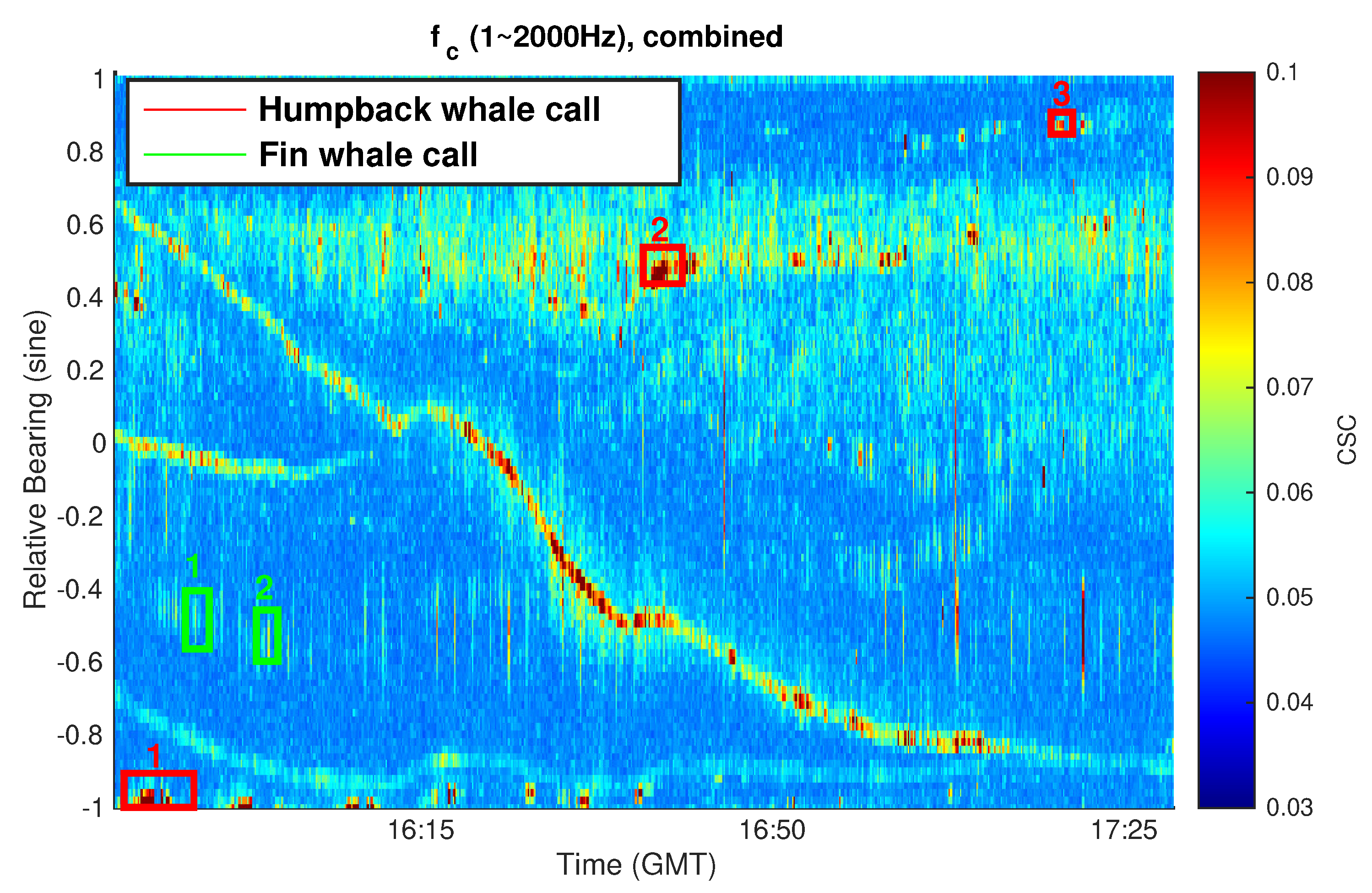
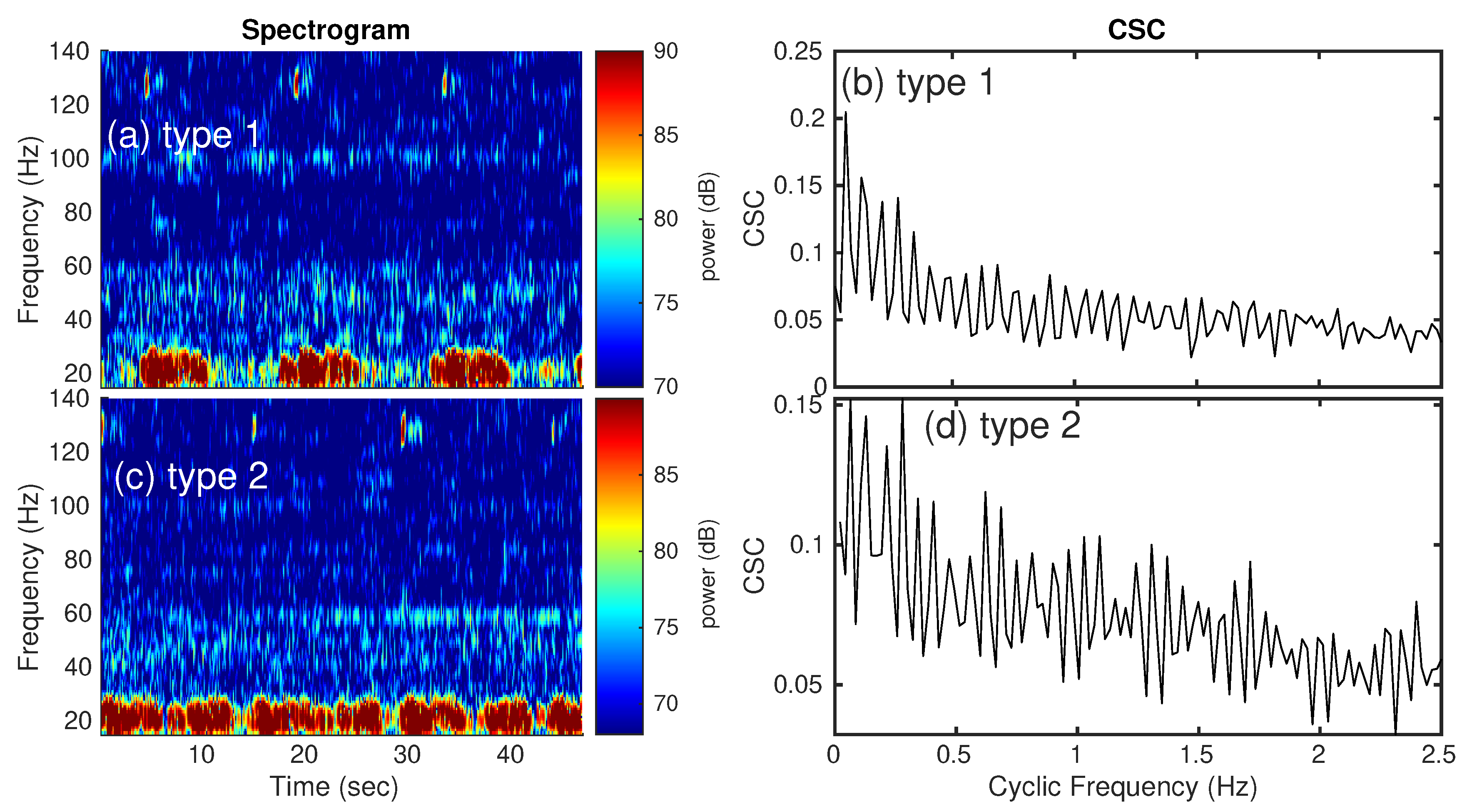
3.5. Marine Mammal Vocalization Analysis via CSC

Here, we provide an analysis of marine mammal vocalizations from fin whales and humpback whales using the CSC-based method. We show that this approach is extremely useful for estimating the inter-pulse intervals in repetitive call types, such as fin 20 Hz pulses, and minke and humpback whale buzzes, as well as time intervals between pulse or buzz train sequences. Figure 17 shows an example of the maximum CSC distribution obtained from combining the results from analysis in the LF, MF, and HF subapertures. In addition to ship radiated underwater sound within fairly continuous bearing-time trajectories, there are also some other discrete bearing-time patterns present in the image. These discrete patterns are due to marine mammals vocalizations. For example, several different humpback whale vocalizations types are enclosed in the red box, while two different fin whale call types are enclosed in the green box.
Figure 18 and Figure 19 plot the beamformed spectrograms and corresponding CSC distributions for these various marine mammal call types. The CSC spectra show various peaks due to the repetitive nature of the marine mammal vocalizations. The inter-pulse-train and inter-pulse intervals are estimated as the inverse of the cyclic fundamental and first recurring peak frequencies, respectively, of two harmonic groups and provided in Table 3. The estimated inter-pulse or inter pulse-train intervals match well with those that are shown in the corresponding spectrogram.

4. Discussion

We have applied and demonstrated three approaches for ship radiated underwater sound analysis with a large aperture coherent hydrophone array, providing robust approaches for ship detection, bearing-time estimation, and acoustic signature characterization. The three methods each focus on a different aspect of ship sound; MMSC for narrowband tonal machinery sound, CSC for cyclostationary broadband cavitation noise amplitude-modulated by propeller rotation, and broadband energetics for general high-powered mechanized ship sound. The signatures of their radiated underwater sound have been quantified in terms of tonal frequency components, propeller rotation and shaft frequencies, and number of propeller blades, as well as mean radiated power over broad bandwiths for several different types of ocean vessels. The approaches are applied to beamformed data spanning 0 to 360 horizontal azimuths, enabling the simultaneous detection and characterization of multiple engine powered ships at a variety of bearing and ranges as far as 200 km from the coherent hydrophone array.
The three approaches are independent, but they can complement each other to enhance ship radiated underwater sound analysis. For instance, we found ship M1 that was very far away, on average 193 km from our coherent hydrophone array and travelling at low speeds, did not generate a clear bearing-time trajectory in the output from direct application of the CSC and PSD methods. We were able to enhance the results in these methods for ship M1 by using information from the MMSC approach that showed this ship had only one detectable narrowband tonal signal at the low frequency of 250 Hz. This knowledge was used to reduce and confine the frequency range for averaging in the other two methods, which are the cyclic frequency range in CSC and the PSD averaging bandwidth, to focus analysis to the low frequency 200–300 Hz range, making ship M1 detectable with improved SNR in these methods after the modification. A hybrid approach can be developed in the future, combining these three approaches that use information from one approach to automatically optimize the parameters in the other two approaches to ensure that ship detection and characterization in terms of narrowband tonal frequencies, propeller, and shaft cyclic frequencies, as well as broadband energetics is achievable directly, rather than via manual feedback.
From the study conducted here, we can summarize the usefulness and advantages, as well as some challenges, which are associated with the three approaches for ship radiated underwater sound analysis with a coherent hydrophone array. We find the MMSC approach is extremely efficient in detecting narrowband tonal signals even when a ship is very far away (approximately 200 km), so long as the tonal is sufficiently energetic within the small bandwidth compared to adjacent frequencies. Furthermore, MMSC detrends the data, enhancing the detection of low energy tonals that may be drowned in the noise in traditional power spectrum methods, as we have shown.
In the CSC approach implemented here, the peak cyclic frequency component is output at each point in beam-time space in order to generate the bearing-time trajectories for multiple ships without any prior information. Detailed propeller rotation signatures of multiple ships are then estimated by averaging CSC distributions along corresponding bearing-time trajectories for each ship. This approach is extremely useful, since no a priori information is needed for finding acoustic signature and can be applied to analyze multiple ships simultaneously. Previous publications [37,40] based on measurements with a single hydrophone or sparse array typically provide information for a single ship only that is acoustically dominant and in close proximity to the sensor. Prior information regarding ships’ signatures would be necessary for tracking two more ships in sparse sensor measurements since those approaches are directly dependent on knowledge of harmonic components for cross-correlation in direction of arrival estimation [37,40].
The energy-based method here can rapidly detect and provide bearing-time trajectories containing ships. However, it cannot provide detailed time-frequency characteristics of ship sound or propeller characterization, and it may need to be fine-tuned in order to prevent missed detection. The energy-based approach is easy to implement, which makes it useful for rapidly estimating ship bearing-time trajectories.
Finally, analysis of patterned marine mammal vocalizations using the CSC-based method are provided. The call rates and intervals for click sequences for several repetitive call types from humpback and fin whales have been provided. The derived CSC distribution reveal the periodicities in energy flow of the marine mammal vocalizations that can be used for classifying the call types.

5. Conclusions

Three approaches for ship long-range automatic detection, acoustic signature characterization, and bearing-time trajectory estimation have been developed and applied, each focusing on a different aspect of a ship’s radiated underwater sound received on a large-aperture densely-sampled coherent hydrophone array. Ship radiated underwater sound has been analyzed from multiple ships with significantly enhanced signal-to-noise ratios after beamforming, enabling detection and acoustic signature characterization for each ship, from long ranges and distributed over instantaneous continental-shelf scale regions. The three approaches, Mean Magnitude-Squared Coherence (MMSC), Cyclic Spectral Coherence (CSC), and broadband energetics, were applied to beamformed data from roughly two hours of acoustic recordings of the 160-element coherent hydrophone array that was deployed in the Norwegian Sea during an experiment in February 2014. Six GPS-verified ocean vessels have been automatically detected and their acoustic signatures characterized, located at a variety of bearings and ranges out to 200 km from the coherent hydrophone array, with speeds ranging from 0.5 knots to 13 knots. We have quantified the machinery tonal sound signature, propeller rotation signature, and ship broadband energetics for each of these six engine-powered ocean vessels that can be employed for automatic classification. We also demonstrate automatic detection, bearing-time estimation, and temporal characterization of repetitive marine mammal vocalizations in recorded coherent hydrophone array data using the CSC-based method.

Author Contributions

Data analysis, reduction, and interpretation was conducted primarily by C.Z., with contributions from S.G.S. and H.M.-K.; C.Z. and P.R. wrote the paper; research was directed by P.R. All authors have read and agreed to the published version of the manuscript.

Funding

This research was funded by United States Office of Naval Research (ONR) grant number N00014-20-1-2026 and the United States National Science Foundation grant number OCE-1736749.

Acknowledgments

We thank Nicholas Makris of Massachusetts Institute of Technology and Olav Rune Godo of Norwegian Institute of Marine Research—Bergen for leading the experiment and data collection for the NorEx2014 Experiment, which was funded by ONR and IMR-Bergen. We also thank John Kaplan, Anna Kaplan of Northeastern University, Alessandra Tesei of CMRE-Italy, Tvika Feldman and Moshe Solomon from Tel Aviv University, and Nicholas Makris for discussions on the topic.

Conflicts of Interest

The authors declare no conflict of interest.

Appendix A. Individual Ship’s Tonal Sound Signature in Different Time Period

The tonal sound signature of remaining ships from MMSC analysis in Section 3.2.3 are provided here.
Figure A1. Tonal sound signatures of vessel M5 in averaging time period (a,d) 46 s, (b,e) 13 min, and (c,f) 26 min.
Remotesensing 12 03731 g0a1
Figure A2. Tonal sound signatures of vessel M6 in averaging time period (a,d) 46 s, (b,e) 13 min, and (c,f) 26 min.
Remotesensing 12 03731 g0a2
Figure A3. Tonal sound signatures of vessel M9 in averaging time period (a,d) 46 s, (b,e) 13 min, and (c,f) 26 min.
Remotesensing 12 03731 g0a3
Figure A4. Tonal sound signatures of vessel M12 in averaging time period (a,d) 46 s, (b,e) 13 min, and (c,f) 26 min.
Remotesensing 12 03731 g0a4
Figure A5. Tonal sound signatures of own tow ship KNORR’s direct arrival signals within relative bearing sin ( θ ) = 1 in forward endfire direction over averaging time period (a,d) 46 s, (b,e) 13 min, and (c,f) 26 min.
Remotesensing 12 03731 g0a5
Figure A6. Tonal sound signatures of own tow ship KNORR’s seafloor-reflected signals averaged over relative bearing sin ( θ ) = 0.5 to sin ( θ ) = 0.7 in averaging time period (a,d) 46 s, (b, e) 13 min, and (c,f) 26 min.
Remotesensing 12 03731 g0a6
Figure A7. Tonal sound signatures of own tow ship KNORR’s seafloor-reflected signals within relative bearing sin ( θ ) = 0.68 over averaging time period (a,d) 46 s, (b,e) 13 min, and (c,f) 26 min.
Remotesensing 12 03731 g0a7

References

  1. Bergmann, P.G.; Major, J.; Wildt, R. Physics of Sound in the Sea; Gordon and Breach: New York, NY, USA, 1968. [Google Scholar]
  2. Arveson, P.T.; Vendittis, D.J. Radiated noise characteristics of a modern cargo ship. J. Acoust. Soc. Am. 2000, 107, 118–129. [Google Scholar] [CrossRef] [PubMed]
  3. Bruno, M.; Chung, K.; Salloum, H.; Sedunov, A.; Sedunov, N.; Sutin, A.; Graber, H.; Mallas, P. Concurrent use of satellite imaging and passive acoustics for maritime domain awareness. In Proceedings of the 2010 International Waterside Security Conference (WSS), Carrara, Italy, 3–5 November 2010. [Google Scholar]
  4. Chung, K.W.; Sutin, A.; Sedunov, A.; Bruno, M. DEMON acoustic ship signature measurements in an urban harbor. Adv. Acoust. Vib. 2011, 2011, 952798. [Google Scholar] [CrossRef] [Green Version]
  5. Fillinger, L.; Sutin, A.; Sedunov, A. Acoustic ship signature measurements by cross-correlation method. J. Acoust. Soc. Am. 2010, 129, 774–778. [Google Scholar] [CrossRef] [PubMed]
  6. Leal, N.; Leal, E.; Sanchez, G. Marine vessel recognition by acoustic signature. ARPN J. Eng. Appl. Sci. 2015, 10, 9633–9639. [Google Scholar]
  7. Ogden, G.L.; Zurk, L.M.; Jones, M.E.; Peterson, M.E. Extraction of small boat harmonic signatures from passive sonar. J. Acoust. Soc. Am. 2011, 129, 3768–3776. [Google Scholar] [CrossRef] [Green Version]
  8. Wales, S.C.; Heitmeyer, R.M. An ensemble source spectra model for merchant ship-radiated noise. J. Acoust. Soc. Am. 2002, 111, 1211–1231. [Google Scholar] [CrossRef]
  9. Urick, R.J. Principles of Underwater Sound, 3rd ed.; Peninsula Publising: Los Atlos, CA, USA, 1983. [Google Scholar]
  10. Wenz, G.M. Acoustic ambient noise in the ocean: Spectra and sources. J. Acoust. Soc. Am. 1962, 34, 1936–1956. [Google Scholar] [CrossRef]
  11. Makris, N.C.; Ratilal, P.; Symonds, D.T.; Jagannathan, S.; Lee, S.; Nero, R.W. Fish population and behavior revealed by instantaneous continental shelf-scale imaging. Science 2006, 311, 660–663. [Google Scholar] [CrossRef]
  12. Makris, N.C.; Ratilal, P.; Jagannathan, S.; Gong, Z.; Andrews, M.; Bertsatos, I.; Godø, O.R.; Nero, R.W.; Jech, J.M. Critical population density triggers rapid formation of vast oceanic fish shoals. Science 2009, 323, 1734–1737. [Google Scholar] [CrossRef] [Green Version]
  13. Wang, D.; Garcia, H.; Huang, W.; Tran, D.D.; Jain, A.D.; Yi, D.H.; Gong, Z.; Jech, J.M.; Godø, O.R.; Makris, N.C.; et al. Vast assembly of vocal marine mammals from diverse species on fish spawning ground. Nature 2016, 531, 366–370. [Google Scholar] [CrossRef]
  14. Mohebbi-Kalkhoran, H.; Zhu, C.; Schinault, M.; Ratilal, P. Classifying humpback whale calls to song and non-song vocalizations using bag of words descriptor on acoustic data. In Proceedings of the 2019 18th IEEE International Conference On Machine Learning And Applications (ICMLA), Boca Raton, FL, USA, 16–19 December 2019; pp. 865–870. [Google Scholar]
  15. MacLennan, D.N.; Simmonds, E.J. Fisheries Acoustics; Springer Science & Business Media: Berlin/Heidelberg, Germany, 2013; Volume 5. [Google Scholar]
  16. Vieira, M.; Amorim, M.; Sundelöf, A.; Prista, N.; Fonseca, P.J. Underwater noise recognition of marine vessels passages: Two case studies using hidden Markov models. ICES J. Mar. Sci. 2019, 77, 2157–2170. [Google Scholar] [CrossRef]
  17. Stojanovic, M. Underwater acoustic communications. In Proceedings of the InElectro/95 International, Professional Program Proceedings, Boston, MA, USA, 21–23 June 1995; pp. 435–440. [Google Scholar]
  18. Stojanovic, M.; Preisig, J. Underwater acoustic communication channels: Propagation models and statistical characterization. IEEE Commun. Mag. 2009, 47, 84–89. [Google Scholar] [CrossRef]
  19. Dambra, R.; Firenze, E. Underwater radiated noise of a small vessel. In Proceedings of the 22nd International Congress on Sound and Vibration, Florence, Italy, 12–16 July 2015; pp. 12–16. [Google Scholar]
  20. Hildebrand, J.A. Anthropogenic and natural sources of ambient noise in the ocean. Mar. Ecol. Prog. Ser. 2009, 395, 5–20. [Google Scholar] [CrossRef] [Green Version]
  21. Merchant, N.D.; Witt, M.J.; Blondel, P.; Godley, B.J.; Smith, G.H. Assessing sound exposure from shipping in coastal waters using a single hydrophone and Automatic Identification System (AIS) data. Mar. Pollut. Bull. 2012, 64, 1320–1329. [Google Scholar] [CrossRef]
  22. Vasconcelos, R.O.; Amorim, M.C.P.; Ladich, F. Effects of ship noise on the detectability of communication signals in the Lusitanian toadfish. J. Exp. Biol. 2007, 210, 2104–2112. [Google Scholar] [CrossRef] [Green Version]
  23. Slabbekoorn, H.; Dooling, R.J.; Popper, A.N.; Fay, R.R. Effects of Anthropogenic Noise on Animals; Springer: Berlin/Heidelberg, Germany, 2018. [Google Scholar]
  24. Codarin, A.; Wysocki, L.E.; Ladich, F.; Picciulin, M. Effects of ambient and boat noise on hearing and communication in three fish species living in a marine protected area (Miramare, Italy). Mar. Pollut. Bull. 2009, 58, 1880–1887. [Google Scholar] [CrossRef]
  25. Ona, E.; Godø, O.R.; Handegard, N.O.; Hjellvik, V.; Patel, R.; Pedersen, G. Silent research vessels are not quiet. J. Acoust. Soc. Am. 2007, 121, EL145–EL150. [Google Scholar] [CrossRef] [Green Version]
  26. Mitson, R. Underwater noise radiated by research vessels. ICES Mar. Sci. Symp. 1993, 196, 147–152. [Google Scholar]
  27. Mitson, R.B.; Knudsen, H.P. Causes and effects of underwater noise on fish abundance estimation. Aquat. Living Resour. 2003, 16, 255–263. [Google Scholar] [CrossRef]
  28. Hawkins, A.D.; Pembroke, A.E.; Popper, A.N. Information gaps in understanding the effects of noise on fishes and invertebrates. Rev. Fish Biol. Fish. 2015, 25, 39–64. [Google Scholar] [CrossRef]
  29. Veirs, S.; Veirs, V.; Wood, J.D. Ship noise extends to frequencies used for echolocation by endangered killer whales. PeerJ 2016, 4, e1657. [Google Scholar] [CrossRef] [PubMed] [Green Version]
  30. Erbe, C.; Dunlop, R.; Dolman, S. Effects of noise on marine mammals. In Effects of Anthropogenic Noise on Animals; Springer: Berlin/Heidelberg, Germany, 2018; pp. 277–309. [Google Scholar]
  31. Makris, N.C.; Godø, O.R.; Yi, D.H.; Macaulay, G.J.; Jain, A.D.; Cho, B.; Gong, Z.; Jech, J.M.; Ratilal, P. Instantaneous areal population density of entire Atlantic cod and herring spawning groups and group size distribution relative to total spawning population. Fish Fish. 2019, 20, 201–213. [Google Scholar] [CrossRef] [Green Version]
  32. Garcia, H.A.; Zhu, C.; Schinault, M.E.; Kaplan, A.I.; Handegard, N.O.; Godø, O.R.; Ahonen, H.; Makris, N.C.; Wang, D.; Huang, W.; et al. Temporal–spatial, spectral, and source level distributions of fin whale vocalizations in the Norwegian Sea observed with a coherent hydrophone array. ICES J. Mar. Sci. 2019, 76, 268–283. [Google Scholar] [CrossRef]
  33. Zhu, C.; Garcia, H.; Kaplan, A.; Schinault, M.; Handegard, N.O.; Godø, O.R.; Huang, W.; Ratilal, P. Detection, localization and classification of multiple mechanized ocean vessels over continental-shelf scale regions with passive ocean acoustic waveguide remote sensing. Remote Sens. 2018, 10, 1699. [Google Scholar] [CrossRef] [Green Version]
  34. Duane, D.; Cho, B.; Jain, A.D.; Godø, O.R.; Makris, N.C. The Effect of Attenuation from Fish Shoals on Long-Range, Wide-Area Acoustic Sensing in the Ocean. Remote Sens. 2019, 11, 2464. [Google Scholar] [CrossRef] [Green Version]
  35. Seri, S.G.; Zhu, C.; Schinault, M.; Garcia, H.; Handegard, N.O.; Ratilal, P. Long Range Passive Ocean Acoustic Waveguide Remote Sensing (POAWRS) of Seismo-acoustic Airgun Signals Received on a Coherent Hydrophone Array. In Proceedings of the OCEANS 2019 MTS/IEEE SEATTLE, Seattle, WA, USA, 27–31 October 2019; pp. 1–8. [Google Scholar]
  36. Garcia, H.A.; Couture, T.; Galor, A.; Topple, J.M.; Huang, W.; Tiwari, D.; Ratilal, P. Comparing performances of five distinct automatic classifiers for fin whale vocalizations in beamformed spectrograms of coherent hydrophone array. Remote Sens. 2020, 12, 326. [Google Scholar] [CrossRef] [Green Version]
  37. Pollara, A.; Sutin, A.; Salloum, H. Improvement of the Detection of Envelope Modulation on Noise (DEMON) and its application to small boats. In Proceedings of the OCEANS 2016 MTS/IEEE Monterey, Monterey, CA, USA, 19–23 September 2016; pp. 1–10. [Google Scholar]
  38. Antoni, J.; Hanson, D. Detection of surface ships from interception of cyclostationary signature with the cyclic modulation coherence. IEEE J. Ocean. Eng. 2012, 37, 478–493. [Google Scholar] [CrossRef]
  39. Sichun, L.; Desen, Y. DEMON feature extraction of acoustic vector signal based on 3/2-D spectrum. In Proceedings of the 2007 2nd IEEE Conference on Industrial Electronics and Applications, Harbin, China, 23–25 May 2007; pp. 2239–2243. [Google Scholar]
  40. Hanson, D.; Antoni, J.; Brown, G.; Emslie, R. Cyclostationarity for ship detection using passive sonar: Progress towards a detection and identification framework. In Proceedings of the Acoustics, Adelaide, Australia, 23–25 November 2009; pp. 1–8. [Google Scholar]
  41. Antoni, J. Cyclostationarity by examples. Mech. Syst. Signal Process. 2009, 23, 987–1036. [Google Scholar] [CrossRef]
  42. Antoni, J.; Xin, G.; Hamzaoui, N. Fast computation of the spectral correlation. Mech. Syst. Signal Process. 2017, 92, 248–277. [Google Scholar] [CrossRef]
  43. Gardner, W. Measurement of spectral correlation. IEEE Trans. Acoust. Speech, Signal Process. 1986, 34, 1111–1123. [Google Scholar] [CrossRef]
  44. Hanson, D.; Antoni, J.; Brown, G.; Emslie, R. Cyclostationarity for passive underwater detection of propeller craft: A development of DEMON processing. In Proceedings of the Acoustics 2008, Geelong, Victoria, Australia, 24–26 November 2008; pp. 24–26. [Google Scholar]
  45. Kay, S.M. Modern Spectral Estimation; Prentice Hall: Englewood Cliffs, NJ, USA, 1988. [Google Scholar]
  46. Goodman, J. Statistical Optics; Willey: New York, NY, USA, 1988. [Google Scholar]
  47. Pollara, A.; Sutin, A.; Salloum, H. Modulation of high frequency noise by engine tones of small boats. J. Acoust. Soc. Am. 2017, 142, EL30–EL34. [Google Scholar] [CrossRef] [PubMed] [Green Version]
  48. Becker, K.; Preston, J. The ONR five octave research array (FORA) at Penn State. In Proceedings of the Oceans 2003. Celebrating the Past... Teaming Toward the Future (IEEE Cat. No. 03CH37492), San Diego, CA, USA, 22–26 September 2003; Volume 5, pp. 2607–2610. [Google Scholar]
  49. Wang, D.; Ratilal, P. Angular resolution enhancement provided by nonuniformly-spaced linear hydrophone arrays in ocean acoustic waveguide remote sensing. Remote Sens. 2017, 9, 1036. [Google Scholar] [CrossRef] [Green Version]
  50. Welch, P. The use of fast Fourier transform for the estimation of power spectra: A method based on time averaging over short, modified periodograms. IEEE Trans. Audio Electroacoust. 1967, 15, 70–73. [Google Scholar] [CrossRef] [Green Version]
  51. Rabiner, L.R.; Gold, B. Theory and Application of Digital Signal Processing; Prentice-Hall, Inc.: Englewood Cliffs, NJ, USA, 1975; 777p. [Google Scholar]
  52. Woods Hole Oceanographic Institution. RV KNORR Propeller Image. 2020. Available online: https://www.whoi.edu/multimedia/r-v-knorr/ (accessed on 25 February 2020).
Figure 1. Comparison of single hydrophone signal and beamformed signal in one data file received at 16:16:29 (GMT) on Feb26 in Nordic Seas 2014 Experiment. (a) Spectrogram of a single hydrophone signal. (b) Spectrogram of signal beamformed in sin ( θ ) = 0.06 relative bearing direction using 64-element HF subaperture.
Remotesensing 12 03731 g001
Figure 2. (ac) Power spectral densities (PSD) distribution and (df) Mean Magnitude-Squared Coherence (MMSC) distribution in bearing-frequency space of beamformed signals in one data file received at around 16:16:29 (GMT) on Feb26 in Nordic Seas 2014 Experiment. (a,d) 1000–2000 Hz (HF subaperture); (b,e) 100–1000 Hz (MF subaperture); (c,f) 1–100 Hz (LF subapeture).
Remotesensing 12 03731 g002
Figure 3. Comparison of power spectrum and MMSC-frequency distribution of signal beamformed at sin ( θ ) = 0.68 relative bearing in one data file received at 16:16:29 (GMT) on Feb26 in Nordic Seas 2014 Experiment. Data from MF subaperture within 100–1000 Hz. Power spectrum of beamformed signal in (a) linear-scale and (b) log-scale, as well as (c) MMSC-frequency distribution of beamformed signal.
Remotesensing 12 03731 g003
Figure 4. MMSC values from peak detection in corresponding bearing-time space for (a) 1–500 Hz (LF subaperture), (b) 100–1000 Hz (MF subaperture), (c) 1000–2000 Hz (HF subaperture), and (d) 1–2000 Hz (combined result from all three subapertures).
Remotesensing 12 03731 g004
Figure 5. Positional information based on GPS from historical AIS database for five distant vessels. (a) Relative bearing from hydrophone array axis calculated from GPS data. (b) GPS bearing overlain on peak detector output MMSC values in corresponding bearing-time space. (c) Speed and (d) distances of vessels from coherent hydrophone array.
Remotesensing 12 03731 g005
Figure 6. Power levels of MMSC detections in corresponding bearing-time space for (a) 1–500 Hz (LF subaperture), (b) 100–1000 Hz (MF subaperture), (c) 1000–2000 Hz (HF subaperture), and (d) 1–2000 Hz (combined result from all three subapertures).
Remotesensing 12 03731 g006
Figure 7. Frequencies of MMSC detections in bearing-time space for (a) 1–500 Hz (LF subaperture), (b) 100–1000 Hz (MF subaperture), (c) 1000–2000 Hz (HF subaperture), and (d) 1–2000 Hz (combined result from all three subapertures.)
Remotesensing 12 03731 g007
Figure 8. Tonal sound signature of vessel M1. (a)–(c) Mean power of MMSC detections as a function of frequency along M1’s bearing-time trajectories averaged over 46 s, 13 min and 26 min time intervals. (d)–(f) Mean values of MMSC detections as a function of frequency along M1’s bearing-time trajectories averaged over 46 s, 13 min, and 26 min time intervals.
Remotesensing 12 03731 g008
Figure 9. Broadband cavitation noise recorded in 64-element HF subaperture and beamformed to sin ( θ ) = 0.06 relative bearing in one data file received at 16:16:29 (GMT) on February 26 in Nordic Seas 2014 Experiment. Signal in (a) time domain, (b) power spectrum, and (c) spectrogram outputs are shown. (d) CSC distribution in α f domain and (e) mean CSC distribution in α domain reveal propeller cyclostationary cavitation noise characteristics of a ship.
Remotesensing 12 03731 g009
Figure 10. Peak CSC distribution of received broadband signals in bearing-time space. (a) 1–500 Hz (LF subaperture). (b) 500–1000 Hz (MF subaperture). (c) 1000–2000 Hz (HF subaperture). (d) 1–2000 Hz (Combined result from all three subapertures).
Remotesensing 12 03731 g010
Figure 11. Peak Cyclic Spectral Coherence (CSC) distribution of received broadband signals in bearing-time space (200–300 Hz, LF subaperture).
Remotesensing 12 03731 g011
Figure 12. CSC signatures of vessel M1 in averaging time period (a) 46 s and (b) 26 min. CSC signatures of vessel M5 in averaging time period (c) 46 s and (d) 26 min.
Remotesensing 12 03731 g012
Figure 13. CSC signatures of vessel M6 in averaging time period (a) 46 s and (b) 26 min. CSC signatures of vessel M9 in averaging time period (c) 46 s and (d) 26 min.
Remotesensing 12 03731 g013
Figure 14. CSC signatures of vessel M12 in averaging time period (a) 46 s and (b) 26 min.
Remotesensing 12 03731 g014
Figure 15. CSC signatures of KNORR from direct arrival signals within relative bearing sin ( θ ) = 1 in averaging time period (a) 46 s and (b) 26 min as well as from seafloor-reflected signals within relative bearing sin ( θ ) = 0.68 in averaging time period (c) 46 s and (d) 26 min.
Remotesensing 12 03731 g015
Figure 16. Peak PSD distribution of received broadband signals in bearing-time space. (a) 1000–2000 Hz (HF subaperture), (b) 100–1000 Hz (MF subaperture), (c) 1–500 Hz (LF subaperture), and (d) 200–300 Hz (LF subaperture).
Remotesensing 12 03731 g016
Figure 17. Peak CSC distribution of signals (1–2000 Hz) in bearing-time space. Bearings of three Humpback whale call types are indicated by red boxes. Bearings of two Fin whale call types are indicated by green boxes.
Remotesensing 12 03731 g017
Figure 18. Spectrograms and CSC distributions of Humpback whale calls. (a,b) Call type 1 (clicks mixed with downsweeps), (c,d) call type 2 (only downsweeps), and (e,f) call type 3 (only clicks).
Remotesensing 12 03731 g018
Figure 19. Spectrograms and CSC distributions of Fin whale calls. (a,b) Call type 1 (sparse 20 Hz calls mixed with 130 Hz calls), (c,d) call type 2 (dense 20 Hz calls mixed with 130 Hz calls).
Remotesensing 12 03731 g019
Table 1. Parameters for calculating CSC signature of different vessels.
Vesselfcarrier
Hz
Time Period
M1200–300t1
M51–2000t2
M61–2000t1
M91000–2000t1
M121–2000t2
KNORR
(direct arrival)
1000–2000t1
KNORR
(seafloor reflected)
1000–2000t1
t1 = 16:15:46~16:42:40 (GMT); t2 = 15:44:00~16:10:00 (GMT).
Table 2. Propeller characteristics of distant ships and own tow ship.
From GPSFrom Acoustic Signals
Vessel No.Vessel TypeSpeed
(Knots)
Distance
(km)
fshaft
(Hz)
fblade-pass
(Hz)
Blade Number
M1SAR0.78 ± 0.16192.4 ± 0.61.927.844
M5F3.783.382.066.173
M6F9.4 ± 0.213.2 ± 0.76.1724.684
M9F4.6 ± 0.325.4 ± 1.93.3413.624
M12CG12.3 ± 0.154.3 ± 1.81.417.065
KNORRRV4.5 ± 0.20.2-0.310.0350.135
SAR (Search And Rescue), F (Fishing vessel), CG (Cargo), RV (Research Vessel).
Table 3. Marine Mammal call characteristiscs.
Call CategoryDescriptionFundamental Cyclic Frequency
(Call Rate) (Hz)
Call Interval
(sec)
Humpback Type 1Clicks and lower frequency
Downsweeps combined
0.1068
1.132
9.36
0.88
Humpback Type 2Higher frequency
Downsweeps only
0.0427
0.2136
23.41
4.68
Humpback Type 3Clicks only0.095
1.263
10.492
0.7918
Fin Type 1Sparse 20 Hz calls mixed with 130 Hz calls0.06415.625
Fin Type 2Dense 20 Hz calls mixed with 130 Hz calls0.064
0.2782
15.625
3.59
Publisher’s Note: MDPI stays neutral with regard to jurisdictional claims in published maps and institutional affiliations.

