Abstract
Automatic discrimination of tree species and identification of physiological stress imposed on forest trees by biotic factors from unmanned aerial systems (UAS) offers substantial advantages in forest management practices. In this study, we aimed to develop a novel workflow for facilitating tree species classification and the detection of healthy, unhealthy, and dead trees caused by bark beetle infestation using ultra-high resolution 5-band UAS bi-temporal aerial imagery in the Czech Republic. The study is divided into two steps. We initially classified the tree type, either as broadleaf or conifer, and we then classified trees according to the tree type and health status, and subgroups were created to further classify trees (detailed classification). Photogrammetric processed datasets achieved by the use of structure-from-motion (SfM) imaging technique, where resulting digital terrain models (DTMs), digital surface models (DSMs), and orthophotos with a resolution of 0.05 m were utilized as input for canopy spectral analysis, as well as texture analysis (TA). For the spectral analysis, nine vegetation indices (VIs) were applied to evaluate the amount of vegetation cover change of canopy surface between the two seasons, spring and summer of 2019. Moreover, 13 TA variables, including Mean, Variance, Entropy, Contrast, Heterogeneity, Homogeneity, Angular Second Moment, Correlation, Gray-level Difference Vector (GLDV) Angular Second Moment, GLDV Entropy, GLDV Mean, GLDV Contrast, and Inverse Difference, were estimated for the extraction of canopy surface texture. Further, we used the support vector machine (SVM) algorithm to conduct a detailed classification of tree species and health status. Our results highlighted the efficiency of the proposed method for tree species classification with an overall accuracy (OA) of 81.18% (Kappa: 0.70) and health status assessment with an OA of 84.71% (Kappa: 0.66). While SVM proved to be a good classifier, the results also showed that a combination of VI and TA layers increased the OA by 4.24%, providing a new dimension of information derived from UAS platforms. These methods could be used to quickly evaluate large areas that have been impacted by biological disturbance agents for mapping and detection, tree inventory, and evaluating habitat conditions at relatively low costs.
1. Introduction
Climate-related outbreaks of bark beetle species pose a serious threat to the temperate forests of Europe. Rapidly increasing forest disturbances, such as moths [1], pine sawflies [2], and bark beetles [3], gave rise to substantial economic loss and other values [4]. Expected increases in the earth’s temperature will undoubtedly give rise to more frequent storms and increased severity throughout the globe [5], implying increasingly suitable conditions (e.g., increased production of insect-breeding material, dead trees) for the expansion of bark beetles in our forests. Therefore, forest managers need to be more responsive to disturbances and the automatic and cost-efficient acquisition of tree-level geospatial information from remotely-sensed data would be very beneficial. Collection of post-disturbance tree information is essential in many aspects: (i) monitoring and mapping of invasive species [6] (ii) assessment of non-timber values (e.g., biodiversity assessment) (iii) mapping of wildlife habitats [7] (iv) prediction of future yields [8] and (v) estimation of the monetary value of the forest, woody biomass, and growing stock [9].
Unmanned aerial systems (UAS) are modern and versatile tools, offering a huge range of capabilities in a wide range of geospatial surveys with increased accuracy when it comes to detailed forest management applications. Nowadays, UAS platforms are equipped with global navigation satellite (GNSS)and inertial navigation systems (INS), which provide tremendous reliability of data acquisition. As a low-altitude airborne platform, UAS can collect data in high and very-high resolutions (VHR), that can be used in numerous research activities, such as tree diameter, volume estimation [10,11], and forest health assessment [12,13].
With respect to tree species recognition, Onishi and Ise [14] used a consumer-grade digital spectral camera embedded on UAS, in combination with deep learning, to test the possibility of automatic tree classification. They were able to classify individual trees into broadleaf and conifer categories with 92.7% accuracy, while they were able to reliably identify just a few tree species with high accuracy. Meanwhile, several studies proved that the combination of VHR images from modern multispectral sensors (e.g., red-edge) affirms UAS as the most suitable tool for tree species recognition at a tree-level [15] with high fidelity and with certain benefits, such as regular updates of forest inventory data and decision support. However, enhancement of tree species classification and forest health assessment can be achieved either by increasing the geometric resolution of canopy height models (CHMs) or through the enhancement of spectral resolution.
The recent development of computer vision in combination with the rapid improvement of computing power has enabled the generation of VHR photogrammetric 3D point clouds through advanced image matching techniques, such as structure-from-motion (SfM) [16]. SfM is a photogrammetric technique that is based on two principles: (i) the binocular vision and (ii) the vision disparity of an object observed from a moving point (e.g., camera) [17]. Compared to the traditional photogrammetry, SfM uses (i) sophisticated algorithms such as scale-invariant feature transform (SIFT) [18] to automatically identify and match images, calculate their parallaxes at different scales, and (ii) camera calibration can be refined during the process. Essentially, SfM does not require rigorous homogeneity in camera calibrations and overlapping images to deliver automatically 3D photogrammetric point cloud models [19,20].
In VHR UAS imagery, texture has been widely used to better differentiate tree canopy surfaces by increasing the number of distinguishable classes and thus the classification accuracy [21]. Lisein et al. [22] employed multi-temporal UAS images using visible and color infrared bands together with texture analysis (TA) to identify phenological differences between tree species. In another study, Franklin et al. [23] used UAS images from 4-band imagery from red-green-blue (RGB) and near-infrared (NIR) Mini-MCA6 (Tetracam Inc., Chatsworth, CA, USA) multispectral cameras. They were able to identify four tree species using object and texture features from the gray-level co-occurrence matrix (GLCM). Similarly, Gini et al. [24] used GLCM to generate texture images with different window sizes for improving tree species classification. Feng et al. [25] successfully incorporated texture components derived from UAS imagery. Kelcey and Lucieer [26] also used TA on ultra-high spatial resolution UAS RGB images for salt marsh mapping.
In the context of forest health assessment from remote sensing, a review paper by Senf et al. [27] revealed that several studies focused on damages that are mainly caused by biotic factors, particularly bark beetle species. Despite their advantages, studies using UAS for the identification of physiological stress imposed on trees by biotic factors are infrequent. Näsi et al. [12] utilized UAS-based hyperspectral images to identify bark beetle outbreaks and classify them into different infestation stages. They achieved an OA of 90% for classification of two groups (healthy, dead) while the classification of field data to more detailed classes (healthy, infested, dead) decreased the OA to 76%. Even though their results are satisfying, showing the great potential of hyperspectral imagery, yet the acquisition cost of hyperspectral sensors is extremely high. In another study, Klouček et al. [28] also used UAS-based multispectral imagery for the detection of Ips typographus L. in spruce trees in Krkonoše National Park in the Czech Republic. Their study produced an OA of 78%–96% according to the greenness index.
In addition to the benefits of versatility, wide availability, and ergonomics that UASs offer, they could also be employed for the evaluation of plant biological conditions, for example, leaf chlorophyll and nitrogen (N) content, and understanding plant forest health status. Nitrogen is a basic element in enzymes and chlorophyll, thus shortage of N in leaf canopies results in inadequate photosynthetic rates. Unhealthy tree canopies reflect more in the red band than healthy tree canopies. Consequently, the spectra of the problematic tree canopies will significantly differ from the normal canopy reflectance spectra. It has been shown in several studies that there is a high correlation between the chlorophyll content and the red-edge band [29,30]. Multiple vegetation indices (VIs) have been proposed for estimating the amount of N-chlorophyll content in forest tree canopies [31]. Merzlyak and Gitelson [32] proposed the plant senescence reflectance index (PSRI) to determine the stage of leaf senescence, as it is susceptible to carotenoid retention. PSRI values increase during leaf senescence due to the increase in the ratio of carotenoids to chlorophyll. In Northern Europe, a few studies conducted during the growing season showed that PSRI in autumn had similar performance in terms of sensitivity to vegetation dynamics with NDVI [33,34]. Horler et al. [35] was the first who demonstrated the significance of the red-edge band for plant stress detection. Gitelson and Merzlyak [36] exhibited that in the red-edge region of the electromagnetic spectrum, chlorophyll has lower absorption rates and a lesser saturation effect, thus the reflectance remains sensitive to chlorophyll absorption. Wu et al. [37] proposed the replacement of NIR and red bands in the transformed chlorophyll absorption reflectance index/optimized soil adjusted vegetation index (TCARI/OSAVI) [38] and modified chlorophyll absorption in reflectance index (MCARI)/OSAVI [39] by bands respectively at 705 nm and 750 nm. Another study conducted by Clarke et al. [40] revealed the robustness of the normalized difference red-edge (NDRE) in estimating N-chlorophyll content. For estimating chlorophyll content Gitelson et al. [41] proposed the red-edge simple ratio index (RESR). One year later Gitelson et al. [42] suggested the chlorophyll index red-edge (CI). More recently, Perry et al. [43] proposed the modified canopy chlorophyll content index (M3CI) for estimating N content in Pyrus communis L.
From the literature survey, most existing studies on tree species mapping and forest health assessment from UAS-based multispectral images have mainly focused on rural and urban forests rather than managed forests [12,25]. Most are solely based on RGB sensors [14,26] and limited to just spectral analysis [28]. Studies on plant nurseries, with relatively low tree density and low levels of structural complexity [24] and studies conducted on low vegetation [26] are insightful, but forest conditions may pose unique challenges for detection. With respect to the aforementioned studies and their limitations, we propose a more diverse and detailed methodological framework, using a combination of spectral and textural information and support vector machines (SVM) techniques, followed by several statistical techniques for tree species classification and mapping of unhealthy (infested) and dead trees attacked by bark beetles at the tree-level.
SVM is a non-parametric pattern classifier algorithm suitable for both regression and pixel-level classification techniques based on statistical learning theory [44]. The prerequisite for SVM to achieve better results is the appropriate determination of the parameters that play key roles in achieving higher accuracy and better performance [45]. The specified grid search using V-fold cross-validation [46] is the most commonly used method to identify suitable parameters, i.e., epsilon (ε) and capacity (C) with fixed gamma that would produce high-accuracy results. The current literature generally recognizes the SVM for its ability to perform better with limited training samples [47], since it utilizes only the subset of the training samples that define the location of the SVM optimum hyperplane, which is necessary to distinguish between classes [48]. SVM is preferred in the case of several classes and with imbalanced training datasets, thus it has been widely used in several tree species classification studies [49,50,51,52,53,54].
Given the fact that biotic agents have a continuous negative impact on forest resources, affecting several species and forests globally, this study provides new information about the applicability of novel remote sensing methodological approaches, through complex statistical analysis for monitoring-mapping tree health status. Aiming to support precision forest management and decision-making for small-scale areas. In this context, the main objectives of this study were to test how bi-temporal aerial multispectral (5-band) imagery data can be utilized for: (1) testing the sensitivity of specific spectral indices for classifying tree species, and (2) health status assessment by assessing and discriminating crown symptoms.
2. Materials and Methods
2.1. Study Area
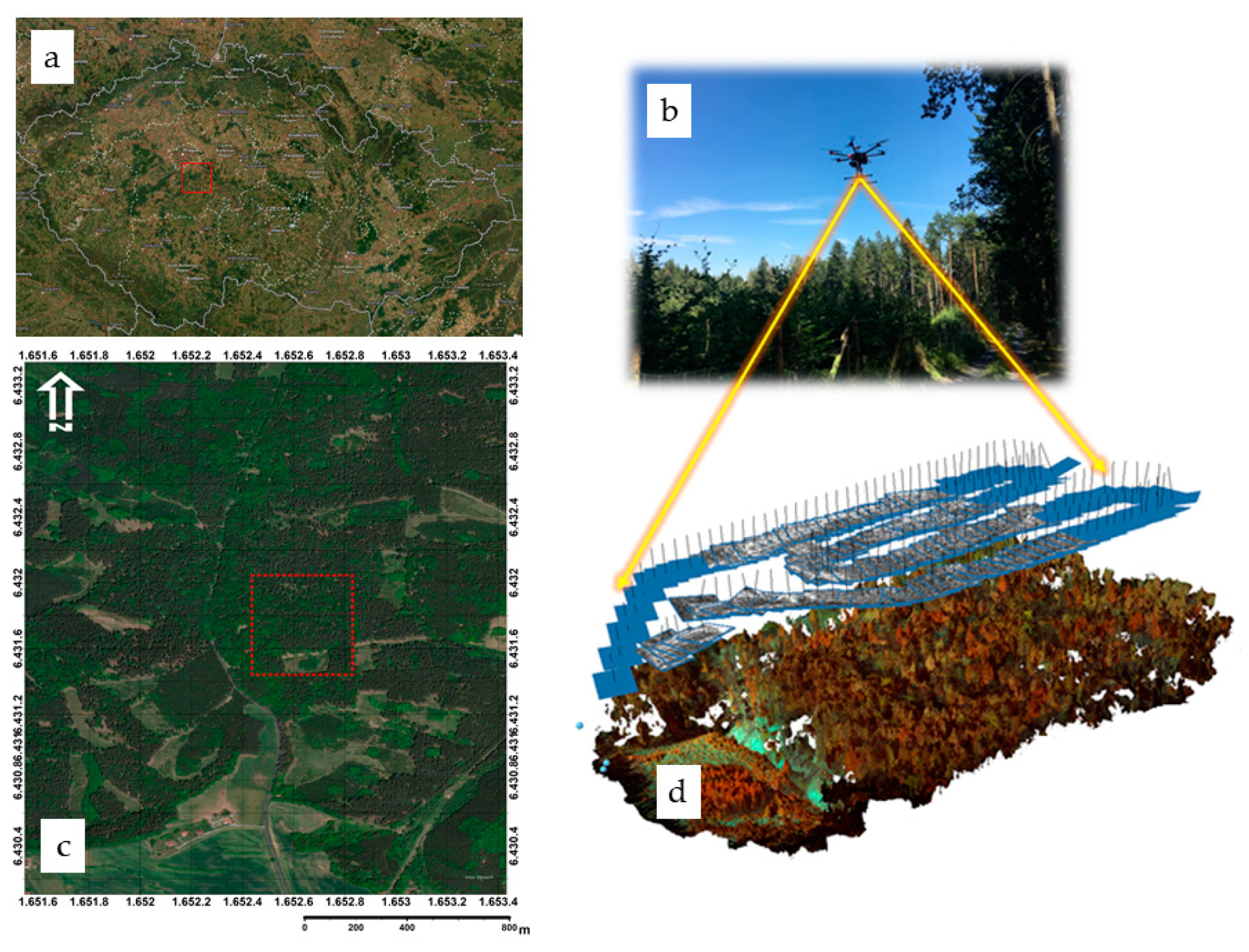
The forest site used in this study is located near the village of Oplany within the territory of the Training School Forest Enterprise in Kostelec, southeast of Prague, Czech Republic (Figure 1). The study area extends geographically from 49°55′6.25″ N; 14°50′34.84″ E to 49°54′56.34″ N, 14°50′54.26″ E. We established an experimental area of 180 × 160 m with an altitude of ~430 m a.s.l. and a mean annual temperature of 7.5 °C and mean annual precipitation of 600 mm. The study area is dominated by even-aged (originating from a clear-cut silvicultural treatment) coniferous tree species with an admixture of several broadleaf species, with a small percentage of understory (~20%). Norway spruce (Picea abies L.) and Scots pine (Pinus sylvestris L.) were the dominant conifer species, comprising 70% of all trees, accompanied mainly by Downy oak (Quercus pubescens Willd.), Hornbeam (Carpinus betulus L.), and Silver birch (Betula pendula Roth.), which comprised the remaining 30% of trees on the site. Norway spruce was the dominant species (75% of all conifers), and the three broadleaved species were equally represented. We eliminated all understory trees with a diameter at breast height (1.3 m; DBH) smaller than 15 cm from the field data. Field observations determined that there was evidence of increasing bark beetle outbreaks at alarming rates at the research site.
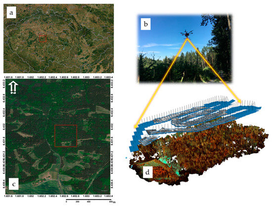
Figure 1.
(a) Shows the relative location of the study area in the Czech Republic (b) the used unmanned aerial system (UAS) DJI S900 embedded with the professional-grade multispectral camera MicaSense RedEdge-M (c) absolute location of the study area and (d) processed point cloud of the study area in false RGB image for spring 2019 and the applied flight path.
2.2. Reference Data
Field inventory and visual identification of tree species and health status assessments were conducted in August 2019. We assessed discoloration as a typical crown symptom, indicating the level of infestation which was caused by bark beetle infestation. Discoloration refers to any color anomalies occurring in live leaves [55]. Field-based species recognition and health status assessments (including bark visual analyses) were conducted by experienced forest experts in the study area by marking all the trees. Trimble M3 total station (Trimble Inc. Sunnyvale, CA, USA, 1978) was used to measure the tree positions. Initially, for evaluating the relation between reference data and predictor variables, all trees were classified according to tree type and health status into four classes: (i) healthy broadleaves = B, (ii) healthy conifers = C, (iii) infested conifers = I, and (iv) dead conifers = D (general classification). Afterward, depending on the health status and tree type, subgroups were created and the best independent variables were used for predicting the tree species and health status (detailed classification), using the SVM algorithm (Table 1) in STATISTICA V.12 (Dell Inc., Round Rock, TX, USA).

Table 1.
Classification summary table including both tree species and health status assessment from the reference data.
2.3. UAS Survey Planning and Data Collection
In total, two flights, conducted on 17 April and 24 July of 2019, were performed. Data from both flights were acquired between 11:00 a.m. and 14:00 p.m. local time under favorable weather conditions for photographing, were conducted using a rotary-wing DJI S900 (Dá-Jiāng Innovations Science and Technology Co. Ltd., Shenzhen, China) UAS equipped with a MicaSense RedEdge-M multispectral camera (MicaSense, Seattle, WA, USA); sensitive to the RGB, red-edge, and NIR spectral regions (Table 2). Since MicaSense RedEdge-M features global shutters it is less affected by normal vibration, gimbal was not a requirement in our study. Although we did not apply any interior calibration for the camera, the MicaSense calibrated reflectance panel (CRP) was used to convert raw pixel values into reflectance, using an image of CRP taken before and after the flight [56]. This was a necessary step during the processing phase in Metashape professional edition 64-bit V. 1.5.3.8469 (Agisoft LCC, St. Petersburg, Russia). The above mentioned procedure allows image pixel values to accurately describe the material composing the object of interest by compensating lighting and atmospheric conditions. Without the calibration process, data captured over different dates cannot be accurately compared for change detection. Furthermore, the copter was guided semi-automatically, with the route planned for a height of 110 m at a speed of 2 m·s−1 and capture rate of one image per second in all bands simultaneously, recording the position of each image using a high-performance GNSS receiver integrated into the DJI A2 flight control system of the DJI S900. According to the capture rate of the multispectral camera (1 image·s−1), flight planning resulted in 85% frontal overlapping and 70% side overlapping. DJI GO Version V. 4.1.9 was the program used for controlling the DJI S900. After approximately eight minutes of flight (based on the pre-defined flight parameters), manual control was regained and the copter was safely landed. For both flights, a single serpentine pattern was used with a nadir-pointing camera.

Table 2.
Spectral bands with center wavelength and bandwidth of the MicaSense RedEdge-M multispectral camera.
2.4. Photogrammetric Processing and Model Extraction
Multispectral aerial images from both periods were photogrammetrically processed using SfM in Metashape. To ensure optimal photo alignment results during the photogrammetric processing, the automatic image quality estimation feature in Metashape was considered to identify poorly focused images with a quality value of less than 0.5 units. The total number of images included in the alignment process for the first dataset (spring 2019) was 153 out of 153, while for the second dataset (summer 2019) 144 of 144 images taken were used. Feature extraction and matching were performed using the SIFT algorithm [18] to detect image feature points and match them between images. A bundle block adjustment was applied on the matched features between the images, to identify the XYZ location and camera orientation of each image feature resulted in a sparse 3D point cloud.
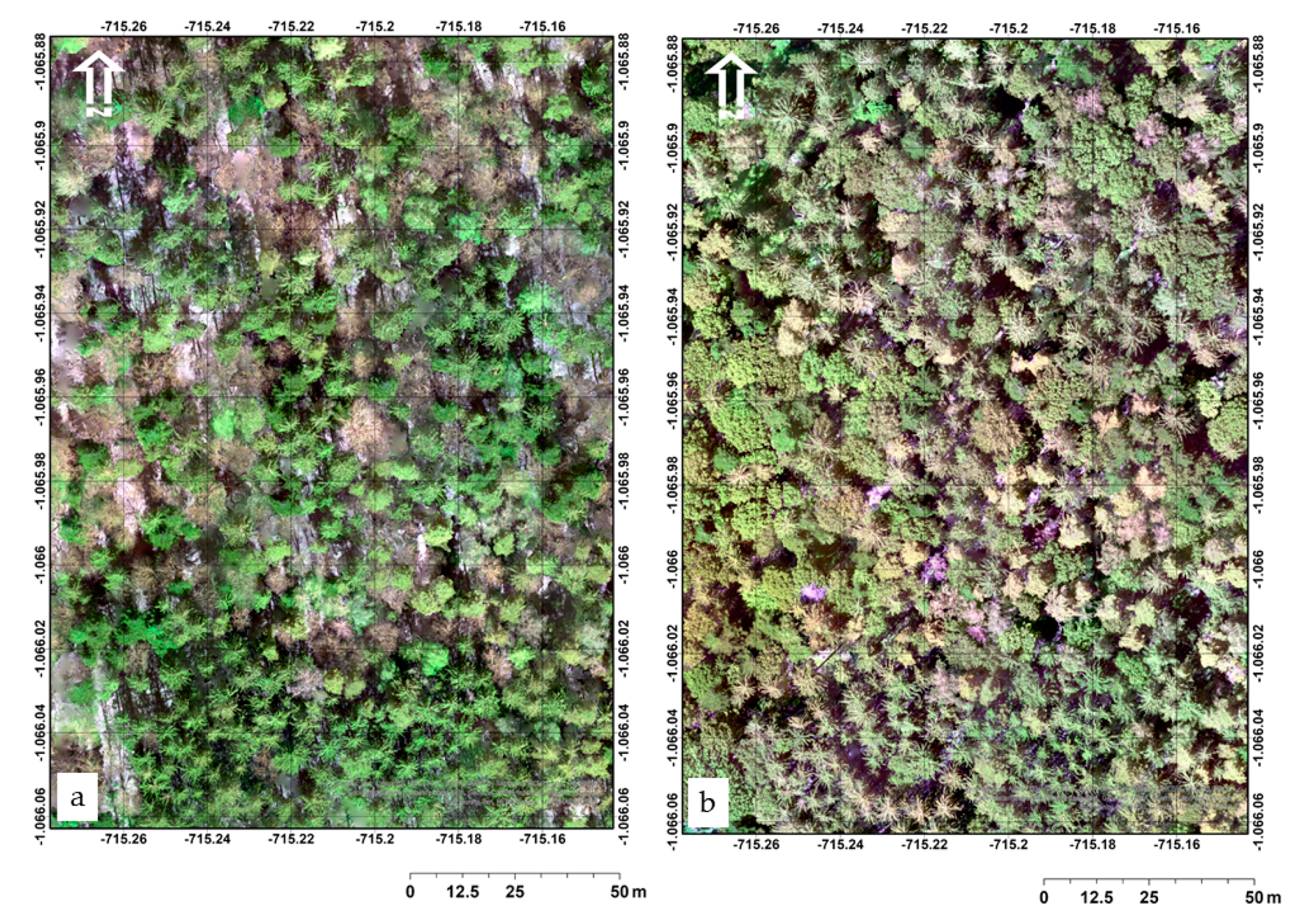
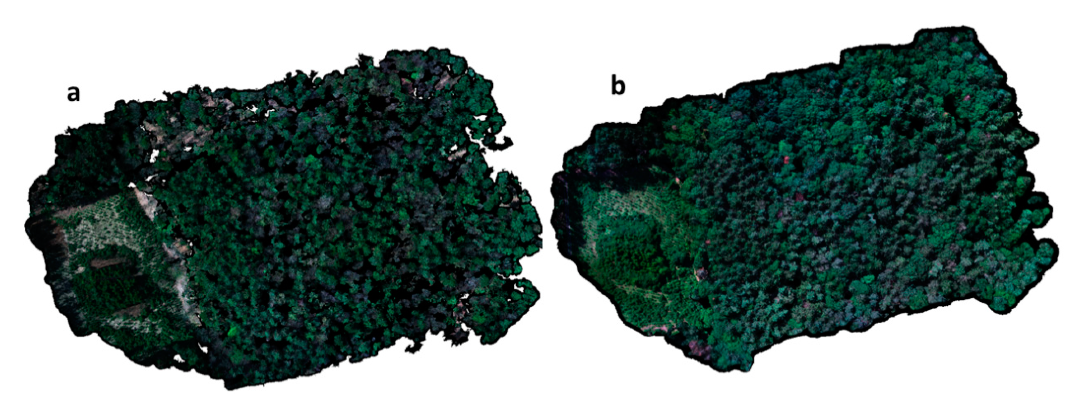
For photo alignment and dense point cloud generation, we chose ultra-high quality, resulting in little noise during the densification process, while for the depth filtering, the mild option was used. The ground points were then classified and mesh models were created from all point classes. The classification was automatic and it was based on three parameters: (a) maximum distance (m), (b) maximum angle (deg.) and (c) cell size. Texture was applied using the orthophotos for the mapping mode option. Digital terrain models (DTMs) were generated from the ground points and digital surface models (DSMs) were produced from the points of all classes for both datasets, with a resolution of 0.05 m. Additionally, orthophotos were exported for both datasets (Figure 2 and Figure 3). Before any process, we generated normalized canopy height models (nCHMs) by subtracting the DSM from the DTM in ArcMap 10.3.1 by ESRI©.
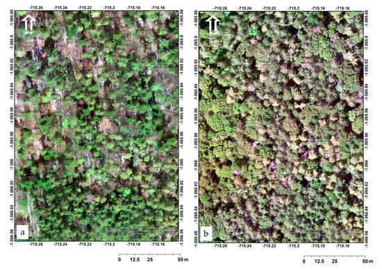
Figure 2.
Map perspective of the actual study area. (a) Shows the captured ortho-mosaic (RGB) of the study area by UAS at spring and (b) shows the captured ortho-mosaic (RGB) of the study area by UAS at summer.
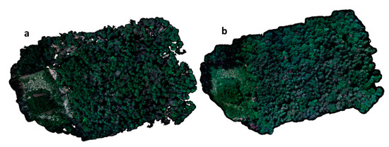
Figure 3.
Illustration of the resultant forest models. UAS orthophotos in RGB from both seasonal datasets; (a) spring 2019 and (b) summer 2019.
2.5. Spectral and Texture Analysis
Once the positions of all the trees in the study area were identified, a new point shapefile with the tree locations was created. To develop a deeper understanding of the spatial and temporal changes in the pattern (Figure 4) caused by seasonal changes (spring and summer 2019), several VIs including a variety of wavelength bands (RGB, red-edge, and NIR) were applied (Table 3) to evaluate the amount of vegetation cover change between the two seasons.
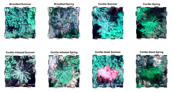
Figure 4.
Examples of zoomed tree canopies on different tree species and health status from both seasonal periods in RGB spectral bands.

Table 3.
Reflectance indices used in chronological order.
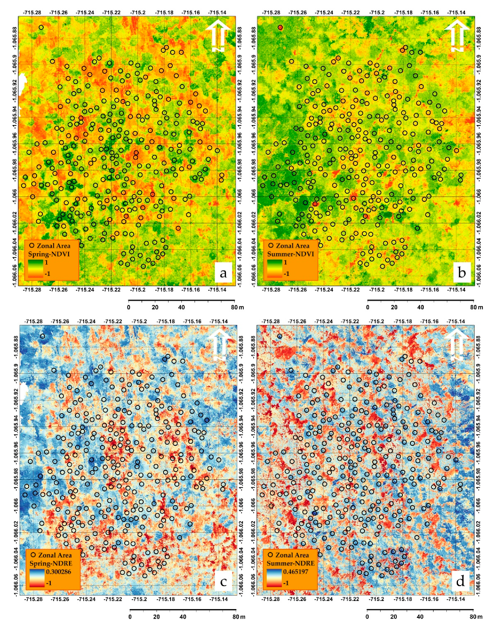
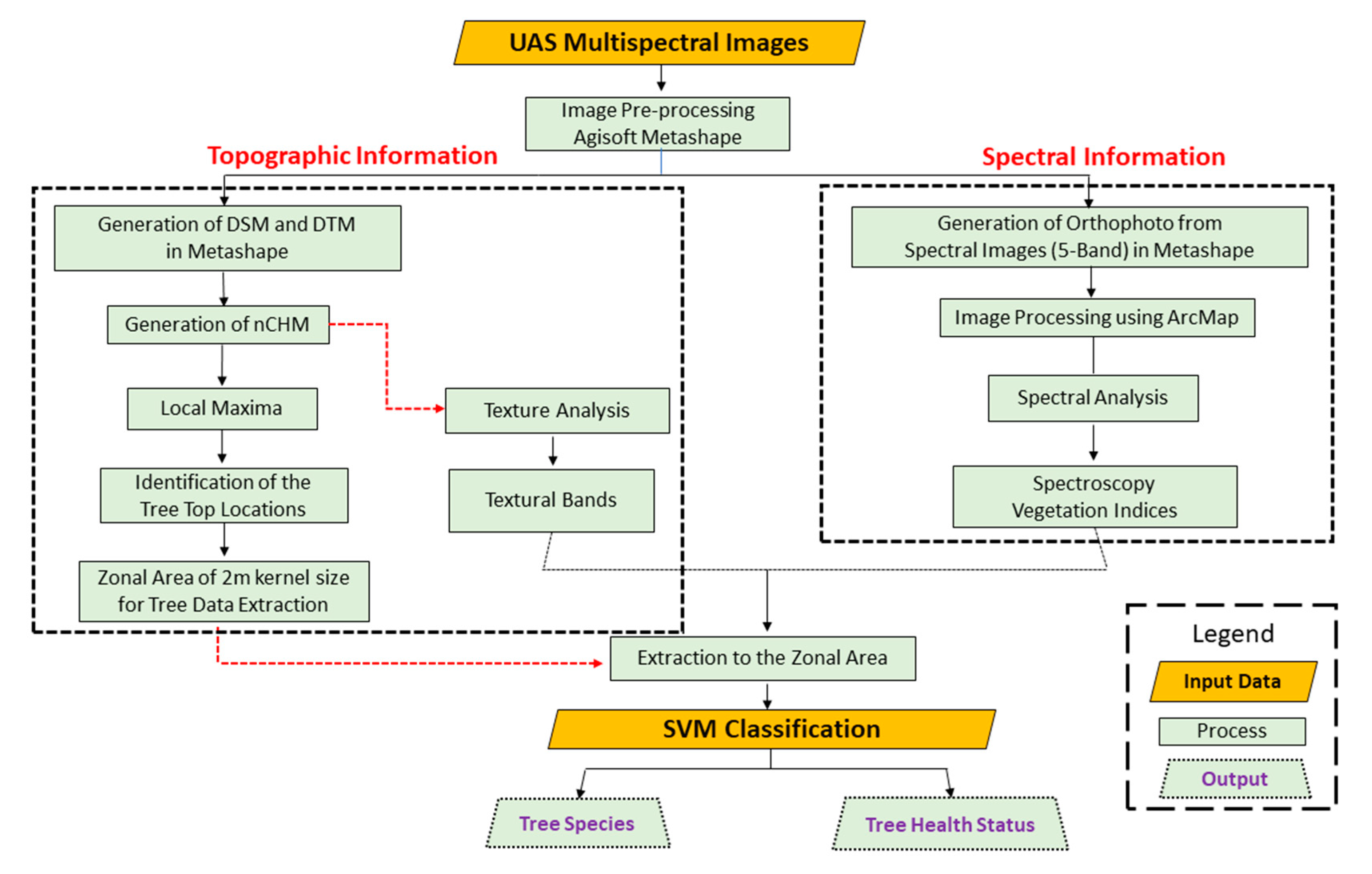
The PCI geomatica, version 2016.04.01 (PCI Geomatics, Markham, ON, Canada) was used to map the TA within the zonal areas from topographic information (nCHM). For each season, 13 nCHM-based TA layers were mapped, including Mean, Variance, Entropy, Contrast, Heterogeneity, Homogeneity, Angular Second Moment, Correlation, Gray-level Difference Vector (GLDV) Angular Second Moment, GLDV Entropy, GLDV Mean, GLDV Contrast, and Inverse Difference, with a kernel window size of 25 × 25 (32-bit). The main advantage of TA application on nCHMs is related to the fact that seasonal vegetation changes, as well as tree health status, can ultimately affect the structure of tree crown. For this reason, we assumed that the application of TA can lead to an optimum combined classification of forest tree species and health status assessment. A total of 26 TA layers were derived from nCHM for TA. Ultimately, to avoid overlapped tree crown areas and any uncertainties in the extracted values, a buffer zone with 2-m radius was used by means of zonal statistics in ArcMap (Figure 5). An overview of the methodology can be seen in Figure 6.
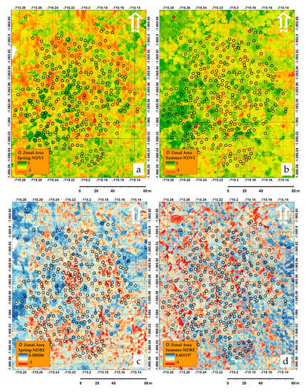
Figure 5.
(a) Showing the application of normalized difference vegetation index (NDVI) in spring (b) NDVI in summer (c) showing the normalized difference red-edge index (NDRE) in spring and (d) NDRE in summer (see details in Section 2.5).

Figure 6.
Flowchart of steps used for the classification of tree species and the detection of healthy, unhealthy (infested), and dead trees.
2.6. Classification Properties for the Distinguishment of Tree Species and Health Classes
In addition to the spectral and texture analysis that was applied for the general classification, the SVM algorithm was adopted for our unbalanced sample data in STATISTICA for conducting detailed classification (Table 1). For improving the accuracy of the output in our study, the SVM classifier type 1 was used. The training and validation samples were randomly selected as 70% for training and 30% for validation of the modeling in each category. For mapping not linearly separable classes, SVM has different kernel functions, among which the radial basis function (RBF) has shown superiority as to other functions [61,62]. RBF kernel was examined in a fixed number of gamma that was calculated according to 1/number of independent variables in SVM [46]. The adjustment of the gamma value influences the shape of the separating hyperplane and its value depends on the data interval and distribution and differs from one dataset to another [63,64]. For selecting the best parameters, V-fold cross-validation (V = 10) was used for minimizing the error function and improving the classification results. The general idea of using V-fold cross-validation is to divide the overall sample into several V-folds (randomly drawn disjoint sub-samples). The same type of SVM analysis is then successively applied to the observations belonging to the V-1 folds, and the results of the analyses are applied to sample V (the sample or fold that was not used to fit the SVM model) to compute the error, usually defined as the sum-of-squared. The results for the V replications are averaged to yield a single measure model error of the stability of the respective model, i.e., the validity of the model for predicting unseen data.
2.7. Statistical Analysis
We used SPSS Statistics V. 24 (IBM Corporation, Armonk, NY, U.S.A), STATISTICA V.12 (Dell Inc., Round Rock, TX, USA) and MATLAB® R2017b professional edition (MathWorks, MA, USA) for the statistical analysis and visualization of the collected data. Because our data were not normally distributed, Levene’s test was used to assess the equality of variances for all the tested statistical variables between the major classes; healthy broadleaves = B, healthy conifers = C, infested conifers = I, dead conifers = D for each VI. The following descriptive statistics were calculated for each VI and TA within each tree zonal area: Min, Max, Range, Mean, Standard deviation, Sum, Median, Variance, Mid-range, Skewness, and Kurtosis.
To determine the strength of the association between the categorical (independent) variable and numerical (dependent) variables, the Eta (η) coefficient was used (Equation (1)). Eta-squared (η2) was calculated to measure the coefficient of determination. Multiple comparisons were then applied to compare the means between the variables; the first one was Tuckey’s honest significance difference (HSD) test (Equation (2)), assuming equal variance, and the second was Dunnett’s T3 test. The latter does not assume any equality of variance for analyzing the differences between the groups (Equation (3)). A significance level (a) of 0.05 was used to determine whether or not the above tests were statistically significant.
where is the sum-of-squares between the groups and is the total sum-of-squares in the crosstab.
where − is the difference between the pair of means. To calculate this, should be larger than , is the mean square within, and is the number in the group or treatment.
where, refers to the critical value in the Dunnett critical value table, is mean square within groups, and n is the sample size.
Kappa index, overall accuracy, commission error and user’s accuracy used to evaluate the accuracy of SVM predicted results, given by Equations (4)–(7).
where is the observed agreement and is the expected agreement by chance.
where OA stands for overall accuracy, stands for correctly predicted values, and is the total number of test data.
where CE stands for commission error, stands for incorrect predicted values and is the number of trees predicted by SVM (correct or not correct) for each class, UA stands for user’s accuracy.
However, according to the study by Shao et al. [65], the use of Kappa is associated with a series of theoretical flaws-uncertainties for accuracy assessment. Thus, for supporting the effectiveness of our methodology the F-score [66], omission error (OE), and producer’s accuracy (PA) were calculated using Equations (8)–(10).
where OE stands for omission error, IP stands for incorrect predicted values and NO is the number of observed trees for each class, PA is the producer’s accuracy.
3. Results and Discussion
3.1. Spectral Analysis
The results of the multiple comparisons for both seasons showed that there was a significant difference in the amount of VIs between the major classes. As we assumed due to unbalanced reference data, Levene’s test revealed that there was heterogeneity of variances between the classes for the majority of VI classification cases, as described in Table S1.
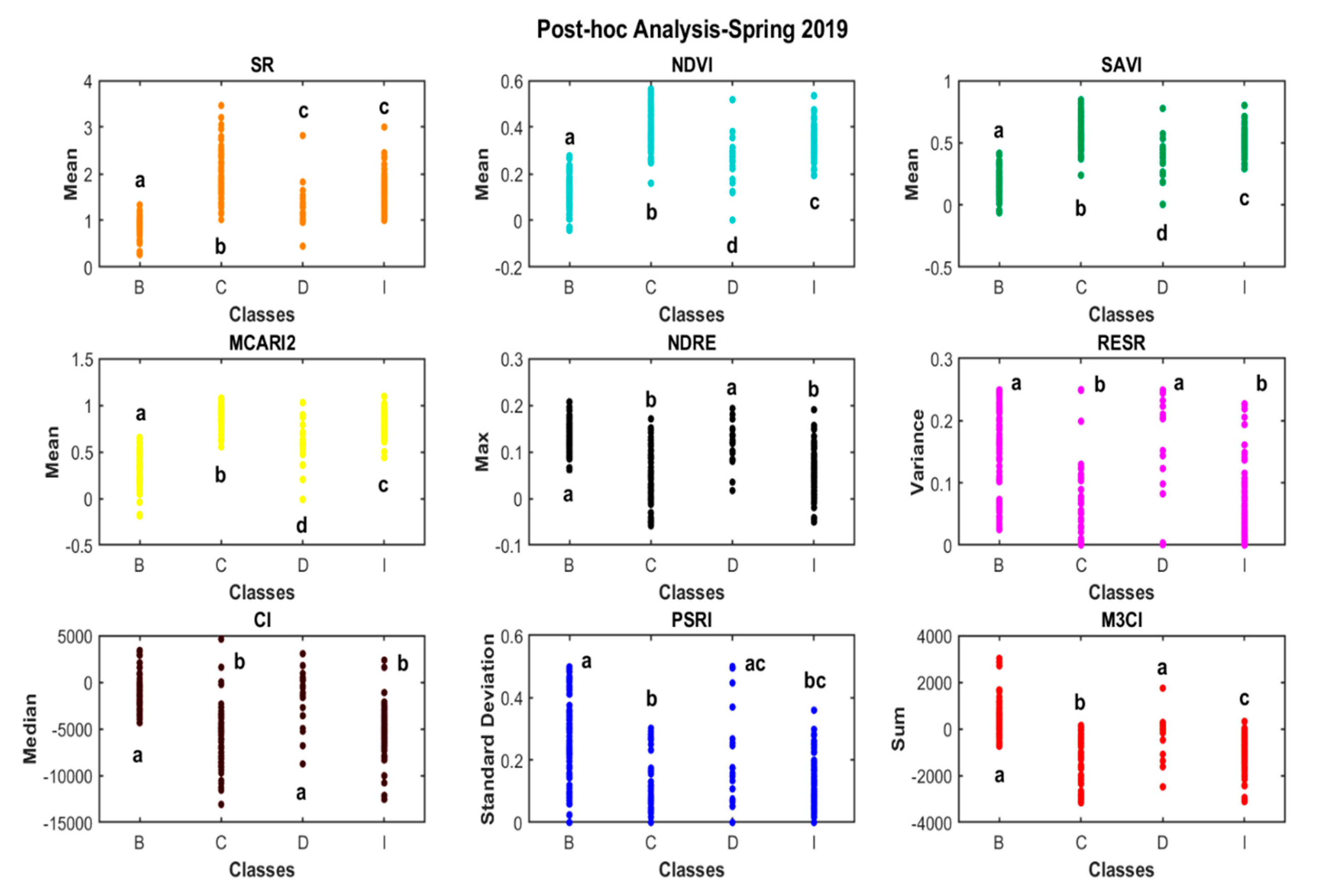
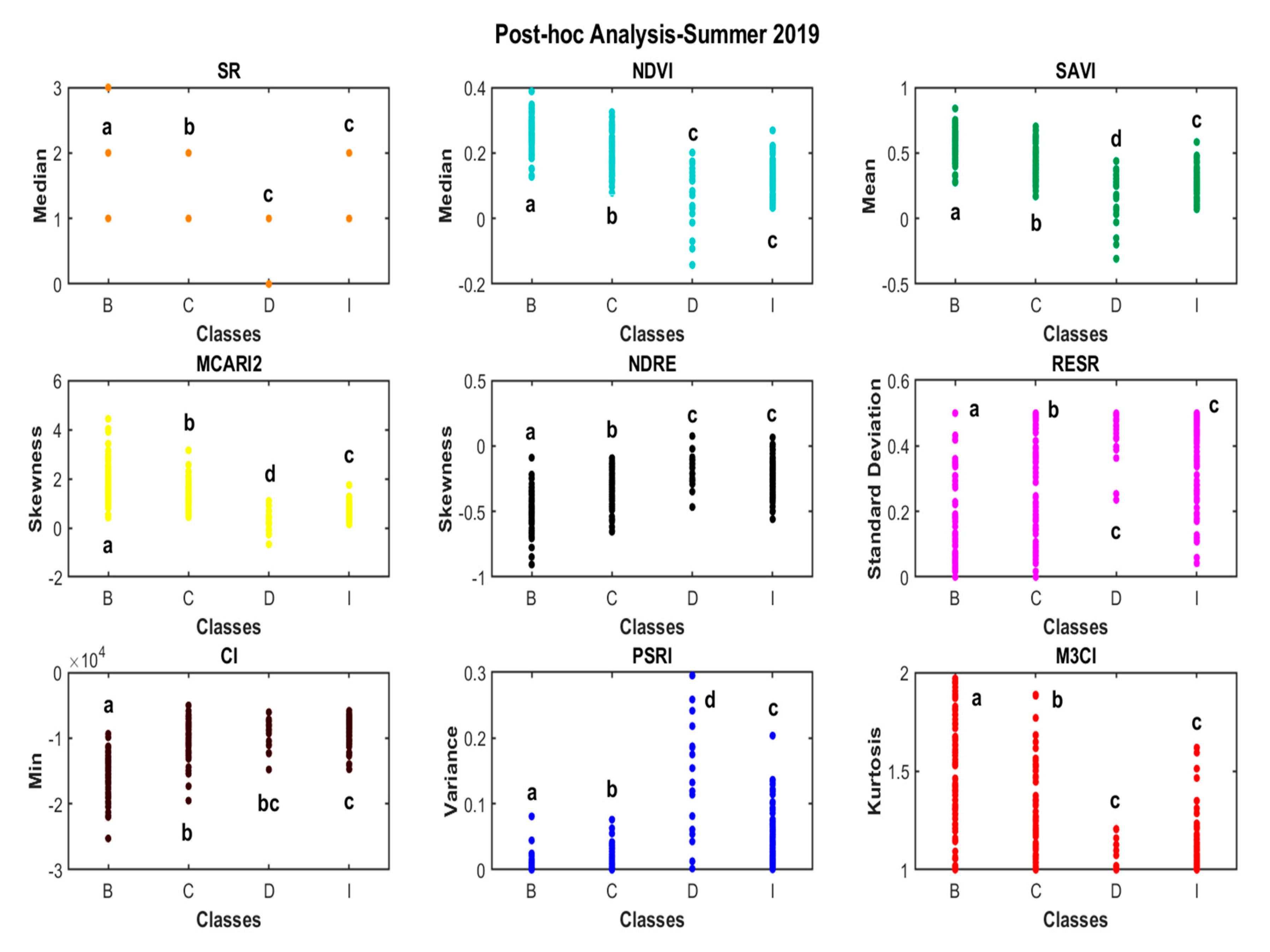
It is obvious from the post-hoc analysis in Figure 7 that NDVI, SAVI, and MCARI2 performed the best in classifying the reference data from spring 2019, whereas SAVI, MCARI2, and PSRI had the best performance for the summer period (Figure 8). The above-mentioned VIs were able to successfully distinguish all the major classes from each other. Since the mentioned VIs are based on NIR, red, and red-edge wavelengths, they can detect the changes occurring in the amount of chlorophyll absorption and reflectance of the cellular structure of the leaves [67,68,69]. When the tree is dehydrated or afflicted with a disease, spongy layers within the leaf surface deteriorate, thus, a tree absorbs more NIR compared to a healthy tree [29,30,31].
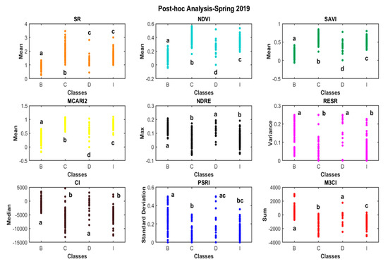
Figure 7.
Post-hoc analysis for vegetation indices (VIs) showing the strength of association between the four major categorical classes (healthy broadleaves = B, healthy conifers = C, infested conifers = I, dead conifers = D) and the most significant descriptive statistics for each VI. Small letters (a–d) were used to denote significant differences between groups (p-value < 0.05).
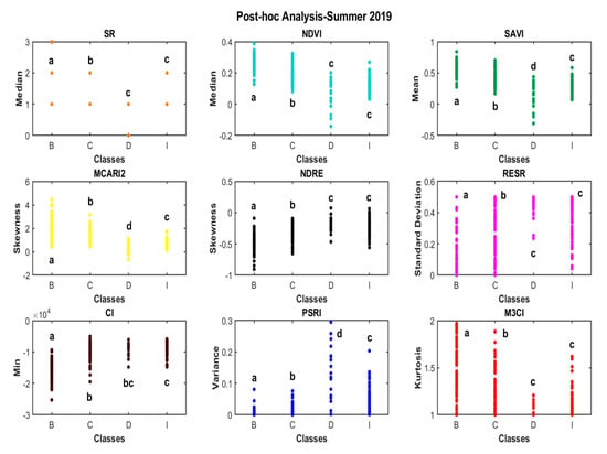
Figure 8.
Post-hoc analyses for vegetation indices (VIs) showing the strength of association between the four major categorical classes (healthy broadleaves = B, healthy conifers = C, infested conifers = I, dead conifers = D) and the most significant descriptive statistics for each VI. Small letters (a–d) were used to denote significant differences between groups (p-value < 0.05).
The post-hoc results highlighted an issue for the differentiation between major classes in spring between healthy broadleaves (B) and dead conifers (D), which likely occurred because of the nature of broadleaves being without leaves during the spring. This issue resulted in confusion in the identification of major classes in the case of RESR, M3CI, CI, PSRI, and NDRE VI layers.
According to the coefficient of determination Eta-squared (η2), MCARI2 and CI respectively had the highest correlation with field data major classes with Eta-squared (η2) of 0.73 in spring 2019 and 0.61 for summer 2019, as described in Table S2. These results confirm the importance of the red-edge band in tree type and health status assessment. Post-hoc results for the summer exhibited better performance of PSRI compared to NDVI in the classification of reference data in different major classes. The results of Eta-squared (η2) were used to select the best independent variables, including VI and TA, for further analysis with the SVM.
3.2. Texture Analysis
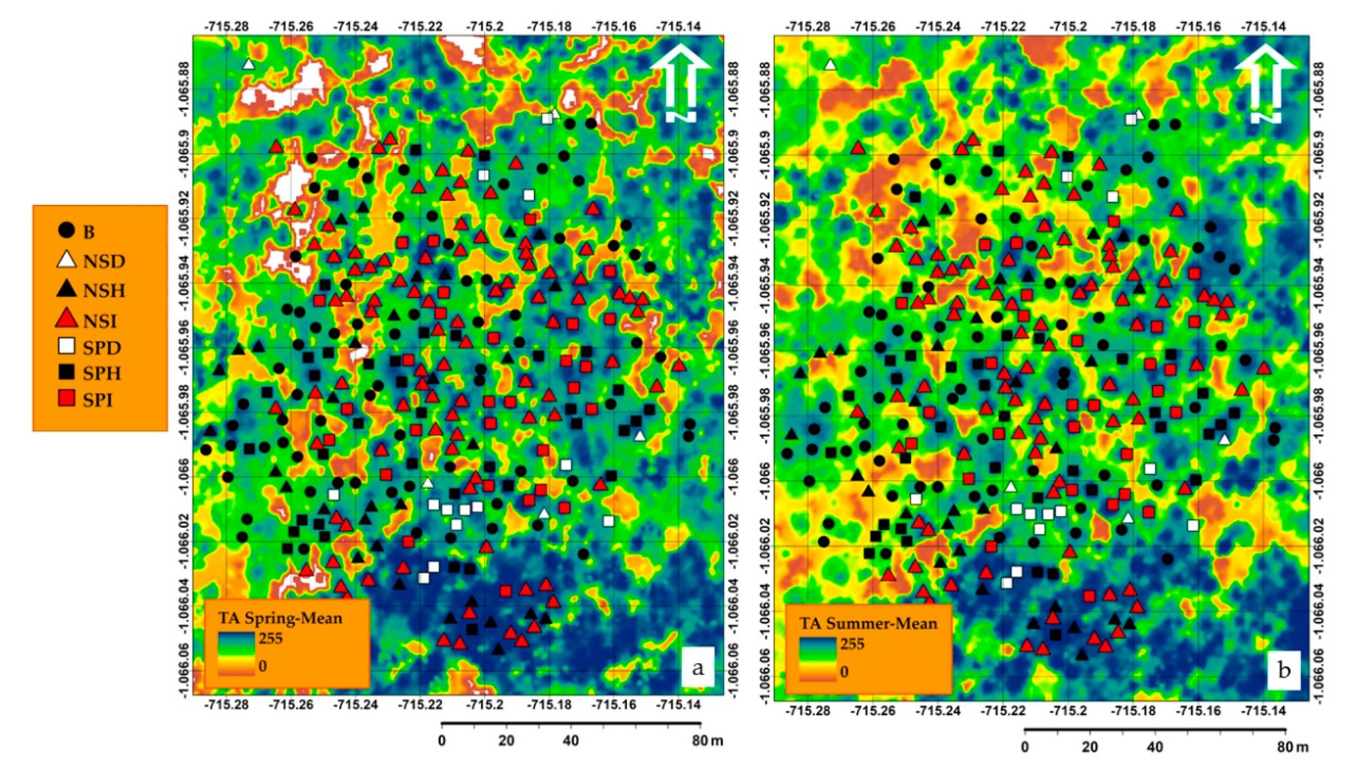
Similar to the spectral analysis, multiple comparisons result for TA revealed that there was a significant difference in the amount of nCHM-based texture values between the major classes. Due to the unbalanced reference data, Levene‘s test demonstrated that there was heterogeneity of variances between the classes for the majority of texture values (Table S1). Eta-squared (η2) exhibited that in most cases there was a weak or moderate relationship between predicted and observed values (e.g., Dissimilarity = 0.14, GLDV Angular Second Moment = 0.22, GLDV Entropy = 0.22, GLDV Mean = 0.14, Inverse Difference = 0.15, and Standard Deviation = 0.17), as described in Table S3. nCHM-based Mean was the only variable that showed a stronger relationship with the reference data compared to the rest of variables (Figure 9 and Figure 10), with an Eta-squared (η2) of 0.51 in spring 2019 and 0.28 for summer 2019, as described in Table S3.
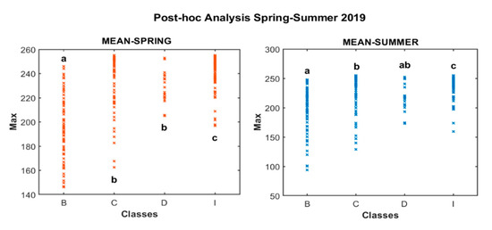
Figure 9.
Post-hoc analysis for texture analysis (TA) showing the strength of association between the four major categorical classes (healthy broadleaves = B, healthy conifers = C, infested conifers = I, dead conifers = D) and the most significant descriptive statistic derived for the Mean variable in both seasons. Small letters (a–d) were used to denote significant differences between the groups (p–value < 0.05).
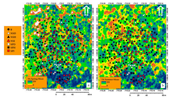
Figure 10.
Mean texture measure parameter applied in the normalized canopy height model (nCHM) (a) in spring and (b) in summer, including the locations of healthy, infested, and dead trees based on their species classes (B = Broadleaves, NSD = Norway spruce dead, NSH = Norway spruce healthy, NSI = Norway spruce infested, SPD = Scots pine dead, SPH = Scots pine healthy, SPI = Scots pine infested).
3.3. Detailed Tree Species Classification and Health Status Assessment by SVM
Based on Eta-squared (η2) results, all the VI layers which had strong relation with the reference data were used for modeling process using SVM. Those layers are: CI (Min) summer, CI (Median) spring; M3CI (Sum) spring, M3CI (Kurtosis) summer; MCARI (Mean) spring, MCARI (Skewness) summer; NDRE (Maximum) spring, NDRE (Skewness) summer; NDVI (Mean) spring, NDVI (Median) summer; PSRE (STD) spring, PSRE (Variance) summer; RESR (Variance) spring, RESR (STD) summer; SR (Mean) spring, SR (Median) summer; SAVI (Mean) spring, SAVI (Mean) summer (Table 4). Modeling tree species using the above layers successfully distinguished the reference data into detailed classes, producing an F–score of 95.65% for broadleaves, 78.48% for Norway spruce and 53.75% for Scots pine, resulting in OA of 78.82% (Table 4). This result confirms similar UAS-based studies on tree species multispectral classification accuracies reported elsewhere [22,23,24,70]. To improve the model accuracy, fusion of the TA and VI layers was used for modeling the reference data. The criteria for the selection of TA layers for SVM were exclusively based on Eta-squared (η2) results. For TA layers we chose layers with moderate and strong relationship with the reference data, such as Mean (Mean) spring/summer; STD (Range) summer; GLDV Angular Second Moment (Skewness) summer; GLDV Entropy (Range) summer; GLDV Angular Second Moment (Coefficient of Variation) summer.

Table 4.
Tree species classification summary table and confusion matrix using selected VI layers.
The combination of VI and TA layers successfully improved accuracy of modeling tree species using SVM by 2.36% (OA) (Table 5). SVM was able to successfully separate broadleaves from the rest of the classes with an accuracy of 100%, resulting in both CE and OE of 0%. Similarly, SVM exhibited the ability to distinguish the Norway spruce from broadleaves and Scots pine trees with PA of 91.89%, resulting in an OE of 8.11%. Consequently, the OA for distinguishing reference data for tree species from SVM was 81.18%. Our method reliably distinguished between broadleaved and coniferous trees (Table 5). We estimated a Kappa of 0.70, which suggested a strong (substantial) relationship between the reference data and the independent variables. In addition, the combination of selected layers improved the amount of F-score values of 100% for broadleaves, 80.95% for Norway spruce, and 61.90% for Scots pine, respectively.

Table 5.
Tree species classification summary table and confusion matrix derived from the support vector machine (SVM) analysis using a combination of VI and TA layers.
Considering only tree health status, combination of TA and VI layers could not improve the accuracy of health status classification. However, using solely VI layers the SVM algorithm distinguished the classes with a very high OA of 84.71% (Table 6). The result is similar with the result of Näsi et al. [12]. Moreover, the results from CE in all cases validate the significance of our proposed methodology for the classification of the reference data into reliable classes. More specifically, the PA for all tree health classes was found to be ≥80%. Similar to the tree species classification, the Kappa for the assessment of health status was 0.66, which also suggested a substantial relationship between the reference data and the independent variables. In addition, F-score values for broadleaves, Norway spruce, and Scots pine were 72.73%, 88.64%, 81.69%, respectively.

Table 6.
Classification summary table and confusion matrix of tree health status derived from the support vector machine (SVM) using VI layers.
Classification of tree species/health using the selected VI layers successfully distinguished the reference data into detailed classes, producing an OA of 65.17% (Table 7).

Table 7.
Classification summary table and confusion matrix including combined tree species and health status derived from the support vector machine (SVM) analysis using VI layers.
The SVM analysis showed significant performance for dividing the reference data into more complex classes that contained tree species and health status simultaneously. Although SVM analysis showed significant performance for dividing the reference data to a more complex classes, it could not distinguish the different species among the dead trees (Table 7). Our results showed that SVM characteristics such as (a) a high generalization ability and acquisition of high modeling accuracies, (b) convexity of the cost function, (c) powerful in the treatment of high-dimensional data (e.g., hyperspectral data), and (d) limited effort required for architecture design and training step compared to other machine learning algorithms make SVM one of the most powerful non-parametric algorithm that can be significantly helpful for modeling complex sets of data derived from complex environments such as forests [61,62,63,64].
As evident in Table 8, combination of TA and VI layers showed an increase in OA by 4.24%. NSI and SPD classes were successfully distinguished with very high PA, 92% and 100%, respectively, which resulted in an OA of 69.41%. The proposed methodology for classifying SPH yielded poorer, yet comparable, performance when compared to the NSI and SPD. It is evident in Table 8 that a lack of sufficient reference data [71] in some of the classes (e.g., NSD) caused poor performance in the classification process using the SVM classifier. When combining tree species and health status, as expected, the Kappa was poorer yet comparable (0.59), which represented a moderate relationship between reference data and independent variables. As a result of data combination between texture and VI, we were able to improve significantly the distinguishment of coniferous species between healthy trees. The amount of F-score increased by 12.5% for healthy Norway spruce and 6.8% for the healthy Scots pine. Once more this result confirms that non-parametric algorithms such as SVM can be used as a powerful tool for modeling complex environments when a combination of unlimited thematic, spectral, and topographic layers are required [72]. Moreover, based on the result from Table 7 and Table 8, the distinguishment of tree species among the dead trees (coniferous) was not possible because of the similarity of reflectance of the dead leaves.

Table 8.
Classification summary table and confusion matrix including combined tree species and health status derived from the support vector machine (SVM) analysis using a combination of VI and TA layers.
4. Conclusions
Our primary interest was to investigate the capability of low-cost UAS-based bi-temporal multispectral photogrammetry using the MicaSense RedEdge-M sensor to detect and distinguish tree species and evaluate their health status in mixed forest conditions. Due to the ability of UAS to acquire data in ultra-high spatial and temporal resolutions, our method not only enabled mapping of the tree species and its current health state, but it also aids in monitoring the spread of disease, designating the possibility of either early-stage detection or new disease outbreaks to adjacent healthy trees. This would support precision forest management and local decision-making.
Based on a combination of a bi-temporal integrated spectral and texture information as well as supervised machine learning techniques, we aimed to extract the reflectance values within a buffer zone of 2-m radius from each treetop and not to map the canopy extent of each tree. Using the same buffer zone, we eliminated the impact of crown shape and vague pixels from the overlapped crown areas. The results indicated that the proposed methodology delivered satisfactory outputs and achieved sufficiently accurate and reliable tree species classification with an OA of 81.18%, and a health status assessment with an OA of 84.70%. Chlorophyll index red-edge (CI) had the highest correlation with field data major classes with Eta-squared (η2) of 0.61 compared to the rest of vegetation indices for summer 2019. That confirms the importance of the red-edge band for detail classification of both tree species type and health status during the vegetation period, due to the sensitivity of the red-edge band to small variations in the chlorophyll content and consistent across most species and health status classes.
This study confirmed the high efficiency of SVM with limited and unbalanced training samples and it allows users to combine an unlimited amount of different types of data (e.g., categorical and continuous input layers). Consequently, the combination of VI and TA layers for combined tree species and health status increased the OA by 4.24%. Conclusively, this approach can provide a new dimension of information derived from UAS platforms, which can lead to a better understanding of health status and tree species composition with reliable accuracy. Moreover, the results revealed that textural parameters of healthy tree crowns can be of significant importance in tree species classification. Distinguishment of species between dead trees could not be achieved due to the similar reflectance. This fact might be associated with the amount of error found in tree species classification between conifers, possibly due to the inability of the SVM algorithm to assign the dead conifer trees to one of the two coniferous classes. That is why higher accuracy has been found in broadleaves compared to the coniferous classes.
Limitations in the sampling from certain classes by multispectral sensors account for any of the uncertainties associated with our proposed approach. Identification of physiological stress in earlier stages or detection of smaller spectral differences could be possible with higher reliability and accuracy using hyperspectral sensors in wavelengths that cannot be covered by multispectral sensors. We also strongly believe that the use of thermal sensors could improve the classification of different tree species and health status. Nevertheless, UAS paired with multispectral sensors can significantly reduce the operational costs of monitoring forested areas on small to medium scales.
Supplementary Materials
The following are available online at https://www.mdpi.com/2072-4292/12/22/3722/s1, Table S1: Test of homogeneity of variance. Table S2: Eta results-Spectral analysis. Table S3: Eta results-Texture analysis.
Author Contributions
A.A. conceived the idea for this manuscript; D.P. and A.A. designed and wrote the manuscript; A.A. processed the remote sensing and terrestrial data. D.P. and A.A. designed and performed the statistical analyses; D.P. and A.A. finalized the manuscript. All authors have read and agreed to the published version of the manuscript.
Funding
This study was financially supported by EVA4.0 “Advanced Research Supporting the Forestry and Wood-processing Sector’s Adaptation to Global Change and the 4th Industrial Evolution” (No. CZ.02.1.01/0.0/0.0/16_019/0000803) of the Faculty of Forestry and Wood Sciences (FFWS) from the Czech University of Life Sciences (CULS) in Prague.
Acknowledgments
We acknowledge that this study was supported by EVA4.0 “Advanced Research Supporting the Forestry and Wood-processing Sector’s Adaptation to Global Change and the 4th Industrial Evolution ” (No. CZ.02.1.01/0.0/0.0/16_019/0000803) of the Faculty of Forestry and Wood Sciences (FFWS) from the Czech University of Life Sciences (CULS) in Prague. We would like to thank Peter Surový from the department of Forest Management of the Faculty of Forestry and Wood Sciences (FFWS) from the Czech University of Life Sciences (CULS) in Prague for his contribution to the collection of UAS data.
Conflicts of Interest
The authors declare no conflict of interest.
References
- Battisti, A.; Stastny, M.; Netherer, S.; Robinet, C.; Schopf, A.; Roques, A.; Larsson, S. Expansion of geographic range in the pine processionary moth caused by increased winter temperatures. Ecol. Appl. 2005, 15, 2084–2096. [Google Scholar] [CrossRef]
- Björkman, C.; Bylund, H.; Klapwijk, M.J.; Kollberg, I.; Schroeder, M. Insect Pests in Future Forests: More Severe Problems? Forests 2011, 2, 474–485. [Google Scholar] [CrossRef]
- Kurz, W.A.; Dymond, C.C.; Stinson, G.; Rampley, G.J.; Neilson, E.T.; Carroll, A.L.; Ebata, T.; Safranyik, L. Mountain pine beetle and forest carbon feedback to climate change. Nature 2008, 452, 987–990. [Google Scholar] [CrossRef] [PubMed]
- Nabuurs, G.-J.; Lindner, M.; Verkerk, P.J.; Gunia, K.; Deda, P.; Michalak, R.; Grassi, G. First signs of carbon sink saturation in European forest biomass. Nat. Clim. Chang. 2013, 3, 792–796. [Google Scholar] [CrossRef]
- Seidl, R.; Thom, D.; Kautz, M.; Martin-Benito, D.; Peltoniemi, M.; Vacchiano, G.; Wild, J.; Ascoli, D.; Petr, M.; Honkaniemi, M.P.J.; et al. Forest disturbances under climate change. Nat. Clim. Chang. 2017, 7, 395–402. [Google Scholar] [CrossRef]
- Álvarez-Taboada, F.; Paredes, C.; Julián-Pelaz, J. Mapping of the Invasive Species Hakea sericea Using Unmanned Aerial Vehicle (UAV) and WorldView-2 Imagery and an Object-Oriented Approach. Remote Sens. 2017, 9, 913. [Google Scholar] [CrossRef]
- Fassnacht, F.E.; Latifi, H.; Stereńczak, K.; Modzelewska, A.; Lefsky, M.; Waser, L.T.; Straub, C.; Ghosh, A. Review of studies on tree species classification from remotely sensed data. Remote Sens. Environ. 2016, 186, 64–87. [Google Scholar] [CrossRef]
- Hynynen, J.; Ahtikoski, A.; Siitonen, J.; Sievänen, R.; Liski, J. Applying the MOTTI simulator to analyse the effects of alternative management schedules on timber and non-timber production. For. Ecol. Manag. 2005, 207, 5–18. [Google Scholar] [CrossRef]
- Repola, J. Biomass equations for Scots pine and Norway spruce in Finland. Silva. Fenn. 2009, 43, 625–647. [Google Scholar] [CrossRef]
- Panagiotidis, D.; Abdollahnejad, A.; Surový, P.; Chiteculo, V. Determining tree height and crown diameter from high-resolution UAV imagery. Int. J. Remote Sens. 2017, 38, 2392–2410. [Google Scholar] [CrossRef]
- Abdollahnejad, A.; Panagiotidis, D.; Surový, P. Estimation and Extrapolation of Tree Parameters Using Spectral Correlation between UAV and Pléiades Data. Forests 2018, 9, 85. [Google Scholar] [CrossRef]
- Näsi, R.; Honkavaara, E.; Lyytikäinen-Saarenmaa, P.; Blomqvist, M.; Litkey, P.; Hakala, T.; Viljanen, N.; Kantola, T.; Tanhuanpää, T.; Holopainen, M. Using UAV-Based Photogrammetry and Hyperspectral Imaging for Mapping Bark Beetle Damage at Tree-Level. Remote Sens. 2015, 7, 15467–15493. [Google Scholar] [CrossRef]
- Moriya, E.A.S.; Imai, N.N.; Tommaselli, A.M.G.; Miyoshi, G.T. Mapping Mosaic Virus in Sugarcane Based on Hyperspectral Images. IEEE J. Sel. Top. Appl. Earth Obs. Remote Sens. 2016, 10, 740–748. [Google Scholar] [CrossRef]
- Onishi, M.; Ise, T. Automatic classification of trees using a UAV onboard camera and deep learning. arXiv 2018, arXiv:1804.10390. [Google Scholar]
- Ørka, H.O.; Næsset, E.; Bollandsås, O.M. Classifying species of individual trees by intensity and structure features derived from airborne laser scanner data. Remote Sens. Environ. 2009, 113, 1163–1174. [Google Scholar] [CrossRef]
- Snavely, N.; Seitz, S.M.; Szeliski, R. Modeling the World from Internet Photo Collections. Int. J. Comput. Vis. 2008, 80, 189–210. [Google Scholar] [CrossRef]
- Koenderink, J.J.; Van Doorn, A.J. Affine structure from motion. J. Opt. Soc. Am. A 1991, 8, 377–385. [Google Scholar] [CrossRef] [PubMed]
- Cruz-Mota, J.; Bogdanova, I.; Paquier, B.; Bierlaire, M.; Thiran, J.-P. Scale Invariant Feature Transform on the Sphere: Theory and Applications. Int. J. Comput. Vis. 2012, 98, 217–241. [Google Scholar] [CrossRef]
- Fonstad, M.A.; Dietrich, J.T.; Courville, B.C.; Jensen, J.L.; Carbonneau, P.E. Topographic structure from motion: A new development in photogrammetric measurement. Earth Surf. Process. Landf. 2013, 38, 421–430. [Google Scholar] [CrossRef]
- Micheletti, N.; Chandler, J.H.; Lane, S.N. Structure from Motion (SFM) Photogrammetry. In Geomorphological Techniques; Clarke, L.E., Nield, J.M., Eds.; British Society for Geomorphology: London, UK, 2015; Chapter 2; pp. 1–12. [Google Scholar]
- Coburn, C.; Roberts, A.C.B. A multiscale texture analysis procedure for improved forest stand classification. Int. J. Remote Sens. 2004, 25, 4287–4308. [Google Scholar] [CrossRef]
- Lisein, J.; Michez, A.; Claessens, H.; Lejeune, P. Discrimination of Deciduous Tree Species from Time Series of Unmanned Aerial System Imagery. PLoS ONE 2015, 10, e0141006. [Google Scholar] [CrossRef] [PubMed]
- Franklin, S.E.; Ahmed, O.S.; Williams, G. Northern Conifer Forest Species Classification Using Multispectral Data Acquired from an Unmanned Aerial Vehicle. Photogramm. Eng. Remote Sens. 2017, 7, 501–507. [Google Scholar] [CrossRef]
- Gini, R.; Sona, G.; Ronchetti, G.; Passoni, D.; Pinto, L. Improving Tree Species Classification Using UAS Multispectral Images and Texture Measures. ISPRS Int. J. Geo-Inf. 2018, 7, 315. [Google Scholar] [CrossRef]
- Feng, Q.; Liu, J.; Gong, J. UAV Remote Sensing for Urban Vegetation Mapping Using Random Forest and Texture Analysis. Remote Sens. 2015, 7, 1074–1094. [Google Scholar] [CrossRef]
- Kelcey, J.; Lucieer, A. An adaptive texture selection framework for ultra-high resolution UAV imagery. In Proceedings of the 2013 IEEE International Geoscience and Remote Sensing Symposium–IGARSS, Melbourne, VIC, Australia, 21–26 July 2013; Institute of Electrical and Electronics Engineers (IEEE): New York, NY, USA, 2013; pp. 3883–3886. [Google Scholar] [CrossRef]
- Senf, C.; Seidl, R.; Hostert, P. Remote sensing of forest insect disturbances: Current state and future directions. Int. J. Appl. Earth Obs. Geoinf. 2017, 60, 49–60. [Google Scholar] [CrossRef]
- Klouček, T.; Komárek, J.; Surový, P.; Hrach, K.; Janata, P.; Vašíček, B. The Use of UAV Mounted Sensors for Precise Detection of Bark Beetle Infestation. Remote Sens. 2019, 11, 1561. [Google Scholar] [CrossRef]
- Dash, J.; Curran, P.J. The MERIS terrestrial chlorophyll index. Int. J. Remote Sens. 2004, 25, 5403–5413. [Google Scholar] [CrossRef]
- Clevers, J.; Gitelson, A. Remote estimation of crop and grass chlorophyll and nitrogen content using red-edge bands on Sentinel-2 and -3. Int. J. Appl. Earth Obs. Geoinf. 2013, 23, 344–351. [Google Scholar] [CrossRef]
- Clevers, J.G.P.W.; Kooistra, L. Using Hyperspectral Remote Sensing Data for Retrieving Canopy Chlorophyll and Nitrogen Content. IEEE J. Sel. Top. Appl. Earth Obs. Remote Sens. 2011, 5, 574–583. [Google Scholar] [CrossRef]
- Merzlyak, M.N.; Gitelson, A.A.; Chivkunova, O.B.; Rakitin, V.Y. Non-destructive optical detection of pigment changes during leaf senescence and fruit ripening. Physiol. Plant. 1999, 106, 135–141. [Google Scholar] [CrossRef]
- Rautiainen, M.; Mõttus, M.; Heiskanen, J.; Akujärvi, A.; Majasalmi, T.; Stenberg, P. Seasonal reflectance dynamics of common understory types in a northern European boreal forest. Remote Sens. Environ. 2011, 115, 3020–3028. [Google Scholar] [CrossRef]
- Cole, B.; McMorrow, J.; Evans, M. Spectral monitoring of moorland plant phenology to identify a temporal window for hyperspectral remote sensing of peatland. ISPRS J. Photogramm. Remote Sens. 2014, 90, 49–58. [Google Scholar] [CrossRef]
- Horler, D.N.H.; Dockray, M.; Barber, J. The red edge of plant leaf reflectance. Int. J. Remote Sens. 1983, 4, 273–288. [Google Scholar] [CrossRef]
- Gitelson, A.A.; Merzlyak, M.N. Signature Analysis of Leaf Reflectance Spectra: Algorithm Development for Remote Sensing of Chlorophyll. J. Plant. Physiol. 1996, 148, 494–500. [Google Scholar] [CrossRef]
- Wu, C.; Niu, Z.; Tang, Q.; Huang, W. Estimating chlorophyll content from hyperspectral vegetation indices: Modeling and validation. Agric. For. Meteorol. 2008, 148, 1230–1241. [Google Scholar] [CrossRef]
- Haboudane, D.; Miller, J.R.; Tremblay, N.; Zarco-Tejada, P.J.; Dextraze, L. Integrated narrow-band vegetation indices for prediction of crop chlorophyll content for application to precision agriculture. Remote Sens. Environ. 2002, 81, 416–426. [Google Scholar] [CrossRef]
- Daughtry, C.S.T. Estimating Corn Leaf Chlorophyll Concentration from Leaf and Canopy Reflectance. Remote Sens. Environ. 2000, 74, 229–239. [Google Scholar] [CrossRef]
- Clarke, T.; Moran, M.; Barnes, E.; Pinter, P.; Qi, J. Planar domain indices: A method for measuring a quality of a single component in two-component pixels. In Proceedings of the IGARSS 2001. Scanning the Present and Resolving the Future. Proceedings. IEEE 2001 International Geoscience and Remote Sensing Symposium (Cat. No.01CH37217), Sydney, NSW, Australia, 9–13 July 2001; pp. 1279–1281. [Google Scholar] [CrossRef]
- Gitelson, A.A.; Viña, A.; Ciganda, V.; Rundquist, D.C.; Arkebauer, T.J. Remote estimation of canopy chlorophyll content in crops. Geophys. Res. Lett. 2005, 32, L08403. [Google Scholar] [CrossRef]
- Gitelson, A.A.; Keydan, G.; Merzlyak, M.N. Three-band model for noninvasive estimation of chlorophyll, carotenoids, and anthocyanin contents in higher plant leaves. Geophys. Res. Lett. 2006, 33, 1–5. [Google Scholar] [CrossRef]
- Perry, E.M.; Goodwin, I.; Cornwall, D. Remote Sensing Using Canopy and Leaf Reflectance for Estimating Nitrogen Status in Red-blush Pears. HortScience 2018, 53, 78–83. [Google Scholar] [CrossRef]
- Walton, J.T. Sub pixel urban land cover estimation: Comparing cubist, random forests, and support vector regression. Photogramm. Eng. Remote Sens. 2008, 74, 1213–1222. [Google Scholar] [CrossRef]
- Wang, Y.; Wang, J.; Du, W.; Wang, C.; Liang, Y.; Zhou, C.; Huang, L. Immune Particle Swarm Optimization for Support Vector Regression on Forest Fire Prediction. In Proceedings of the ISNN 2009—6th International Symposium on Neural Networks: Advances in Neural Networks—Part II, Wuhan, China, 26–29 May 2009; pp. 382–390. [Google Scholar] [CrossRef]
- Durbha, S.S.; King, R.L.; Younan, N.H. Support vector machines regression for retrieval of leaf area indexfrom multiangle imaging spectroradiometer. Remote Sens. Environ. 2007, 107, 348–361. [Google Scholar] [CrossRef]
- Mountrakis, G.; Im, J.; Ogole, C. Support vector machines in remote sensing: A review. ISPRS J. Photogramm. Remote Sens. 2011, 66, 247–259. [Google Scholar] [CrossRef]
- Melgani, F.; Bruzzone, L. Classification of hyperspectral remote sensing images with support vector machines. IEEE Trans. Geosci. Remote Sens. 2004, 42, 1778–1790. [Google Scholar] [CrossRef]
- Ghosh, A.; Fassnacht, F.E.; Joshi, P.K.; Koch, B. A framework for mapping tree species combining hyperspectral and LiDAR data: Role of selected classifiers and sensor across three spatial scales. Int. J. Appl. Earth Obs. Geoinf. 2014, 26, 49–63. [Google Scholar] [CrossRef]
- Ferreira, M.P.; Zortea, M.; Zanotta, D.C.; Shimabukuro, E.Y.; de Souza Filho, C.R. Mapping tree species in tropical seasonal semi-deciduous forests with hyperspectral and multispectral data. Remote Sens. Environ. 2016, 179, 66–78. [Google Scholar] [CrossRef]
- Jones, T.G.; Coops, N.; Sharma, T. Assessing the utility of airborne hyperspectral and LiDAR data for species distribution mapping in the coastal Pacific Northwest, Canada. Remote Sens. Environ. 2010, 114, 2841–2852. [Google Scholar] [CrossRef]
- Dalponte, M.; Ørka, H.O.; Ene, L.; Gobakken, T.; Næsset, E. Tree crown delineation and tree species classification in boreal forests using hyperspectral and ALS data. Remote Sens. Environ. 2014, 140, 306–317. [Google Scholar] [CrossRef]
- Ballanti, L.; Blesius, L.; Hines, E.; Kruse, B. Tree Species Classification Using Hyperspectral Imagery: A Comparison of Two Classifiers. Remote Sens. 2016, 8, 445. [Google Scholar] [CrossRef]
- Lin, Y.; Herold, M. Tree species classification based on explicit tree structure feature parameters derived from static terrestrial laser scanning data. Agric. For. Meteorol. 2016, 216, 105–114. [Google Scholar] [CrossRef]
- Rabben, E.L.; Chalmers, E.L., Jr.; Manley, E.; Pickup, J. Fundamentals of photo interpretation. In Manual of Photographic Interpretation; Colwell, R.N., Ed.; American Society of Photogrammetry and Remote Sensing: Washington, DC, USA, 1960; pp. 99–168. [Google Scholar]
- MicaSense Incorporated. Image Processing. 2017. Available online: https://github.com/micasense/imageprocessing (accessed on 13 December 2018).
- Birth, G.S.; McVey, G.R. Measuring the Color of Growing Turf with a Reflectance Spectrophotometer 1. Agron. J. 1968, 60, 640–643. [Google Scholar] [CrossRef]
- Rouse, J.; Haas, J.W.J.; Schell, R.H.; Deering, J.A. Monitoring vegetation systems in the great plains with ERTS. In Proceedings of the Third ERTS Symposium (NASA SP-351), Washington, DC, USA, 1 January 1974; pp. 309–317. [Google Scholar]
- Huete, A. A soil-adjusted vegetation index (SAVI). Remote Sens. Environ. 1988, 25, 295–309. [Google Scholar] [CrossRef]
- Ren, S.; Chen, X.; An, S. Assessing plant senescence reflectance index-retrieved vegetation phenology and its spatiotemporal response to climate change in the Inner Mongolian Grassland. Int. J. Biometeorol. 2016, 61, 601–612. [Google Scholar] [CrossRef] [PubMed]
- Huang, C.; Davis, L.S.; Townshend, J.R.G. An assessment of support vector machines for land cover classification. Int. J. Remote Sens. 2002, 23, 725–749. [Google Scholar] [CrossRef]
- Duro, D.C.; Franklin, S.E.; Dubé, M.G. A comparison of pixel-based and object-based image analysis with selected machine learning algorithms for the classification of agricultural landscapes using SPOT-5 HRG imagery. Remote Sens. Environ. 2012, 118, 259–272. [Google Scholar] [CrossRef]
- Burges, C.J. A Tutorial on Support Vector Machines for Pattern Recognition. Data Min. Knowl. Discov. 1998, 2, 121–167. [Google Scholar] [CrossRef]
- Li, W. Support vector machine with adaptive composite kernel for hyperspectral image classification. In Proceedings of the Satellite Data Compression, Communications, and Processing XI, Baltimore, MD, USA, 20–24 April 2015. [Google Scholar] [CrossRef]
- Shao, G.; Tang, L.; Liao, J. Overselling overall map accuracy misinforms about research reliability. Landsc. Ecol. 2019, 34, 2487–2492. [Google Scholar] [CrossRef]
- Chinchor, N.; Sundheim, B. MUC-5 evaluation metrics. In Proceedings of the 5th Conference on Message Understanding-MUC5’93, Baltimore, MD, USA, 25–27 August 1993; pp. 69–78. [Google Scholar]
- Jones, H.G.; Vaughan, R.A. Remote Sensing of Vegetation: Principles, Techniques, and Applications; Oxford University Press: Oxford, UK, 2010. [Google Scholar]
- Ollinger, S.V. Sources of variability in canopy reflectance and the convergent properties of plants. New Phytol. 2010, 189, 375–394. [Google Scholar] [CrossRef]
- Lillesand, T.; Kiefer, R.W.; Chipman, J. Remote Sensing and Image Interpretation; John Wiley and Sons: Hoboken, NJ, USA, 2015. [Google Scholar]
- Franklin, S.E.; Ahmed, O.S. Deciduous tree species classification using object-based analysis and machine learning with unmanned aerial vehicle multispectral data. Int. J. Remote Sens. 2018, 39, 5236–5245. [Google Scholar] [CrossRef]
- Matsuki, T.; Yokoya, N.; Iwasaki, A. Hyperspectral Tree Species Classification of Japanese Complex Mixed Forest With the Aid of Lidar Data. IEEE J. Sel. Top. Appl. Earth Obs. Remote Sens. 2015, 8, 2177–2187. [Google Scholar] [CrossRef]
- Sothe, C.; Dalponte, M.; Almeida, C.M.; Schimalski, M.B.; Lima, C.L.; Liesenberg, V.; Miyoshi, G.T.; Tommaselli, A.M.G. Tree Species Classification in a Highly Diverse Subtropical Forest Integrating UAV-Based Photogrammetric Point Cloud and Hyperspectral Data. Remote Sens. 2019, 11, 1338. [Google Scholar] [CrossRef]
Publisher’s Note: MDPI stays neutral with regard to jurisdictional claims in published maps and institutional affiliations. |
© 2020 by the authors. Licensee MDPI, Basel, Switzerland. This article is an open access article distributed under the terms and conditions of the Creative Commons Attribution (CC BY) license (http://creativecommons.org/licenses/by/4.0/).

