Abstract
Point cloud classification is an important task in point cloud data analysis. Traditional point cloud classification is conducted primarily on the basis of specific handcrafted features with a specific classifier and is often capable of producing satisfactory results. However, the extraction of crucial handcrafted features hinges on sufficient knowledge of the field and substantial experience. In contrast, while powerful deep learning algorithms possess the ability to learn features automatically, it normally requires complex network architecture and a considerable amount of calculation time to attain better accuracy of classification. In order to combine the advantages of both the methods, in this study, we integrated the handcrafted features, whose benefits were confirmed by previous studies, into a deep learning network, in the hopes of solving the problem of insufficient extraction of specific features and enabling the network to recognise other effective features through automatic learning. This was done to achieve the performance of a complex model by using a simple model and fulfil the application requirements of the remote sensing domain. As indicated by the experimental results, the integration of handcrafted features into the simple and fast-calculating PointNet model could generate a classification result that bore comparison with that generated by a complex network model such as PointNet++ or KPConv.
1. Introduction
The development of 3D scanning and 3D imaging technologies has resulted in easier acquisition and a wider range of application of point cloud data. In the domain of remote sensing and geoinformation, the point cloud was at first primarily utilised to produce the digital surface model (DSM) and the digital terrain model (DTM) [1,2]. Nowadays, the point cloud has become a major data source for 3D model reconstruction and 3D mapping [3,4]. In the domain of computer vision and robotic research, the point cloud can be utilised in object detection, tracking, and 3D modelling [5,6]. In terms of forestry applications, the point cloud provides the measurements required for forest type classification and tree species identification [7,8]. In addition, the point cloud can be used to record the shape and exterior of ancient relics or historical buildings for the purpose of digital preservation [9,10]. In recent years, because of the need for autonomous driving, the point cloud has been extensively utilised to detect and identify all types of traffic objects for the purpose of road inventory and the production of high-definition maps (HD maps) [11,12,13]. Among these applications, a very common task is point cloud classification [14,15], also known as point cloud semantic segmentation [16,17].
The primary objective of point cloud classification is to assign a semantic class label to each point of the point cloud. However, the automatic classification of the point cloud is rendered challenging by some of the data characteristics of the point cloud, such as the irregularity of point distributions, the enormous number of points, the non-uniform point density, and the complexity of the observed scenes [14,16,18]. An approach to simplify point cloud classification would be to convert the unordered and irregular point cloud into a regular raster format before classification [19,20]. However, the classification result would be affected by the details inevitably lost during the data conversion [21]. In order to avoid the problems that occur during the conversion of data, another classification approach is adopted, in which the handcrafted features are classified after their extraction from the point cloud. If the extracted features are representative and discriminative, regular classification algorithms, such as the maximum likelihood classifier (MLC), can normally generate a satisfactory classification result [21]. Nevertheless, the identification of effective handcrafted features hinges on the application requirements, previous experience, or the prior domain knowledge provided by experts [15]. In order to advance the level of automatic classification, many studies have attempted to extract as many features from the original point cloud as possible, and then execute the automatic selection and classification of the features by means of machine learning (ML) algorithms [22,23]. Despite the developed learning theories and the powerful classification efficacy of many ML algorithms, such as support vector machines (SVM) and random forests (RF), most of them are shallow learning models. As a result, it remains a primary concern as to how to extract effective features when adopting these approaches [24].
In recent years, deep learning (DL) has exhibited rather satisfactory results in image processing and big data analysis [25]. Unlike the handcrafted features devised on the basis of the domain knowledge, DL directly learns effective features from the original data by means of convolution and multilayer neural networks, and it has gradually been applied in point cloud classification as well [15,18,26,27]. Similarly, because of the unordered and irregular nature of the point cloud data, regular DL models, such as the convolution neural networks (CNNs) or the recursive neural networks (RNNs) cannot be directly applied in point cloud classification. The simplest approach is still to convert the point cloud to regularly distributed 2D images [28] or 3D voxels [29] and then use the DL model to classify the converted data. However, the data conversion may result in the loss of details or data ambiguity/distortion caused by the introduction of artefacts [27]. In order to avoid the problems that occur during data conversion, Qi, Su, Kaichun and Guibas [27] proposed a pioneering 3D deep learning model PointNet, which allows the direct input of the original point cloud data without having to convert the data to another form. PointNet stands out with its simple model, small number of parameters, and quick calculation, yet it is unable to extract local features. Many DL models applicable to point cloud classification have recently been proposed, such as PointNet++ [30], PointCNN [31], PointSIFT [32], and KPConv [33]. These DL models lack a common framework, and some of the model structures have been deliberately expanded to enhance the classification efficacy, which not only increases the model complexity and the calculation time but also results in overfitting [34], rendering the trained model inapplicable to other scenes. In addition, most of the DL models are derived from the computer vision field, and the point clouds processed are mostly for indoor scenes without considering the characteristic and application requirements of outdoor point cloud data in the remote sensing field, such as airborne laser scanning (ALS) or mobile laser scanning (MLS) point clouds [15]
In summary, while specific handcrafted features are effective in point cloud classification to a certain extent, the efficacy hinges on sufficient prior domain knowledge. In contrast, while the powerful DL models are capable of learning features automatically, complicated network architecture and a relatively long calculation time are often required to achieve a better classification result. The primary purpose of this study was to enhance the performance of point cloud classification by combining the advantages of handcrafted features and learned features without having to increase the complexity of the network model. This was done on the basis of the existing 3D DL models and the accumulative experience and knowledge of remote sensing. In this study, the handcrafted features whose efficacy had been verified by previous relevant studies were integrated into a simple DL model that lacked the ability to extract local features, enabling the network to recognise other effective features through automatic learning. The experiment results illustrated that the simple DL model with handcrafted features will achieve, and even exceed, the performance of a complex DL model, and fulfil the application requirements of the remote sensing domain.
2. Related Work
Many existing studies have provided a detailed review and summary of the methods for point cloud classification [16,17,26,35,36]. This section offers a brief overview of the traditional methods based on handcrafted features and modern methods based on 3D deep learning for point cloud classification.
2.1. Classification Based on Handcrafted Features
Because of the unordered and irregular nature of the point cloud, it is difficult to perform classification simply according to the coordinates of each point, given the ambiguous relationships between the points. A common solution is to find the local neighbourhood of the points, extract specific geometric features according to the spatial context information implied in the neighbourhood, and then classify the points according to these features. Weinmann, Jutzi, Hinz and Mallet [16] put forth a general framework for a 3D scene analysis in connection with this approach, which consists of four major procedures: (1) neighbourhood selection, (2) feature extraction, (3) feature selection, and (4) classification. In this framework, a critical concern would be how to extract features that would facilitate classification. In the studies concerning machine learning, the process of finding important handcrafted features is called feature engineering [26,37]. These features can be categorized as local features in connection with the information of a single point or contextual features in connection with the information relevant to the neighbourhood of the point [23]. While the former often leads to noisy results, the smoothing effect produced by the latter as a result of the contextual information taken into account can be effective in improving the classification accuracy, but frequently results in erroneous classification due to over-smoothing [14].
Another primary concern regarding the framework is how to develop a highly efficient classification algorithm. In general, supervised classification is often adopted to obtain interpretable results, and sufficient labelled reference samples are required for the purpose of training the classifier. Traditional statistical classification methods, such as the maximum likelihood classifiers (MLC), can be used if usable features have already been selected according to certain discriminate rules [21]. To make the best of the features extracted, many researchers have conducted point cloud classification by means of machine learning algorithms [23], such as support vector machines (SVM) [8,38,39], random forests (RF) [22,40,41], boosting algorithms [24,42], and neural networks [43,44,45]. In most cases, a larger number of features results in a higher capability of self-learning in machine learning. Kim and Sohn [22] extracted approximately 30 features from the original point cloud according to geometric structures such as points, lines, and planes, and classified them by using the RF method. In addition to the geometric features, Mallet, Bretar, Roux, Soergel and Heipke [38] further extracted the full-waveform features and utilised SVM to test the significance of approximately 27 features and conduct point cloud classification. Guo, Huang, Zhang and Sohn [24] designed and introduced 26 features based on geometry, intensity and multi-return information, and classified them by using the JointBoost classifier. However, the larger the number of features was, the longer the calculation time required to extract and classify the features was.
2.2. Classification Based on Deep Learning
In recent years, many researchers have begun to develop DL algorithms applicable to point cloud classification from the viewpoint of successful development of DL in image classification and analysis [26]. Unlike the handcrafted features, which need to be designed on the basis of specific application requirements and domain knowledge, DL is characterised by the ability of automatic feature learning, and the learned features are generally more suitable for the specific application requirements. CNN is a popular DL algorithm often applied in image classification; however, because of the unordered and irregular nature of the point cloud, a general CNN cannot be directly applied to point cloud classification. As a result, many researchers convert the 3D point cloud to regular raster representations, such as 2D images [14,28] or 3D voxels [29,46], and then apply a CNN to these rasterized data for classification [18]. As a pioneer of algorithms of this type, volumetric CNNs convert the point cloud into regularly distributed voxels, and then a 3D CNN is applied to the classification and the object identification of the voxels [29,47]. However, this approach can result in vulnerability to point sparsity, and a 3D convolution is a rather time-consuming calculation process. In contrast, while multiview CNNs project the point cloud to 2D images with different perspectives and then utilise CNNs in the classification, the approach results in vulnerability to object occlusion and changes in the point cloud density [47,48].
To avert the influence of the data conversion of the point cloud, it is the most ideal to directly classify the point cloud data. In recent years, many point-based 3D deep learning architectures have been put forth, among which PointNet, proposed by Qi, Su, Kaichun and Guibas [27], is regarded as a pioneer of the methods of this type. The PointNet architecture consists of a classification network and a segmentation network. The classification network uses the max pooling as a symmetric function to aggregate point features from input points to a global feature, and then a multi-layer perceptron (MLP) is used to classify the global feature. The segmentation network is the extension of the classification network. It combines the global and the local point features and then outputs the classification score of each point. Since PointNet does not use convolution operator for feature extraction, it is praised for its few model parameters, conservation of memory, and fast training speed. Nevertheless, its major problem lies in its inability to capture detailed local features, limiting its ability to recognize fine-grained structures and generalizability to complex scenes. To tackle the deficiencies of PointNet, PointNet++ follows the hierarchical structure of the CNN and progressively executes the subsampling, grouping, and feature extraction of the point cloud to obtain the local features from multiple scales [30]. In the subsampling, farthest point sampling (FPS) is used instead of random sampling for the complete coverage of the point set. In the grouping, a set of local regions is constructed where the multi-resolution grouping (MRG) is used for tackling the non-uniform point density. In the feature extraction, a PointNet is utilised for learning local features within the grouped local regions. Such local features are further grouped into larger regions and processed to produce higher level features recursively. Unlike PointNet and PointNet++, both of which execute feature extraction via MLP, kernel point convolution (KPConv) uses the 3D convolution kernel to extract ample local features [33]. The 3D convolution kernel consists of a set of weight-carrying kernel points, each of which has an influence distance to control the overlap between each kernel point area of influence and ensure a good space coverage. In addition, kernel point positions are critical to the convolution operator, apart from forming rigid kernels via optimisation, deformable kernels can be constructed through learning. Although KPConv can generate better classification results by utilising deformable kernels, both the learning of the kernel points positions and the calculation of the 3D convolution require a considerable amount of calculation time.
Table 1 compares the architectures and the properties of the three aforementioned deep learning networks. While the input of PointNet acquires a fixed quantity of points within a block via random sampling, PointNet++ conducts sampling by using the farthest point sampling algorithm (FPS). Both use MLP as the method for feature extraction. In consideration of the advantages of the two models, such as the simplicity of the model, the small number of parameters, and speedy calculation, in this study, we focused on examining these two deep learning models and assessing their effects on the efficacy of point cloud classification after the models incorporated the handcrafted features. In contrast, while KPConv utilises 3D convolution kernel for feature extraction and does not limit the quantity of the point cloud input, k-dimensional tree (KD-tree) has to be executed beforehand for subsampling point cloud when there are an excessive number of points. In view of the complex model, the large number of parameters, the relatively great extent of memory occupation, and the relatively long calculation time, it is not fitting to add extra features to KPConv. However, in consideration of the considerable classification efficacy of the model, in this study, we compared the classification result generated by the model with that generated by other models.

Table 1.
Comparison of different architecture of 3D deep learning models.
3. Methodology
Figure 1a illustrates the traditional feature-based point cloud classification process. Assume that is a point in the point cloud and is the 3D coordinates of the point . represents the neighbourhood of point , and is the handcrafted feature set derived from K points in the neighbourhood . These handcrafted features are the major inputs of the classifier; therefore, the quality of the classification result hinges on whether the handcrafted features possess identifiability. Figure 1b illustrates the classification process based on 3D deep learning, in which the 3D coordinates of the point are directly input and the point cloud classification is executed after the features are self-learned via the DL network. The method possesses a higher level of automation, and generally the more complex the network architecture is, the better are the classification results achieved. Figure 1c illustrates the point cloud classification process proposed by this study, which combines the advantages of both the handcrafted features and the learned features, in the hopes of achieving the effects produced by a complex deep learning model (e.g., PointNet++ or KPConv) by means of a simple deep learning model (e.g., PointNet).
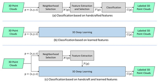
Figure 1.
Flowcharts of point cloud classification: (a) traditional methods based on handcrafted features; (b) deep learning method based on learned features; and (c) proposed method based on handcrafted and learned features.
Furthermore, in order to evaluate the applicability of the proposed method to different point cloud datasets, in this study, we conducted a classification and result analysis of the ALS and MLS point cloud data, respectively. Although both the scanning approaches generate point cloud data presented in the form of 3D coordinates, there is a vast distinction between their properties. While the ALS point cloud generally has a lower point density, higher acquisition speed, and a wider covering area, the MLS point cloud normally has a higher density and more distinct details. Another major distinction lies in the different scanning directions toward the ground objects. While the ALS scans are performed in a downward vertical direction at a high altitude, resulting in a sparse point cloud of the vertical plane of the ground objects (e.g., the walls of buildings), the MLS scans are conducted in a horizontal direction at the ground level toward the ground objects and may omit the points of the horizontal plane of several ground objects (e.g., the rooves of buildings).
3.1. Extraction of Handcrafted Features
The network architecture of PointNet indicates that it is characterised by its simple model, few parameters, and fast training speed, yet it is deficient in the extraction of local features. As a result, the handcrafted features used in this study were mainly the local features of the point cloud, for the purpose of making up for the deficiencies of PointNet. In addition, the intrinsic properties of the point cloud data, such as return intensity and elevation information, were utilised as features, whose effects on the classification efficacy were evaluated. Table 2 presents the handcrafted features used in this study. Their definition and calculation method are as follows.

Table 2.
List of various features used in the proposed method.
3.1.1. Covariance Features
Covariance features are the most representative type of common local features, and many researchers have confirmed their positive effect on classification [49,50,51]. The covariance features of point are generated mainly by calculating the (3 × 3) covariance matrix of the coordinates of all the points in its neighbourhood [51]. In this study, we first found the neighbourhood via K-nearest neighbours (KNN) and calculated the covariance matrix of all the points in the neighborhood. Then, by using eigen decomposition, we found the three eigenvalues of the covariance matrix, arranged from small to large as , and the three corresponding eigenvectors . Many geometric features can be derived from the eigenvalues, among which the three common shape features: linearity (L), planarity (P), and scattering (S), as proposed by Demantké, Mallet, David and Vallet [50], can be utilised to determine the shape behaviour of the points within the neighbourhood . Their calculation methods are illustrated in Formula (1) to Formula (3). When the point cloud in the neighbourhood was in a linear form, , while the value of linearity (L) was close to 1; when the point cloud in the neighbourhood was in a planar form, , and the value of planarity (P) was close to 1; when the point cloud in the neighbourhood was in a dispersed and volumetric form, , and the value of scattering (S) was close to 1. Furthermore, in this study, we used the verticality (V) put forth by Guinard and Landrieu [52]. The calculation method is illustrated in Formula (4). This verticality (V) was utilised to determine the verticality of the point distribution. The horizontal neighbourhood produced a value close to 0, while the vertical linear neighbourhood produced a value close to 1, and the vertical planar neighbourhood (e.g., façade) produced a median value ().
In addition, the normal vector of each point in the point cloud is generally regarded as one of the important features by many researchers [49]. The normal vector can be computed using many different calculation methods [53]. In this study, we used the eigen vector corresponding to the minimal eigenvalue in the covariance matrix of point as the normal vector N of the point and decomposed it along the 3D coordinate axes into three normal components serving as the normal features of the point, as demonstrated in Formula (5):
3.1.2. Height Features
Another effective feature involves elevation information of the point cloud. Both the ALS and the MLS data contain a large number of points on the ground surface. Almost all the other above-ground objects are connected to the ground, and the junction is where classification errors are most likely to occur. In order to solve this problem, many researchers filtered out the points on the ground before classifying the above-ground objects [54], while some introduced the height difference ∆z between the ground and the above-ground object as a feature for classification [38,40,54]. As the complete automation of the filtration of the points on the ground surface cannot be attained at the present stage, it remains a time-consuming and laborious task to thoroughly filter out the points on the ground [15]. In view of this, in this study, we utilised the height difference ∆z as the height feature, which was computed by subtracting the height of the lowest point in the scene from the height of the point.
3.1.3. Intensity Features
Apart from acquiring the 3D coordinates of the target point, the laser scanner occasionally records the return intensity I of the laser at the same time, the value of which may be affected by the texture and roughness of the target surface, the laser wavelength, the emitted energy, and the incidence angle, and therefore can facilitate classification to some extent [39,49].
3.2. Feature Selection and Model Configuration for ALS Point Cloud Classification
Figure 2a illustrates the ALS point cloud data utilised in this study. These test data constitute a subset of an ALS data collected over Tainan, Taiwan in August 2010. The data acquisition was carried out by the RIEGL-Q680i scanner, with a flight altitude of approximately 800 m and a point density of approximately 10 pt/m2. The primary application of this data was 3D urban mapping, and four different classes, including Ground, Building, Car, and Tree, were manually labelled beforehand and were utilised as the reference data for training and testing, as illustrated in Figure 2b. These test data contains a total of 2,262,820 points, and the number of points and percentage belonging to each class are shown in Table 3.
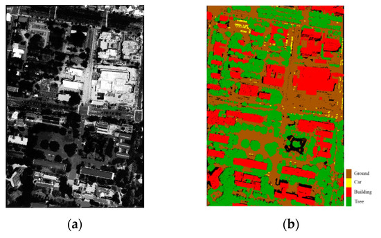
Figure 2.
Test area for the airborne laser scanning (ALS) point cloud dataset: (a) Point cloud data (displayed by intensity); (b) Labelled categories.

Table 3.
Number of points and percentage of each class for ALS point cloud.
On the basis of the two deep networks PointNet and PointNet++, in this study, we integrated a different type of handcrafted features discussed in the previous section into the ALS data and produced different models, as shown in Table 4.

Table 4.
PointNet and PointNet++ models with different features for ALS point cloud classification.
According to the design of the PointNet and PointNet++ models, the input point cloud was divided into several blocks first; then, a fixed number of points from each block were selected for training. Considering that the original study does not offer suggestions about the most ideal size of the blocks, in this study, we found the best block size via experiments (see Section 4.1 for details) and divided the ALS point cloud data into 15 m × 15 m blocks, with each block containing 2048 sampled points. The training strategy for the model basically corresponded with the setup suggested by the original study. The setting of the relevant hyperparameters is illustrated in Table 5. The definitions and effects of these hyperparameters can be found in [55].

Table 5.
Model configuration for PointNet and PointNet++.
Unlike the two aforementioned models that require the process of dividing the point cloud into blocks, KPConv directly conducts the classification of the point cloud of the scene. However, an excessive number of points might result in insufficient memory and subsequently lead to a failure in the calculation, hence the need for the subsampling of the original point cloud. Moreover, the convolution kernels in KPConv were classified as the rigid type and the deformable type. The training strategy for the model followed the setup from the original study, with a max epoch of 500, a batch size of 12, 15 kernel points, and the radius of influence of the point convolution set as 4 m [33].
3.3. Feature Selection and Model Configuration for MLS Point Cloud Classification
Figure 3a illustrates the MLS point cloud data utilised in this study. The test area is located at Tainan High Speed Rail Station District (Shulan) in Tainan, Taiwan. This MLS data were collected via the Optech Lynx-M1 scanner in December 2017, with a point density of approximately 200 pt/m2, and primarily used for road inventory and the production of HD maps. In comparison with the ALS data, the observed scene in the MLS data consisted of a larger number and greater complexity of ground objects and of the classifications of ground objects, including a total of eight classes: Ground, Tree, Street lamp, Traffic sign, Traffic light, Island (divisional island), Car, and Building, as shown in Figure 3b. There are 14,899,744 points in this observed scene, and the number of points and percentage belonging to each class is listed in Table 6.
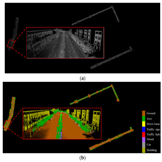
Figure 3.
Test area for the MLS point cloud dataset: (a) Point cloud data (displayed by intensity); (b) Labelled categories.

Table 6.
Number of points and percentage of each class for MLS point cloud.
On the basis of the two models PointNet and PointNet++, we tested different feature combinations for the MLS point cloud classification, as shown in Table 7, which differed from the ALS data with the additional intensity feature and removal of the normal features.

Table 7.
PointNet and PointNet++ models with different features for MLS point cloud classification.
In consideration of the dense point cloud and the large quantity of MLS data, in order to effectively acquire the local geometric features of the point cloud, we first executed subsampling and determined via experiments that the best block size was 5 m × 5 m, with 4096 points extracted from each block for training. The training strategy for the PointNet and PointNet++ models followed the setup from the original study. The setting of the relevant hyperparameters is illustrated in Table 8. The setup of KPConv basically resembled that described in Section 3.2. However, in view of the relatively complex scene and the relatively large number of point clouds in the MLS point cloud data, the max epoch was set to 600, while the batch size was set to 8.

Table 8.
Model parameters and corresponding values for PointNet and PointNet++.
3.4. Classification Performance Evaluation
In order to assess the efficacy of each model in point cloud classification, we used the classification performance metrics, which are frequently used in machine learning and include overall accuracy (OA), precision, recall, and F1-score, and Matthews correlation coefficient (MCC) [56]. The calculation of these indicators for binary classification can be expressed as follows:
Here, TP, FP, FN, and TN represent true positive, false positive, false negative, and true negative, respectively, all of which can be calculated from the point-based confusion matrix.
In the case of a multi-class problem with K classes, the macro-averaging procedure is commonly employed to calculate the overall mean of per-class measures for different indicators [57]. By this procedure, the precision, recall and F-1 score are computed for each class according to Equations (7)–(9), and then averaged via arithmetic mean. In addition, a multi-class extension of MCC in terms of the confusion matric was also considered in this study [58], which is defined as follows:
where c is the total number of samples correctly predicted, s is the total number of samples, is the number of samples that class k was predicted, and is the number of samples that class k truly occurred.
In comparison to the OA, the average F1-score is less vulnerable to the problem of imbalanced data. As a result, many studies have used the average F1-score in the assessment of the point cloud classification performance [14,18,59]. As an alternative measure unaffected by the imbalanced dataset issue, MCC_k is more informative than average F1-score and OA in evaluating classification problems [45,60]
4. Experimental Results
4.1. Effect of Block Size
When generally applied in image classification, CNN first partitions an image into many patches in order to extract the local features to be utilised in the classification. Similarly, the PointNet and PointNet++ models first partition the point cloud into numerous blocks, each of which serves as a unit during training. It is evident that the size of the blocks has a direct impact on the classification result. However, the original study on PointNet and PointNet++ does not offer specific suggestions about this concern. In order to conduct the succeeding experiments with the best block size, we partitioned the ALS data into blocks of five different sizes: , , , , and . We also conducted classification tests on the point cloud data before and after the addition of the geometric feature (L, P, S, V). The experimental results are shown in Figure 4, in which the triangles with dashed lines represent the classification results produced by using only the (x, y, z) coordinates, and the circles with solid lines represent the results produced after the addition of the geometric feature. Each color represents a different classification indicator, and the grey vertical bars indicate the calculation time required.
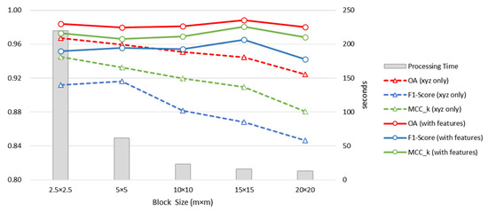
Figure 4.
Classification results of PointNet on ALS point clouds with different block sizes.
Figure 4 suggests that, prior to the addition of the geometric feature, the increase in the block size results in an evident decline in each classification indicator. This could be attributed to the fact that the larger blocks in the PointNet architecture resulted in the insufficiency of the local structures in the global features obtained via max pooling, hence the decrease in the classification efficacy [61]. However, note that when the blocks were in size, some of the indicators were lower than those following a block in size, which was likely to be associated with the size of the objects to be classified in the ALS point cloud. When a larger object was divided into numerous small pieces, its entire structure was destroyed, hence the inability of the network to learn the geometric structure of the object as a complete entity. In contrast, the classification results of the point cloud into which the geometric features were integrated (represented by the solid lines in Figure 4) indicated that the addition of the geometric features led to an increase in all of the classification indicators and that the block size had less impact on the classification, with the block size of generating a better classification result. As a result, in the succeeding experiments, the point cloud was partitioned into blocks of size . There was no overlap between blocks, and regions without point data were excluded. The construction following the completion of the partition is shown in Figure 5.
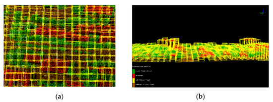
Figure 5.
Construction of non-overlapping blocks measuring for ALS point clouds: (a) Top view: (b) Side view.
Unlike the ALS point cloud data, the MLS data are characterised by a high point density and a small object scale. Theoretically, the blocks should be smaller in size if the local geometric structures of the point cloud in each block are to be effectively extracted. In view of this, we conducted experiments using blocks of four sizes:, , , and . Figure 6 illustrates the classification results of the point cloud data before and after the addition of the features. According to the classification results produced after the addition of the geometric features, the classification performance following the blocks measuring was similar to that following the blocks measuring . However, the smaller the size of the blocks was, the longer was the calculation time required. As a result, we conducted the succeeding experiment by using the blocks measuring . The construction following the completion of partition is shown in Figure 7.
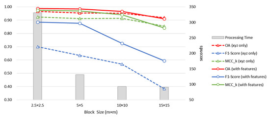
Figure 6.
Classification results of PointNet on MLS point clouds with different block sizes.

Figure 7.
Construction of non-overlapping blocks measuring for MLS point clouds: (a) Top view: (b) Side view.
4.2. Classification Results for ALS Point Clouds
4.2.1. Effects of the Handcrafted Features Using PointNet
In this section, we focused on assessing the influence of the addition of the handcrafted features to the ALS point cloud data on the classification efficacy of PointNet. As shown in Table 4, following the addition of different types of features to the original point cloud coordinates, 80% of the data were utilised in training, while 20% were utilised in testing. The hyperparameters for model training are illustrated in Table 5, and the classification results are illustrated in Figure 8, in which the classification indicators, including overall accuracy, average recall, average precision, average F1-score, and MCC_k, are displayed in column charts for the purpose of easy comparison. Overall, the classification results generated after the addition of the features surpassed those produced using only the (x, y, z) coordinates. While the ALS_PointNet_2 model with the addition of normal features effectively improves the average recall, it resulted in a decrease in the average precision. In contrast, ALS_PointNet_3, to which three eigenvalues were added, and ALS_PointNet_4, to which the shape features (L, P, S) were added, have a noticeable increase in both the average recall and the average precision. However, with the inclusion of the verticality (V) feature (i.e., ALS_PointNet_5), the average recall increased, while the average precision decreased. Furthermore, while the classification results of ALS_PointNet_6, to which the normal vector (Nx, Ny, Nz) and the covariance feature (L, P, S, V) were simultaneously added, did not exhibit distinct differences from those of ALS_PointNet_4. Finally, the study produced ALS_PointNet_7 by adding the height feature to ALS_PointNet_4, which resulted in a slight enhancement in the classification results.

Figure 8.
Comparison of classification results using PointNet with different handcrafted features on ALS point clouds.
4.2.2. Effects of the Handcrafted Features Using PointNet++
The experiment focused on assessing the influence of the addition of the handcrafted features to PointNet++ on the classification efficacy of the ALS point cloud, by adding features identical to those used in the previous experiment (as shown in Table 4). Table 5 shows the training hyperparameters of the model, with 80% of the data utilised in training and 20% utilised in testing. The testing result is illustrated in Figure 9. Similar to the PointNet model, specifically adding normal features (ALS_PointNet++_2) does not improve the classification efficacy noticeably. In contrast, the addition of the eigenvalues (ALS_PointNet++_3) or the shape features (ALS_PointNet++_4) could enhance the overall classification results, but only to a limited extent. Even if different types of handcrafted features are included in the PointNet++ (ALS_PointNet++_5 and ALS_PointNet++_6), some classification indicators decreased rather than increased. It is worth noting that when height features are added to the model (ALS_PointNet++_7), all classification metrics were improved and the best classification results were achieved compared to other models.

Figure 9.
Comparison of classification results using PointNet++ with different handcrafted features on ALS point clouds.
4.2.3. Comparison with other Methods
This section compares the classification results generated via the method proposed in this paper, RF, and KPConv. RF is the classification approach in machine learning provided by the commercial software LiDAR360, with its input including the point cloud coordinates (x, y, z) and the covariance features (L, P, S, V). PointNet utilised ALS_PointNet_5, to which the covariance features (L, P, S, V) were added, and was represented by PointNet(F). With respect to PointNet++, because of the limited effects of the additional features, ALS_PointNet++_1, to which no feature was added, was utilised and represented by the same name PointNet++. Lastly, the deformable KPConv was executed with the influence distance of 4 m. In order to maintain an identical testing environment for the four methods, the experiment reselected the training and testing samples. The classification results are illustrated in Figure 10. In terms of OA, PointNet(F), to which the handcrafted features were added, produced the best result, while RF came in second but exhibited the lowest average precision. In terms of the F1-score, PointNet(F) produced the best result, and KPConv came in second. In terms of MCC_k, PointNet(F) still performed the best, followed by RF. The experimental results indicated that when equipped with the handcrafted features, PointNet was indeed effective in enhancing the classification efficacy of the ALS data, which possessed a lower point density and a smaller number of classes, and could even surpass other more complex models, such as PointNet++ and KPConv.
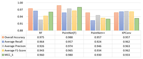
Figure 10.
Comparison of classification results on ALS point clouds using RF and three deep learning models.
4.3. Classification Results for MLS Point Cloud
4.3.1. Effects of Handcrafted Features Using PointNet
The main focus of the experiment was to assess the influence of the addition of the handcrafted features to PointNet on the classification result of the MLS point cloud, by using a strategy similar to that applied to the classification of the ALS point cloud data. The MLS_PointNet_1 to MLS_PointNet_5 models were devised by adding different types of features to the MLS point cloud data (as shown in Table 7). Training and testing for each model were then conducted. The classification results are illustrated in Figure 11. According to the results, after the addition of the features, there was a noticeable increase in each of the indicators of the classification result. MLS_PointNet_4, to which intensity feature I and the covariance features (L, P, S, V) were added, produced the best result. In comparison to the result produced without the addition of any feature (MSL_PointNet_1), the average recall of MLS_PointNet_4 increased by 0.271, average precision by 0.203, overall accuracy by 0.032, and the F1-score by 0.260, altogether showing substantial advancement. In contrast, MLS_PointNet_5, which was formed with the addition of the height features to MLS_PointNet_4, resulted in a decrease in the average precision and was of no benefit to the classification result.
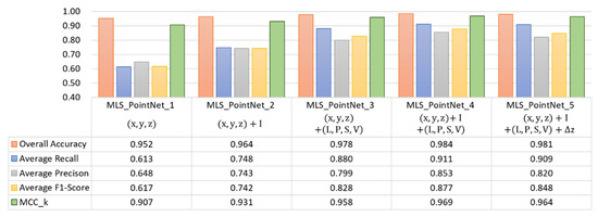
Figure 11.
Comparison of classification results using PointNet with different handcrafted features on MLS point clouds.
4.3.2. Effects of Handcrafted Features Using PointNet++
This section mainly focuses on testing the influence of the addition of different features to PointNet++ on the classification efficacy of the MLS point cloud, by adding the features identical to those in the PointNet experiment discussed in the previous section. The classification results are illustrated in Figure 12. In comparison to the MLS_PointNet++_1 model, in which only the point coordinates were used as the input, the addition of either intensity feature I or the covariance features (L, P, S, V) could increase each of the classification indicators only to a limited extent, with some of them even declining. The experimental results indicated that the self-learned local features of PointNet++ have already been effective in processing a complex scene with a higher point density and a larger number of classes; thus, the inclusion of the handcrafted features could produce very limited benefits. In addition, it can be found that height features are not beneficial for MLS point cloud classification.
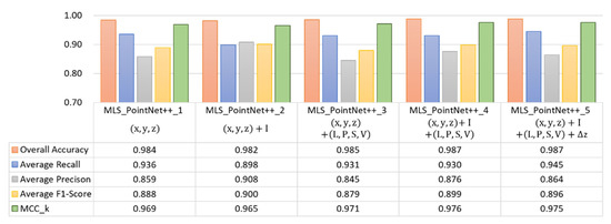
Figure 12.
Comparison of classification results using PointNet++ with different handcrafted features on MLS point clouds.
4.3.3. Comparison with other Methods
This section compares the experimental result of the proposed method with the classification results of RF and KPConv. The input of RF consisted of the original point coordinates (x, y, z), the covariance features (L, P, S, V), and the intensity (I). PointNet used MLS_PointNet_4 equipped with the additional covariance features (L, P, S, V) and the intensity (I), and is here represented by PointNet(F). PointNet++ used MLS_PointNet++_1, to which no feature was added. For deformable KPConv, the kernel points influence distance was set as equal to 4 m. The classification results are shown in Figure 13. In terms of OA, each method generated a satisfactory result. In terms of the F1-score, RF produced the worst result, while PointNet(F) and PointNet++ produced very similar classification results, and KPConv produced the best result. In terms of MCC_k, KPConv performed the best, followed by PointNet and PointNet++, and RF had the worst results.
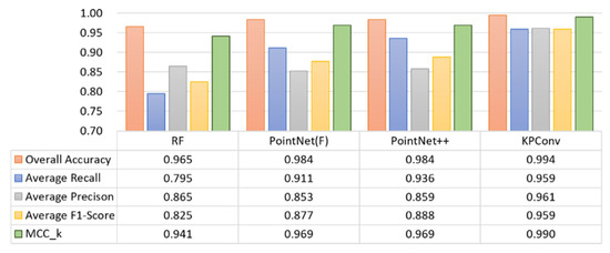
Figure 13.
Comparison of classification results on MLS point clouds using RF and three deep learning models.
5. Discussion
5.1. Effects of Handcraft Features for PointNet
For the PointNet model, the experimental results illustrated in Figure 8 and Figure 11 showed that the classification performance for ALS and MLS point cloud data can be improved regardless of which type of handcrafted features introduced in Section 3.1 were added. Moreover, the amount of improvement in classification performance apparently depends on the selected handcrafted features. In this section, we will discuss the classification results of PointNet with respect to the properties of the selected handcrafted features.
The normalized confusion matrix of the classification result for ALS point cloud shown in Table 9 indicates that the main problem of the PointNet without handcrafted features is the low recall value of the class of Car. In addition, there is ambiguity between the classes of Building and Tree. While the normal features are included in ALS_PointNet_2, the problem of cars being misclassified as ground and buildings has been improved. The presumed reason should be that the normal represents the direction of a surface, and all surface normals of a car vary more than the normals of the ground or a building. However, this could lead to trees with rough surfaces being misclassified as cars, resulting in low precision of the class of Car. In contrast, ALS_PointNet_3, to which three eigenvalues were added, provided the local distribution information of the point cloud and therefore led to a noticeable increase in both the average F-1 score and the . The shape features (L, P, S) in ALS_PointNet_4 were essentially the conversion results of the three eigenvalues, and therefore have similar classification results as ALS_PointNet_3. Once the verticality (V) feature was added (i.e., ALS_PointNet_5), the average recall increased, while the average precision decreased. Furthermore, while the classification results of ALS_PointNet_6, to which the normal vector (Nx, Ny, Nz) and the covariance feature (L, P, S, V) were simultaneously added, did not exhibit distinct differences from those of ALS_PointNet_4, the addition of more features resulting in a longer training time. Finally, the study produced ALS_PointNet_7 by adding the height feature to ALS_PointNet_4, which resulted in a slight enhancement in the classification results. In most cases, the height features were generally added for reducing the interference from the points on the ground. Nevertheless, most of the classification errors caused by the points on the ground had already been rectified in the ALS_PointNet_4 model, to which (L, P, S) was added, hence the limited beneficial result generated by the addition of the height features.

Table 9.
Normalized Confusion matrix of ALS_PointNet_1 (%).
In order to demonstrate the practical benefits produced by the handcrafted features for PointNet model, here, we compared ALS_PointNet_1, to which no feature was added, and ALS_PointNet_4, to which the shape features (L, P, S) were added. Table 9 and Table 10 illustrate the normalized confusion matrix of the classification result of each model, respectively. Note that the addition of the shape features (L, P, S) considerably rectified the problem of misclassification, i.e., the buildings being misclassified as the trees or the grounds, the grounds being misclassified as the buildings and the trees, and the trees being misclassified as the buildings. Moreover, the recall of the class of Car considerably increased by approximately 8.5% after the addition of the features. The visualized classification results of the two models are shown in Figure 14 and Figure 15. In Figure 14, note that the overall classification errors considerably decreased after the addition of the features, with only a few classification errors still occurring on the periphery of a small number of buildings. Figure 15a indicates that after the addition of the features, the problem of the buildings being misclassified as trees was rectified. Figure 15b indicates that prior to the addition of the feature, misclassification was likely to occur at the junction of the edge of the buildings and the trees. Nevertheless, such problems were rectified after the addition of the features.

Table 10.
Normalized Confusion matrix of ALS_PointNet_4 (%).
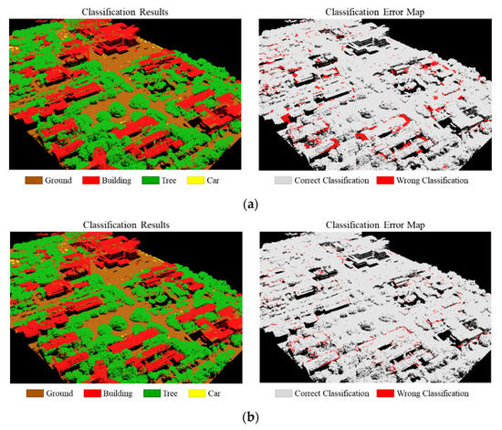
Figure 14.
Comparison of classification results on ALS point clouds: (a) Classification results and error map of ALS_PointNet_1; (b) Classification results and error map of ALS_PointNet_4.
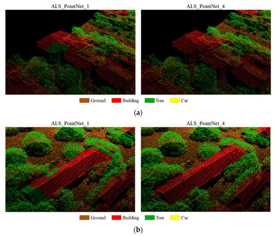
Figure 15.
Classification efficacy of PointNet after the addition of features (left: ALS_PointNet_1; right: ALS_PointNet_4): (a) Lower degree of misclassification of the buildings as the trees; (b) Lower degree of misclassification at the junction of the edge of the buildings and the trees.
When PointNet model with handcrafted features was applied to the MLS point cloud, there was also a significant improvement in all metrics of the classification results, as shown in Figure 11. Both intensity features and shape features are beneficial for MLS point cloud classification, with shape features being the more effective. When they are added to the model together, i.e., MLS_PointNet_4, better classification results were obtained than when they were added separately. This is due to the fact that intensity and shape features are essentially independent of each other. In contrast, adding the height feature to the PointNet model is unproductive for point cloud classification. This is similar to the case of ALS point cloud classification.
To further discuss the classification results for each class, Table 11 and Table 12 present the normalized confusion matrices for MLS_PointNet_1 and MLS_PointNet_4 respectively. The results in Table 11 showed that MLS_PointNet_1, to which no handcrafted features were added, had some problems with misclassification, including the pole-like objects such as street lamps, traffic signs, and traffic lights being misclassified as trees; some cars being classified as trees, islands, and ground; and many buildings being misclassified as trees. The recall and precision values for Traffic sign were only 0.127 and 0.054, respectively, which were the worst classification results in the entire MLS scene. However, with the addition of intensity and shape features, all the overall classification metrics increased, and most of the above problems of misclassification were significantly improved. For example, the recall value of Traffic sign improved from 0.127 to 0.915, and the precision value improved from 0.054 to 0.656. In addition, the recall values of Street light, Car and Building improved from 0.321, 0.509 and 0.577 to 0.865, 0.913 and 0.900 respectively. Although the addition of the features has significantly improved the classification efficacy for MLS point cloud, there are still some problems, such as some traffic lights being misclassified as traffic signs and trees being misidentified as traffic lights, resulting in low precision values of Traffic sign and Traffic light.

Table 11.
Normalized Confusion matrix of MLS_PointNet_1.

Table 12.
Normalized Confusion matrix of MLS_PointNet_4.
5.2. Effects of Handcraft Features for PointNet++
Because the PointNet++ model essentially has the ability to extract local features, the addition of the shape features yields limited benefits in both ALS and MLS point cloud classification, as illustrated in Figure 9 and Figure 12 respectively. It is worth noting that height features are beneficial for ALS data classification, but not for MLS data. This was presumably due to the fact that the ALS point cloud had fewer points in the vertical surface, making the height information somewhat distinguishable between classes. Although the average F-1 score and MCC did not improve much after adding handcrafted features for the MLS point cloud, the classification accuracy of some pole-like objects, such as traffic signs and traffic lights, was improved significantly. An example is shown in Figure 16a, where a portion of Traffic light is misclassified as ground, which was improved by adding height features, as shown in Figure 16b. This demonstrated that the learning features of PointNet++ are still inadequate for the interpretation of pole-like objects, but the handcrafted features included in this study can moderately compensate for this weakness. However, it was also found that the inclusion of handcrafted features reduced the precision values of some individual classes, which is an issue that could be improved by future research.
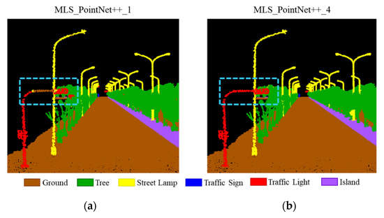
Figure 16.
Comparison of classification results on MLS point clouds: (a) MLS_PointNet++_1; (b) MLS_PointNet++_5. The height feature is helpful to rectify the misclassification of the long, thin pole of the traffic light as the ground.
5.3. Comparison with other Methods
The classification results of Figure 10 in Section 4.2.3 were compared via visualization, as shown in Figure 17. RF erred in misclassifying the buildings as the trees or the cars, while the errors made by PointNet(F) mostly occurred at the junction of a building and a tree. Despite the addition of specific geometric features, some of the more detailed local structures of the point cloud could still not be captured. In comparison to PointNet++ and KPConv, PointNet(F) was less likely to result in classification errors related to large area on ground surface or buildings’ rooves. While PointNet++ could rectify the problem of the periphery of the building being misclassified as the tree in PointNet via the self-learned local features, it resulted in the points on the ground on a large scale being misclassified as the buildings, and buildings with an irregular structure being misclassified as the trees. Lastly, while KPConv could acquire more detailed features via point convolution and was less likely to produce classification errors on the periphery of objects, as confirmed by the experiment, it often misclassified a large roof of a building as the ground, which was a problem that might be associated with the location of the kernel points and the kernel size of convolution.
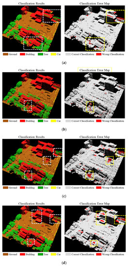
Figure 17.
Classification results of RF and DL models on ALS point cloud with four classes: (a) Classification results of RF; (b) Classification results of PointNet(F); (c) Classification results of PointNet++; (d) Classification results of KPConv.
Figure 18 shows a comparison of the visualized classification results on MLS point clouds using RF and three deep learning models. In terms of the classes of Ground, Tree, and Car, each model produced a satisfactory result. However, in terms of the identification of other classes, the models displayed varying degrees of false positive rates. By comparing the reference data in Figure 18a,b, a large number of divisional islands were misclassified as the ground points by RF, while buildings were misclassified as trees. In Figure 18c,d, although many incorrect classifications by RF were noticeably rectified in PointNet and PointNet++, some problems remained unsolved, such as the street lamps and the traffic lights being misclassified as the trees, as well as the inaccuracy in classifying the traffic signs of a smaller size and with a smaller number of points. In comparison to PointNet, PointNet++ took the more detailed local features into account and was therefore less likely to misclassify the traffic lights as the street lamps, yet it still made misclassifications in detecting pole-like objects. Finally, with respect to KPConv, as shown in Figure 18e, while it produced the best classification result in the identification of each class, such as the divisional islands and the traffic signs, a few faults could still be found in its identification of the walls of the buildings.
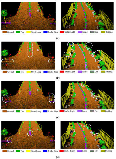
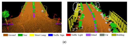
Figure 18.
Classification results of RF and DL models on MLS point cloud with eight classes: (a) Labelled categories (ground truth); (b) Classification results of RF; (c) Classification results of PointNet(F); (d) Classification results of PointNet++; (e) Classification results of KPConv.
5.4. Comparison of Computational Efficiency
Finally, we compared the calculation time and the classification efficacy of the deep learning models used in this study. Table 13 shows the calculation time that each model required per 100 epochs. In this table, PointNet(F) represents the proposed PointNet model with handcrafted features, and PointNet, PointNet++ and KPConv are the deep learning models with no features added. Figure 19 illustrates and compares the classification results and the training time of each model for the ALS and the MLS point cloud data. As indicated by the figures, the calculation time required for PointNet(F) did not increase much after adding the handcrafted features, but its classification performance has significantly been improved. Furthermore, PointNet(F) produced the best classification result and required little calculation time for the simple ALS scene, while KPConv produced the best classification result but required a large amount of calculation time for the complex MLS scene. In contrast, the classification efficiency and efficacy of PointNet++ for the MLS scene was relatively balanced. As a result, in terms of classification for a simple scene or a situation equipped with adequate prior knowledge for feature extraction, PointNet(F) would be more beneficial in practical applications.

Table 13.
Training time per 100 epochs of different models (seconds).
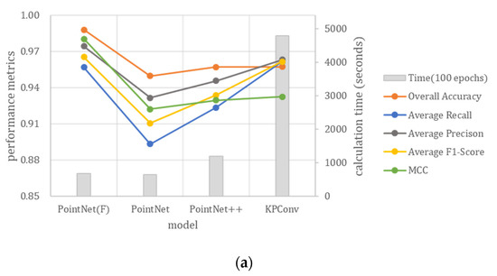
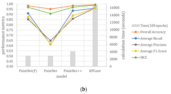
Figure 19.
Comparison of classification results and computational efficiency of the deep learning models: (a) ALS point cloud; (b) MLS point cloud.
6. Summary and Conclusions
This study focused on the two deep learning networks PointNet and PointNet++, and analyzed the effects of the addition of various type of handcrafted features on the point cloud classification efficacy. In addition, two point cloud datasets, including an ALS dataset covering a simple scene and an MLS dataset covering a complex scene, are used to test the performance of the proposed method.
In terms of the PointNet model, the various types of handcrafted features introduced in this study are clearly useful for classifying ALS and MLS point cloud data. In particular, the shape features that contain local geometric structure information have the most significant improvement in the classification performance of point clouds. For ALS point cloud classification, the addition of the shape features considerably rectified the problem of misclassification, i.e., the buildings being misclassified as the trees or the grounds, the grounds being misclassified as the buildings and the trees, and the trees being misclassified as the buildings. For MLS point clouds, the problem of misclassification of pole-like objects such as street lamps, traffic signs, and traffic lights can be significantly rectified by adding intensity and shape features to the PointNet model. In addition, the inclusion of these local features also effectively solves the problem of cars and buildings being misclassified as trees. In terms of PointNet++, despite its intrinsic ability to extract local features, the addition of the handcrafted features could facilitate the classification performance to a little extent for both ALS and MLS data. In addition, we find that height features are beneficial for ALS data classification, but not for MLS data. This should be due to the different point distributions between ALS and MLS point clouds.
By comparing the aforementioned results with the results produced by RF and KPConv, we found that PointNet, with the addition of the features, performed better in the case of the ALS data, while KPConv, equipped with the 3D convolution kernel, performed better in the case of the complex MLS data, but had a complex model architecture and required a considerable amount of calculation time. With the addition of local features, PointNet could attain results in the MLS data classification similar to those produced by PointNet++ and KPConv, but with the advantages of a simple model architecture and a short calculation time. As a result, the PointNet model incorporating handcrafted features will be more beneficial for practical applications in classifying simple observed scenes or analyzing complex scenes efficiently.
Through the experiments, we found that there is ample room for discussion and improvement. First, in terms of the influence of the number of ground object classifications, take the ALS data used in this study for example; while only four types of ground objects were classified in the experiment, many scenes in reality might be considerably more complex. Therefore, testing and discussions on more complex ALS scenes containing more ground object classifications should be conducted in the future. Furthermore, through practical applications, we observed that in the cases of both the ALS and the MLS data, the ground points occupied a majority of the data and, consequently, resulted in the problem of data imbalance. If this problem is solved, better results and performance can be expected. Finally, in this study, we tested only some point-based features. Discussions on the efficacy of other features, such as contextual-based features [54], object-based features [22], and full-waveform features [38], should be carried out in the future.
Author Contributions
P.-H.H. originally proposed the idea of incorporating handcrafted features into deep learning for point cloud classification; he also guided the study and experiment design, and contributed to manuscript writing and revision. Z.-Y.Z. contributed to the codes of the algorithm, experiments implementation, and partial paper writing. All authors have read and agreed to the published version of the manuscript.
Funding
This research was funded by the Ministry of Science and Technology, Taiwan, grant number 108-2621-M-002-005-.
Acknowledgments
The authors thanks Chung Hsing Surveying Co., Ltd. and Strong Engineering Consulting Co., Ltd. for providing the point cloud data used in this study.
Conflicts of Interest
The authors declare no conflict of interest.
References
- Aguilar, F.J.; Mills, J.P. Accuracy assessment of lidar-derived digital elevation models. Photogramm. Rec. 2008, 23, 148–169. [Google Scholar] [CrossRef]
- Sohn, G.; Dowman, I.J. A model-based approach for reconstructing a terrain surface from airborne LIDAR data. Photogramm. Rec. 2008, 23, 170–193. [Google Scholar] [CrossRef]
- Vosselman, G.; Kessels, P.; Gorte, B. The utilisation of airborne laser scanning for mapping. Int. J. Appl. Earth Obs. Geoinformation 2005, 6, 177–186. [Google Scholar] [CrossRef]
- Schwarz, B. Mapping the world in 3D. Nat. Photon 2010, 4, 429–430. [Google Scholar] [CrossRef]
- Guo, Y.; Bennamoun, M.; Sohel, F.; Lu, M.; Wan, J. An Integrated Framework for 3-D Modeling, Object Detection, and Pose Estimation from Point-Clouds. IEEE Trans. Instrum. Meas. 2015, 64, 683–693. [Google Scholar] [CrossRef]
- Mahler, J.; Matl, M.; Satish, V.; Danielczuk, M.; Derose, B.; McKinley, S.; Goldberg, K. Learning ambidextrous robot grasping policies. Sci. Robot. 2019, 4, eaau4984. [Google Scholar] [CrossRef]
- Lim, K.; Treitz, P.; Wulder, M.; St-Onge, B.; Flood, M. LiDAR remote sensing of forest structure. Prog. Phys. Geogr. Earth Environ. 2003, 27, 88–106. [Google Scholar] [CrossRef]
- Zhang, Z.; Liu, X. Support vector machines for tree species identification using LiDAR-derived structure and intensity variables. Geocarto Int. 2013, 28, 364–378. [Google Scholar] [CrossRef]
- Gomes, L.; Bellon, O.R.P.; Silva, L. 3D reconstruction methods for digital preservation of cultural heritage: A survey. Pattern Recognit. Lett. 2014, 50, 3–14. [Google Scholar] [CrossRef]
- Rodríguez-Gonzálvez, P.; Fernández-Palacios, B.J.; Muñoz-Nieto, A.; Arias, P.; González-Aguilera, D. Mobile LiDAR System: New Possibilities for the Documentation and Dissemination of Large Cultural Heritage Sites. Remote Sens. 2017, 9, 189. [Google Scholar] [CrossRef]
- Guan, H.; Li, J.; Cao, S.; Yu, Y. Use of mobile LiDAR in road information inventory: A review. Int. J. Image Data Fusion 2016, 7, 219–242. [Google Scholar] [CrossRef]
- Balado, J.; Martínez-Sánchez, J.; Arias, P.; Novo, A. Road Environment Semantic Segmentation with Deep Learning from MLS Point Cloud Data. Sensors 2019, 19, 3466. [Google Scholar] [CrossRef] [PubMed]
- Seif, H.G.; Hu, X. Autonomous Driving in the iCity—HD Maps as a Key Challenge of the Automotive Industry. Engineering 2016, 2, 159–162. [Google Scholar] [CrossRef]
- Zhao, R.; Pang, M.; Wang, J. Classifying airborne LiDAR point clouds via deep features learned by a multi-scale convolutional neural network. Int. J. Geogr. Inf. Sci. 2018, 32, 960–979. [Google Scholar] [CrossRef]
- Li, W.; Wang, F.-D.; Xia, G.-S. A geometry-attentional network for ALS point cloud classification. ISPRS J. Photogramm. Remote Sens. 2020, 164, 26–40. [Google Scholar] [CrossRef]
- Weinmann, M.; Jutzi, B.; Hinz, S.; Mallet, C. Semantic point cloud interpretation based on optimal neighborhoods, relevant features and efficient classifiers. ISPRS J. Photogramm. Remote Sens. 2015, 105, 286–304. [Google Scholar] [CrossRef]
- Grilli, E.; Menna, F.; Remondino, F. A REVIEW OF POINT CLOUDS SEGMENTATION AND CLASSIFICATION ALGORITHMS. ISPRS Int. Arch. Photogramm. Remote Sens. Spat. Inf. Sci. 2017, 339–344. [Google Scholar] [CrossRef]
- Yang, Z.; Jiang, W.; Xu, B.; Zhu, Q.; Jiang, S.; Huang, W. A Convolutional Neural Network-Based 3D Semantic Labeling Method for ALS Point Clouds. Remote Sens. 2017, 9, 936. [Google Scholar] [CrossRef]
- Aijazi, A.K.; Checchin, P.; Trassoudaine, L. Segmentation Based Classification of 3D Urban Point Clouds: A Super-Voxel Based Approach with Evaluation. Remote Sens. 2013, 5, 1624–1650. [Google Scholar] [CrossRef]
- Mongus, D.; Lukač, N.; Žalik, B. Ground and building extraction from LiDAR data based on differential morphological profiles and locally fitted surfaces. ISPRS J. Photogramm. Remote Sens. 2014, 93, 145–156. [Google Scholar] [CrossRef]
- El-Ashmawy, N.; Shaker, A. Raster vs. Point Cloud LiDAR Data Classification. ISPRS Int. Arch. Photogramm. Remote Sens. Spat. Inf. Sci. 2014, XL-7, 79–83. [Google Scholar] [CrossRef]
- Kim, H.B.; Sohn, G. Random Forests Based Multiple Classifier System for Power-Line Scene Classification. ISPRS Int. Arch. Photogramm. Remote Sens. Spat. Inf. Sci. 2011, XXXVIII-5/W12, 253–258. [Google Scholar] [CrossRef]
- Weinmann, M.; Schmidt, A.; Mallet, C.; Hinz, S.; Rottensteiner, F.; Jutzi, B. Contextual Classification of Point Cloud Data by Exploiting Individual 3d Neigbourhoods. ISPRS Ann. Photogramm. Remote Sens. Spat. Inf. Sci. 2015, II-3/W4, 271–278. [Google Scholar] [CrossRef]
- Guo, B.; Huang, X.; Zhang, F.; Sohn, G. Classification of airborne laser scanning data using JointBoost. ISPRS J. Photogramm. Remote Sens. 2015, 100, 71–83. [Google Scholar] [CrossRef]
- Lecun, Y.; Bengio, Y.; Hinton, G. Deep learning. Nature 2015, 521, 436–444. [Google Scholar] [CrossRef]
- Liu, W.; Sun, J.; Li, W.; Hu, T.; Wang, P. Deep Learning on Point Clouds and Its Application: A Survey. Sensors 2019, 19, 4188. [Google Scholar] [CrossRef]
- Charles, R.Q.; Su, H.; Kaichun, M.; Guibas, L.J. PointNet: Deep Learning on Point Sets for 3D Classification and Segmentation. In Proceedings of the 2017 IEEE Conference on Computer Vision and Pattern Recognition (CVPR), Honolulu, HI, USA, 21–26 July 2017; pp. 77–85. [Google Scholar]
- Hu, X.; Yuan, Y. Deep-Learning-Based Classification for DTM Extraction from ALS Point Cloud. Remote Sens. 2016, 8, 730. [Google Scholar] [CrossRef]
- Maturana, D.; Scherer, S. VoxNet: A 3D Convolutional Neural Network for real-time object recognition. In Proceedings of the 2015 IEEE/RSJ International Conference on Intelligent Robots and Systems (IROS), Hamburg, Germany, 28 September–2 October 2015; pp. 922–928. [Google Scholar]
- Qi, C.R.; Yi, L.; Su, H.; Guibas, L.J. PointNet++: Deep Hierarchical Feature Learning on Point Sets in a Metric Space. In Proceedings of the 31st International Conference on Neural Information Processing Systems (NIPS 2017), Long Beach, CA, USA, 4–9 December 2017; pp. 5105–5114. [Google Scholar]
- Li, Y.; Bu, R.; Sun, M.; Wu, W.; Di, X.; Chen, B. PointCNN: Convolution on X-Transformed Points. In Proceedings of the 32nd Conference on Neural Information Processing Systems (NeurIPS 2018), Montréal, QC, Canada, 3–8 December 2018. [Google Scholar]
- Jiang, M.; Wu, Y.; Lu, C. PointSIFT: A SIFT-like Network Module for 3D Point Cloud Semantic Segmentation. arXiv 2018, arXiv:1807.00652. [Google Scholar]
- Thomas, H.; Qi, C.R.; Deschaud, J.-E.; Marcotegui, B.; Goulette, F.; Guibas, L. KPConv: Flexible and Deformable Convolution for Point Clouds. In Proceedings of the 2019 IEEE/CVF International Conference on Computer Vision (ICCV), Seoul, Korea, 27 October–2 November 2019; pp. 6410–6419. [Google Scholar]
- Arief, H.A.; Indahl, U.G.; Strand, G.-H.; Tveite, H. Addressing overfitting on point cloud classification using Atrous XCRF. ISPRS J. Photogramm. Remote Sens. 2019, 155, 90–101. [Google Scholar] [CrossRef]
- Zhang, J.; Zhao, X.; Chen, Z.; Lu, Z. A Review of Deep Learning-Based Semantic Segmentation for Point Cloud. IEEE Access 2019, 7, 179118–179133. [Google Scholar] [CrossRef]
- Bello, S.A.; Yu, S.; Wang, C.; Adam, J.M.; Li, J. Review: Deep Learning on 3D Point Clouds. Remote Sens. 2020, 12, 1729. [Google Scholar] [CrossRef]
- Liu, H. Feature Engineering for Machine Learning and Data Analytics; CRC Press: Boca Raton, FL, USA, 2018; p. 418. [Google Scholar]
- Mallet, C.; Bretar, F.; Roux, M.; Soergel, U.; Heipke, C. Relevance assessment of full-waveform lidar data for urban area classification. ISPRS J. Photogramm. Remote Sens. 2011, 66, S71–S84. [Google Scholar] [CrossRef]
- Zhang, J.X.; Lin, X.; Ning, X. SVM-Based Classification of Segmented Airborne LiDAR Point Clouds in Urban Areas. Remote Sens. 2013, 5, 3749–3775. [Google Scholar] [CrossRef]
- Chehata, N.; Guo, L.; Mallet, C. Airborne LiDAR Feature Selection for Urban Classification Using Random Forests. Int. Arch. Photogramm. Remote Sens. Spat. Inf. Sci. 2009, XXXVIII-3/W8, 207–212. [Google Scholar]
- Yan, L.; Li, Z.; Liu, H.; Tan, J.; Zhao, S.; Chen, C. Detection and classification of pole-like road objects from mobile LiDAR data in motorway environment. Opt. Laser Technol. 2017, 97, 272–283. [Google Scholar] [CrossRef]
- Lodha, S.K.; Fitzpatrick, D.M.; Helmbold, D.P. Aerial Lidar Data Classification using AdaBoost. In Proceedings of the Sixth International Conference on 3-D Digital Imaging and Modeling (3DIM 2007); Institute of Electrical and Electronics Engineers (IEEE), Montreal, QC, Canada, 21–23 August 2007; pp. 435–442. [Google Scholar]
- Bhattacharya, D.; Pillai, S.; Antoniou, A. Waveform classification and information extraction from LIDAR data by neural networks. IEEE Trans. Geosci. Remote Sens. 1997, 35, 699–707. [Google Scholar] [CrossRef]
- Höfle, B.; Hollaus, M.; Hagenauer, J. Urban vegetation detection using radiometrically calibrated small-footprint full-waveform airborne LiDAR data. ISPRS J. Photogramm. Remote Sens. 2012, 67, 134–147. [Google Scholar] [CrossRef]
- Plaza-Leiva, V.; Gómez-Ruiz, J.; Mandow, A.; García-Cerezo, A. Voxel-Based Neighborhood for Spatial Shape Pattern Classification of Lidar Point Clouds with Supervised Learning. Sensors 2017, 17, 594. [Google Scholar] [CrossRef]
- Schmohl, S.; Sörgel, U. Submanifold sparse convolutional networks for semantic segmentation of large-scale als point clouds. ISPRS Ann. Photogramm. Remote Sens. Spat. Inf. Sci. 2019, 77–84. [Google Scholar] [CrossRef]
- Qi, C.R.; Su, H.; NieBner, M.; Dai, A.; Yan, M.; Guibas, L.J. Volumetric and Multi-view CNNs for Object Classification on 3D Data. In Proceedings of the 2016 IEEE Conference on Computer Vision and Pattern Recognition (CVPR), Las Vegas, NV, USA, 27–30 June 2016; pp. 5648–5656. [Google Scholar]
- Su, H.; Maji, S.; Kalogerakis, E.; Learned-Miller, E. Multi-view Convolutional Neural Networks for 3D Shape Recognition. In Proceedings of the 2015 IEEE International Conference on Computer Vision (ICCV), Santiago, Chile, 7–13 December 2015; pp. 945–953. [Google Scholar]
- Yang, B.; Dong, Z. A shape-based segmentation method for mobile laser scanning point clouds. ISPRS J. Photogramm. Remote Sens. 2013, 81, 19–30. [Google Scholar] [CrossRef]
- Demantké, J.; Mallet, C.; David, N.; Vallet, B. DIMENSIONALITY BASED SCALE SELECTION IN 3D LIDAR POINT CLOUDS. ISPRSInt. Arch. Photogramm. Remote Sens. Spat. Inf. Sci. 2012, XXXVIII-5/W12, 97–102. [Google Scholar] [CrossRef]
- LaLonde, J.-F.; Vandapel, N.; Huber, D.F.; Hebert, M. Natural terrain classification using three-dimensional ladar data for ground robot mobility. J. Field Robot. 2006, 23, 839–861. [Google Scholar] [CrossRef]
- Guinard, S.; Landrieu, L. Weakly supervised segmentation-aided classification of urban scenes from 3d lidar point clouds. ISPRS Int. Arch. Photogramm. Remote Sens. Spat. Inf. Sci. 2017, XLII-1/W1, 151–157. [Google Scholar] [CrossRef]
- Zhao, R.; Pang, M.; Liu, C.; Zhang, Y. Robust Normal Estimation for 3D LiDAR Point Clouds in Urban Environments. Sensors 2019, 19, 1248. [Google Scholar] [CrossRef] [PubMed]
- Niemeyer, J.; Rottensteiner, F.; Soergel, U. Contextual classification of lidar data and building object detection in urban areas. ISPRS J. Photogramm. Remote Sens. 2014, 87, 152–165. [Google Scholar] [CrossRef]
- Aggarwal, C.C. Neural Networks and Deep Learning; Springer: Cham, Switzerland, 2018. [Google Scholar]
- Tharwat, A. Classification assessment methods. Appl. Comput. Inform. 2020. [Google Scholar] [CrossRef]
- Sokolova, M.; Lapalme, G. A systematic analysis of performance measures for classification tasks. Inf. Process. Manag. 2009, 45, 427–437. [Google Scholar] [CrossRef]
- Gorodkin, J. Comparing two K-category assignments by a K-category correlation coefficient. Comput. Biol. Chem. 2004, 28, 367–374. [Google Scholar] [CrossRef]
- Yousefhussien, M.; Kelbe, D.J.; Ientilucci, E.J.; Salvaggio, C. A multi-scale fully convolutional network for semantic labeling of 3D point clouds. ISPRS J. Photogramm. Remote Sens. 2018, 143, 191–204. [Google Scholar] [CrossRef]
- Chicco, D.; Jurman, G. The advantages of the Matthews correlation coefficient (MCC) over F1 score and accuracy in binary classification evaluation. BMC Genom. 2020, 21, 1–13. [Google Scholar] [CrossRef]
- Hu, Q.; Yang, B.; Xie, L.; Rosa, S.; Guo, Y.; Wang, Z.; Trigoni, N.; Markham, A. RandLA-Net: Efficient Semantic Segmentation of Large-Scale Point Clouds. In Proceedings of the 2020 IEEE/CVF Conference on Computer Vision and Pattern Recognition (CVPR), Seattle, WA, USA, 13–19 June 2020; pp. 11105–11114. [Google Scholar]
Publisher’s Note: MDPI stays neutral with regard to jurisdictional claims in published maps and institutional affiliations. |
© 2020 by the authors. Licensee MDPI, Basel, Switzerland. This article is an open access article distributed under the terms and conditions of the Creative Commons Attribution (CC BY) license (http://creativecommons.org/licenses/by/4.0/).