Abstract
As two competitive pathways of surface energy partitioning, latent (LE) and sensible (H) heat fluxes are expected to be strongly influenced by climate change and wide spread of global greening in recent several decades. Quantifying the surface energy fluxes (i.e., LE and H) variations and controlling factors is still a challenge because of the discrepancy in existing models, parameterizations, as well as driven datasets. In this study, we assessed the ability of random forest (RF, a machine learning method) and further predicted the global surface energy fluxes (i.e., LE and H) by combining FLUXNET observations, climate reanalysis and satellite-based leaf area index (LAI). The results show that the surface energy fluxes variations can be highly explained by the established RF models. The coefficient of determination (R2) ranges from 0.66 to 0.89 for the LE, and from 0.53 to 0.90 for the H across 10 plant functional types (PFTs), respectively. Meanwhile, the root mean square error (RMSE) ranges from 12.20 W/m2 to 21.94 W/m2 for the LE and from 12.05 W/m2 to 22.34 W/m2 for the H at a monthly scale, respectively. The important influencing factors in building RF models are divergent with respect to LE and H, but the solar radiation is common to both LE and H and to all 10 PFTs in this study. We also found a contrasting trend of LE and H: a positive trend in LE and a negative trend in H during 1982–2016 and these contrasting trends are dominated by the elevated CO2 concentration level. Our study suggested an important role of the CO2 concentration in determining surface energy partitioning which is needed to be considered in future studies.
1. Introduction
The surface energy partitioning between latent (LE) and sensible (H) heat fluxes plays a critical role in controlling the state of the atmospheric boundary layer, hydrological cycle, as well as the weather and climate dynamics [1,2]. It links the atmosphere-land interactions by transmitting the effects of changes in surface characteristics and anthropogenic activities to the atmosphere by modifying the exchanges of vapor (i.e., LE) and energy (i.e., H) fluxes [3,4,5]. However, this process is also affected by the ongoing climate changes and human activities [6]. For example, human activities, like global-scale deforestation over the past decades, influenced the surface energy balance by suppressing the LE released in low latitudes and reducing the energy available at the surface, which leads to a corresponding warming or cooling effect [2,7,8]. Besides, the reduction in streamflow results from more LE consumed by the ongoing global vegetation greenness in water-stressed regions, for instance in Australia [9] and China [10]. Hence, an accuracy estimation of the surface energy fluxes (i.e., LE and H in this study) and their changes will facilitate our understanding of the past climate change and the associated hydrological or ecological issues.
An accuracy quantification of global energy partitioning is still a challenge, because it involves some complicated biophysical and biochemical processes and it is strongly affected by ambient conditions [1,11]. However, great progress has been made by researchers over the past decades. Particularly, more than 200 in-situ turbulent flux measurements are available in global flux network (FLUXNET dataset) contributed by local tower teams based on the eddy covariance technique, which provides valuable ecosystem-level data for modeling, calibrations and evaluations [12]. Various methods, such as empirical/semi-empirical based equations [13,14,15], energy balance methods [16,17], as well as land surface models (LSMs) [11,18] driven by regional climate reanalysis or satellite-based retrievals, have been developed to estimate regional or global surface energy fluxes. In the studies presented above, LSMs are among the most widely used tools to simulate surface turbulent fluxes because of their detailed description of the mechanistic processes [19,20]. Nevertheless, discrepancies still exist among LSMs because of their different hydrological and biophysical parameterizations schemes, insufficiently expressed land surface processes so far, as well as uncertainties in regional driven data [21]. Fortunately, their simulation accuracy is being improved in recent years by process refinement, parameter optimization and assimilation with remotely sensed observations [22,23,24]. Compared to the LE (i.e., EvapoTranspiration (ET)), few long-term global H estimations are available because of the lack of surface parameters that are difficult to measure directly, such as the thermal roughness length imposing a dynamic impact on turbulent exchange efficiency by controlling the lower boundary conditions at the land-atmosphere interface [25,26]. Besides, the uncertainties in land surface temperature based on satellite retrievals or simulations from LSMs also restrict the predictability of H [27,28].
Despite these challenges, machine leaning methods provide alternatives for predicting surface energy fluxes, which have been widely adopted in previous studies [3,29,30]. By avoiding describing complicated surface processes, such methods make it possible to predict some inaccessible variables from associated predictor variables. However, the performance of machine learning methods depend highly on the selection of predictor variables, especially for their applications in surface energy fluxes, which are strongly influenced by human activities and natural environmental conditions [31,32]. For example, concerning the LE, the dominant role of vegetation changes in controlling global LE variation over the past several decades has been widely reported, while other factors, such as CO2 concentration, precipitation and downward radiation continue to play crucial role in influencing local LE changes [33,34,35]. Therefore, quantifying the importance of predictor variables is necessary to improve our understanding of how the surface energy fluxes in response to ambient conditions change.
The primary objective of this study is to monitor long-term variations (i.e., 1982–2016) in surface energy partitioning (i.e., LE and H) and their controlling factors. For this purpose, we first build random forest models (RF, a machine learning method) for LE and H by combining FLUXNET observations, climate reanalysis and satellite-based vegetation indices. The most influential factors are quantified by Morris sensitivity analysis. Finally, the relative contributions of influential factors to the energy fluxes variations were identified by designing different simulation scenarios.
2. Materials and Methods
2.1. FLUXNET Observations
The standard surface energy fluxes measured by eddy covariance instruments and associated meteorological measurements, including solar radiation (SR), air temperature (TEM), precipitation (PRE), wind speed and humidity (HUM), as well as surface pressure variables, were obtained from FLUXNET network [12]. The monthly data were used to train the RF models and evaluate the RF outputs. The FLUXNET datasets are contributed by individual researchers across the world. The gathered datasets with various formats were standardized and quality controlled uniformly by the Regional Network and Fluxdata teams. The detailed information about processing including gap-filling, uncertainty quantification are given by Pastorello et al. [12]. Besides, the imbalance in the energy budget within eddy covariance measurements are corrected by multiplying an correction factor proposed by Pastorello et al. [12]. The criteria followed to select subsets of FLUXNET datasets in this study are: (1) the energy fluxes measurements and associated meteorological variables are available from the year 2000 to match with the Moderate Resolution Imaging Spectroradiometer (MODIS) LAI data sets; (2) the sites with poor energy closure in the turbulent fluxes are corrected are adopted. Finally, 152 sites were chosen and are shown in Figure 1. These sites cover 11 plant functional types (PFTs) classified by the International Geosphere–Biosphere Programme (IGBP) definition. They are: evergreen needleleaf forests (ENF, 34 sites), evergreen broadleaf forests (EBF, 12 sites), deciduous broadleaf forests (DBF, 18 sites), mixed forests (MF, 6 sites), croplands (CRO, 19 sites), grasslands (GRA, 30 sites), savanna (SAV, 7 sites), woody savanna (WSA, 6 sites), permanent wetlands (WET, 11 sites), closed (CSH, 2 sites) and open (OSH, 7 sites) shrublands. Since only two sites are covered by CSH, both CSH and OSH are integrated as broad shrublands (SH) in this study.
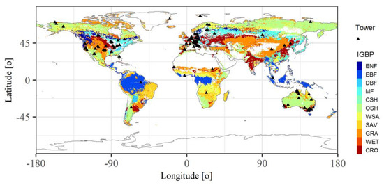
Figure 1.
Geographical distribution of flux towers overlaid onto the 2005 Moderate Resolution Imaging Spectroradiometer (MODIS) International Geosphere–Biosphere Programme (IGBP) land cover map at a 0.5° × 0.5° resolution. ENF: evergreen needleleaf forests; EBF: evergreen broadleaf forests; DBF: deciduous broadleaf forests; MF: mixed forests; CSH: closed shrublands; OSH: open shrublands; WSA: woody savanna; SAV: savanna; GRA: grasslands; WET: permanent wetlands; CRO: croplands.
2.2. Vegetation and Climate Datasets
Previous studies have reported that vegetation change is a primary driver of surface energy fluxes variations, especially for the LE in which more than 50% of it could be explained by vegetation greening [34,35]. Leaf area index has been widely used as an indicator to monitor vegetation dynamics for its advantage of providing quantitative information of vegetation coverage, productivity and greenness, and is also adopted by this study. Given the facts that uncertainties exist in different LAI products projected by different algorithms, three different satellite-derived LAI products were considered in the RF models to predict global surface fluxes. The Global Inventory Modeling and Mapping Studies (GIMMS) LAI3g dataset was constructed by the Artificial Neural Network (ANN) model from GIMMIS Normalized difference vegetation index (NDVI3g) dataset [36]. The ANN model was established by training GIMMIS NDVI3g and MODIS LAI datasets for the overlapping period 2000–2009. The Long-term Global Mapping (GLOBMAP) LAI dataset was generated by combing both MODIS LAI and Advanced Very High Resolution Radiometer (AVHRR) LAI [37]. The pixel-by-pixel relationship was established first based on MODIS LAI and GIMMIS NDVI during the overlapped period (2000–2006), and was used to derive historical AVHRR LAI during 1982–2000 from GIMMIS NDVI. GLOBMAP and GIMMIS LAI datasets have the same temporal resolution of half month, but their spatial resolutions are 1/12 degree and 8 km, respectively. The Global LAnd Surface Satellite (GLASS) LAI was constructed based on general regression neural networks, which are trained with the fused MODIS and CYCLOPES LAI (from SPOT/VEGETATION) products and the AVHRR reflectance data [38]. The spatial resolution is 0.05 degree with 8-day time step spanning from 1982–2016. Besides, since LAI observations are not available in eddy covariance sites, the MODIS LAI (MOD15A2H) was used to train RF models because of its high spatial resolution of 500 m. The best pixels were extracted based on its associated QC flags, and finally were aggregated into monthly data from 8-day step to match with observed surface energy fluxes. The MODIS IGBP land cover map (MCD12C1) in 2005 was obtained from the land processes distributed active archive center (LP DAAC). The product has a spatial resolution of 0.05°. The 0.5° spatial resolution map was produced by the dominant land cover types in our global surface energy flux estimations.
The latest version of global climate forcing datasets (CRUNCEP V7) were obtained from Research Data Archive at the National Center for Atmospheric Research [39]. These datasets were constructed by combing two existing datasets: the Climate Research Unit (CRU) monthly data and the reanalysis data developed by National Centers for Environmental Prediction (NCEP), and were initially constructed to drive land surface models by their highly temporal (6-h) and spatial (0.5 degree) resolutions. Global monthly mean CO2 concentration data were obtained from The Global Monitoring Division of NOAA/Earth System Research Laboratory, which is available from 1980 to date [40].
Atmospheric vapor pressure deficit (VPD), defined as the difference between saturate vapor pressure (SVP) and actual vapor pressure (AVP) for a given temperature, is also a potential factor in controlling surface energy fluxes, especially for the LE, by determining air vapor holding capacity and vapor exchange between vegetation and atmosphere through controlling stomatal closure [41]. It was calculated from other existing climate factors from CRUNCEP datasets based on the following equations [42]:
where fw is an enhanced factor in moist air and Ps is the surface pressure.
2.3. Random Forest Model
The random forest method (RF) was used to reconstruct the surface fluxes during 1982–2016. RF is a tree-based ensemble approach and the predictions are averaged by all decision trees, which can be used for both classification and regression purposes [43]. Each decision tree was built independently by a bootstrap sample of the data set, randomly generated from the predictor variable values [44]. Each node of the decision tree was based on one characteristic (i.e., predictor variable) and the final outputs depend on the majority votes. This allows RF to avoid collinearity between predictor variables. RF has been widely used in agricultural, ecological and meteorological studies, and has demonstrated to be a robust method to reconstruct surface parameters [3,30]. Seven predictor variables, SR, PRE, TEM, wind, LAI, VPD and CO2 are selected to build RF models for both LE and H, which have proven to play a significant role in regulating surface energy partitioning [3,45,46,47]. RF was implemented by package “randomForest” in R language [41]. ‘mtry’ and ‘ntree’ are two parameters needed to be adjusted in RF. ‘mtry’ represents the number of randomly chosen predictor variables in each node of one decision tree and predefined as one third of total number of predictor variable, while ntree represents the number of total decision trees and predefined as 500 in RF. Here, ‘ntree’ is adjusted as 1000 based on the fact that the outputs tend to be stable. The parameter ‘mtry’ was not tuned because the model performance changed slightly compared to the default ‘mtry’.
2.4. Morris Sensitivity Method
The Morris sensitivity analysis is an effective method to filter out important factors in models expressed mathematically [48]. The importance ranking of input factors are determined by both the mean (μi) and standard deviation (σi) of the elementary effects attributable to each input. Before implementation, all the inputs are scaled to [0, 1], and the elementary effects (Ei) of parameter xi are expressed as:
where f is the computational model referred to as RF in this study and Δ is the step size of input parameter xi; Δ is equal to j/2(j − 1) [49], and j is the sampling levels that is predefined. The starting parameter is randomly selected and varies by Δ, while other parameters are fixed. Then the second parameter is selected and varies again by Δ, until all the parameters are implemented. This is repeated r times (i.e., r trajectories). Therefore, the mean elementary effect of parameter xi is expressed as:
The standard deviation of elementary effects of parameter xi is expressed as:
where μi represents the overall effects of xi on model output and σi means the interactions/non-linearities with other parameters.
To determine the important parameters, a measure of importance for parameter xi (βi) is suggested by Lu et al. [50], which is calculated by considering both μi and σi,
where β0 is a threshold above which that parameter is considered to be important and is suggested as 0.85 by the study from Lu et al. [50]; is the standard deviation of of all parameters. Thus, the important ranking of input parameters can be obtained according to βi values.
2.5. Experimental Design
Two types of experimental simulations were designed to extract the relative contributions of individual factors to the surface energy fluxes. In the first simulation, all the drivers, including vegetation and climate predictor variables, were set to vary during 1982–2016, which is defined as the total effects (Stotal). In the second type of simulations, only one driver (SLAI, STEM, SPRE, SVPD, SSW, Sco2 and SWind) was kept at the initial state (1982), while the remaining drivers were set to vary with time. The difference between these two types of simulations was defined as the contribution of the corresponding factor to the changes in surface energy fluxes. For example, the contribution of LAI to LE variation during 1982–2016 was calculated as follows,
This equation was also applied to H and other factors.
2.6. Model Evaluation
We used coefficient of determination (R2), root mean square error (RMSE) and mean bias error (MBE) to assess the agreement between the predictions and the observations. The equations [51,52] are given as follows,
where xi and yi are the observed and modeled values, respectively; n is the number of observed and modeled values; is the mean value of observations. A value of one for the R2 indicates a perfect match, and zero indicates no agreement at all. The smaller the value of RMSE and MBE, the better the agreement between the observations and simulations.
The k-fold cross validation method [53] was applied to assess the capability and stability of RF to estimate surface energy fluxes. Particularly, the original dataset is randomly partitioned into k equal sized groups. Then, one of the groups was chosen for testing the model, and the remaining k−1 groups were used as training data. This cross-validation process is then repeated k times, until each of the groups was used once as the validation data. The value of k was fixed as 10, as it is commonly used [54].
3. Results
3.1. Evaluation of the Capability of RF in Predicting LE and H
Based on the RF models that were constructed 10 times for each of the 10 PFTs by the k-fold cross validation method, the performance was assessed by R2, RMSE and MBE in Figure 2. For the LE, the mean values of R2 range from 0.66 to 0.89, with the maximum value in WSA and the minimum value in MF. The most unstable performance of RF model occurs in MF, whose R2 values fluctuate from 0.34 to 0.89. Correspondingly, the largest fluctuation in RMSE was present in MF, with the values ranging from 10.15 W/m2 to 31.40 W/m2. The mean values of RMSE range from 12.20 W/m2 in SH to 21.94 W/m2 in DBF. In contrast, the MBE are relatively stable, with the mean values fluctuating from 0.23 W/m2 to 0.40 W/m2 across 10 PFTs.
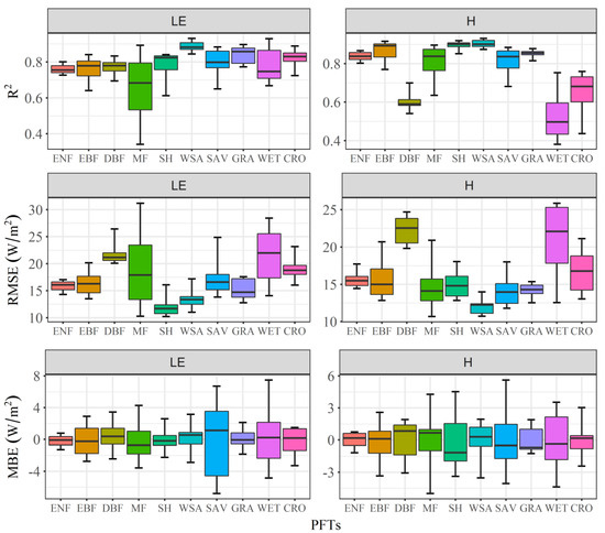
Figure 2.
Random forest (RF) performance for simulating latent (LE) and sensible (H) heat fluxes as indicated by coefficient of determination (R2), root mean square error (RMSE) and mean bias error (MBE) across multiple plant functional types (PFTs). The black line within the box indicates the mean values of statistical metrics. Box boundaries indicate the 30th and 70th percentiles, whiskers below and above the box indicate the minimum and maximum values. ENF: evergreen needleleaf forests; EBF: evergreen broadleaf forests; DBF: deciduous broadleaf forests; MF: mixed forests; SH: board shrublands including both closed and open shrublands; WSA: woody savanna; SAV: savanna; GRA: grasslands; WET: permanent wetlands; CRO: croplands.
For the H, the mean R2 values were distributed between 0.53 in WET and 0.90 in WSA. The explanatory ability of RF in predicting H is stronger in ENF, EBF, MF, SH, WSA, SAV and GRA with the R2 values higher than 0.8. However, the explanatory ability of RF is relatively weak in DBF, WET and CRO whose R2 values are lower than 0.70. The higher R2 values are normally followed by the lower RMSE values. For example, the mean values of RMSE in DBF, WET and CRO are 22.35, 20.84 and 16.75 W/m2 respectively, which are higher than other PFTs. The lowest mean RMSE is 12.05 W/m2 presented in WSA. Similar to the LE, the MBE is also relatively stable for the H, with the mean values fluctuating from 0.23 W/m2 in SH to 0.22 W/m2 in MF. These statistic metrics suggest an acceptable forecasting capability of RF in predicting LE and H.
3.2. Important Predictor Variables in Predicting LE and H
The LE and H are considerably constrained by predictor variables. The ranking of importance in these variables were identified by the Morris sensitivity method in this study. Guided by previous analyses, the RF models with the lowest RMSE for each PFT were chosen for the following analyses. As shown in Figure A1, taking GRA as an example, the elementary effects of predictor variables as quantified by β values fluctuated with the number of trajectories (r). However, these fluctuations become small and stable when the r reaches 2000 for both LE and H, which is sufficient for screening out the importance of predictor variables. As shown in Figure 3, the identified important variables are different for LE and H, and are also different across different PFTs. For the LE, specifically, the SR, TEM, LAI are the sensitive factors and are common to all 10 PFTs. VPD is identified as a sensitive one for most PFTs except for SH. PRE is considered to have limited effects in the forests, such as in EBF, ENF, DBF and in MF. For the H, the SR is the most important variable for all PFTs whose β values are higher than any other factors. Furthermore, VPD is identified as a sensitive factor for most PFTs, except for ENF and EBF. Except for the DBF, WET and CRO, the numbers of sensitive factors for LE are higher than the sensitive numbers for the H. These results suggest that the LE are more sensitive to ambient conditions and difficult to be captured than the H as it is constrained by more variables. The SR is the only factor that influences both LE and H for all 10 PFTs, suggesting that H and LE are coupled strongly by SR at PFT scale.
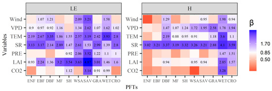
Figure 3.
Morris sensitivity analysis for latent (LE) and sensible (H) heat fluxes across different plant functional types (PFTs). ENF: evergreen needleleaf forests; EBF: evergreen broadleaf forests; DBF: deciduous broadleaf forests; MF: mixed forests; SH: board shrublands including both closed and open shrublands; WSA: woody savanna; SAV: savanna; GRA: grasslands; WET: permanent wetlands; CRO: croplands; LAI: leaf area index; PRE: precipitation; SR: solar radiation; TEM: temperature; VPD: vapor pressure deficit.
3.3. Inter-Annual Variations in LE and H
Temporal and spatial patterns of global LE and H between 1982 and 2016 were estimated by RF models which were driven by gridded climatic datasets and satellite-based LAI (Figure 4). The results show a mean value of 42.65 ± 1.54 W/m2 for LE and 36.26 ± 0.44 W/m2 for H during 19822016, respectively. All of these LE estimations by three different LAI products show a consistently significant increasing trend with a speed of 0.054~0.073 W/m2 per year. Nevertheless, the magnitude between them differs, with the largest estimation from GLASS LAI (i.e., 44.01 W/m2 during 19822016), followed by GIMMIS (i.e., 42.10 W/m2 during 19822016) and GLOBMAP LAI (i.e., 41.83 W/m2 during 19822016). In contrast, all of the H estimations show a decreasing trend with a speed of 0.005~0.013 W/m2 per year, but only the GLASS estimation is significant (p < 0.05). The discrepancy between the three estimations is relatively smaller compared to LE, and their mean values during 19822016 distributed between 36.02 W/m2 from GLASS LAI and 36.52 W/m2 from GIMMIS LAI. Spatially, most parts of the Earth experienced an increasing trend in LE (54.4% grids), and 34.5% grids are significant (Figure 4), distributed in mid- and high-latitudes of northern hemisphere with hotspots in northern parts of South America, Western Europe and southern parts of Africa. About 19% grids underwent a significantly decreasing trend in LE and mainly occurred in middle-latitudes of northern hemisphere. For the H, 37.5% of the Earth was dominated by a significantly decreasing trend, with hotspot in eastern parts of Asia. Meanwhile, 34.2% grids presented a significantly increasing trend.
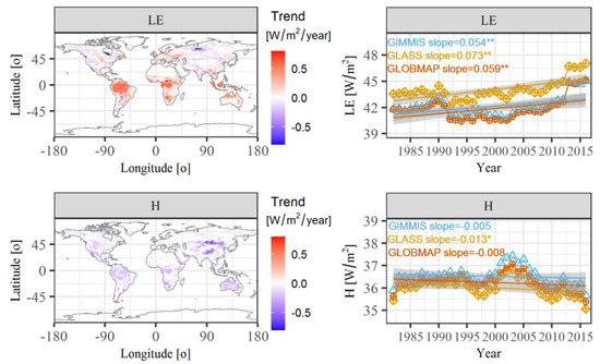
Figure 4.
Temporal and spatial trends of latent (LE) and sensible (H) heat fluxes during 1982–2016. The spatial maps of long-term trends are averaged by outputs of RF models that are driven by three different LAI datasets. Only the cells that are statistically significant at p < 0.05 level are shown. * and ** indicate the significance levels at 0.05 and 0.01, respectively.
3.4. Contributions of Individual Factors to H and LE Variations
Almost all the predictor variables show a significant increasing trend during 1982–2016, except for the wind (Figure A2). Evidently, the largest increasing speed was presented in CO2, from 340 ppm in 1982 to more than 400 ppm in 2016, and increased by ~17%. LAI, TEM and VPD also show a strong increasing trend, as indicated by R2 ranging from 0.74 to 0.89. However, the SR and PRE showed a slightly increasing trend, but still significantly (p < 0.05). Any changes in these variables can lead to the changes in the surface energy fluxes and further exert influences on surface energy balance. Here, the relative contributions of such individual factor variations to H and LE changes were quantified by conducting single factor experiments. The spatial patterns show that the elevated CO2 concentration played a profound impact on the changes of LE (Figure 5). The elevated CO2 concentration contributed an increase in LE in the southern hemisphere and some parts in the mid-latitudes of northern hemisphere, such as eastern parts of Asia and western parts of Europe, while the decrease of LE caused by CO2 mainly occurred in high-latitudes of northern hemisphere and some arid regions, such as middle parts of Asia and west parts of North America. Nearly 70.5% of the Earth experienced an increase of LE under the effect of LAI increase. Meanwhile, 64.4% of the Earth undergone an increase of LE caused by the TEM rise. The areas that experienced an increase or a decrease in LE caused by PRE changes are comparable (51% vs. 49%). VPD, SR and wind exerted limited impacts on the LE. Our results show that the increased CO2 contributed most to the decrease of LE among these factors with a value of 0.61 W/m2 during 19822016, followed by the VPD and wind with the values of 0.032 W/m2 and 0.028 W/m2, respectively. On the contrary, the increase of LAI causes the most increase in LE with a value of 0.57 W/m2, followed by TEM, PRE and SR with the values of 0.26 W/m2, 0.08 W/m2 and 0.03 W/m2, respectively.
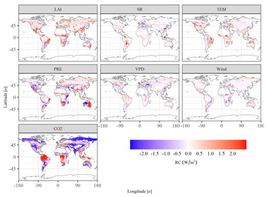
Figure 5.
The spatial map of relative contributions (RC) of different influencing factors to latent heat fluxes (LE) during 1982–2016. LAI: leaf area index; PRE: precipitation; SR: solar radiation; TEM: temperature; VPD: vapor pressure deficit.
Contrast to the LE, the elevated CO2 concentration contributed a decrease in H in the southern hemisphere and some parts in the mid-latitudes of northern hemisphere and the increase of H caused by CO2 mainly occurred in high-latitudes of northern hemisphere (Figure 6). There are 84.9% and 61.2% regions experiencing a decrease of H caused by TEM and LAI, respectively. Overall, the increased CO2 contributed most to the increase of H among these factors with a value of 0.57 W/m2 during 1982–2016 (Figure 7). Conversely, TEM contributed most the decrease of H with a value of 0.34 W/m2, followed by the LAI with a value of 0.24 W/m2. Furthermore, wind, SR, VPD and PRE caused marginal changes of H with the values of 0.01, 0.03, 0.07 and 0.08 W/m2, respectively.
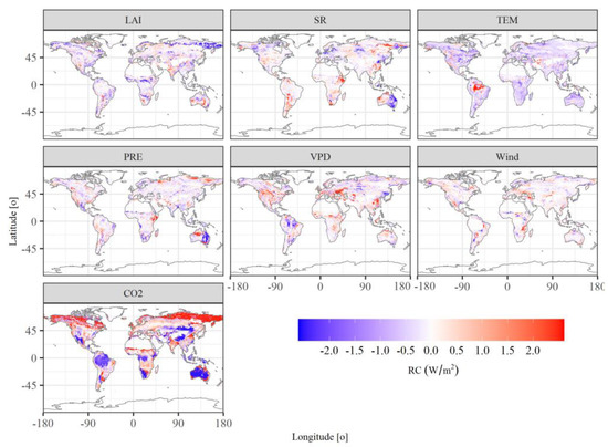
Figure 6.
The spatial map of relative contributions (RC) of different influencing factors to sensible heat fluxes (H) during 1982–2016. LAI: leaf area index; PRE: precipitation; SR: solar radiation; TEM: temperature; VPD: vapor pressure deficit.
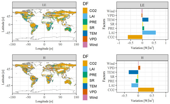
Figure 7.
The relative contributions of different influencing factors to variations of latent (LE) and sensible (H) heat fluxes. The spatial maps indicate the dominant factors (DF) that contribute most to the variation of LE and H during 1982–2016. LAI: leaf area index; PRE: precipitation; SR: solar radiation; TEM: temperature; VPD: vapor pressure deficit.
By comparing the effects of different factors, we further analyzed the spatial pattern of the dominant controls. The changes of both LE and H dominated by elevated CO2 concentration occurred in most parts of the Earth, which account for 54.8% and 52.0%, respectively (Figure 7). For LE, the LAI controls were mainly distributed in eastern parts of China and Brazil and southeastern parts of North America. Most regions of Australia and southeastern parts of Africa were dominated by PRE. For the H, only some eastern parts of South America and middle parts of Africa were dominated by LAI.
4. Discussion
4.1. Comparisons with Previous Studies
The understanding of global-scale surface energy partitioning is still a challenging problem due to the complex interactions between the atmosphere and the surface as well as their spatial inhomogeneity. Machine learning methods has greatly enhanced our ability to predict and monitor the surface energy fluxes variations, by avoiding describing complicated biophysical or biochemical mechanisms. Fortunately, the established RF models by feeding site-observed monthly climatic and vegetation factors have a high potential in estimating the LE and H, which overall accounted for 0.66~0.89 variations for LE and 0.53~0.90 for H, respectively. Our estimations show a highly comparable performance to other studies. The detailed comparisons between this study and other products are listed in Table 1. For example, based on a common period between 2001 and 2010, we estimated a mean value of 42.27 ± 1.25 W/m2 for LE and 36.52 ± 0.52 W/m2 for H, respectively, which is close to 44.48 ± 0.16 W/m2 for LE and 37.08 ± 0.33 W/m2 for H estimated by Jung et al. [29], which is averaged by multiple machine learning methods. However, these estimations are inconsistent with our previous study which used a process-based land surface model (i.e., Common Land Model (CoLM)) [55]. The LE is higher than CoLM estimate with a value of 40.37 ± 1.21 W/m2, but the H is lower than CoLM-based estimate 37.14 ± 1.11 W/m2. The differences may come from a systematical underestimation of albedo by CoLM, which affect the net radiation received by the surface and further exert an influence on the energy partitioning between LE and H. Forzieri et al. [45] also reported a systematic model underestimation of LE by assessing 10 state-of-the-art LSMs simulations. They reported that the overestimation of the sensitivity to CO2 and the underestimation of the biophysical response of ecosystems to changes in water availability in current LSMs may lead to the underestimations of LE in LSMs. Besides, we further compared LE with three other ET products derived from Global Land Evaporation Amsterdam Model (GLEAM), MODIS improved ET algorithm and Model tree ensemble (MTE) methods by combining with latent heat of vaporization (λ = 2.45 MJ kg−1). These authors estimated a mean annual LE of 39.54 ± 0.51, 38.51 ± 0.50 and 38.84 ± 0.40 W/m2 for GLEAM, MODIS and MTE, respectively, which are lower than our estimates. The comparisons above suggest a large uncertainty exists in current widely used LE and H products. Therefore, intercomparisons of various datasets estimated by different methods are needed for a better understanding of surface energy partitioning in the future studies. And this study provides a valuable contribution to the surface energy flux prediction.

Table 1.
Comparisons of latent (LE) and sensible (H) heat fluxes between our study and past studies. The symbol ‘×’ means the data are not available.
4.2. The Sensitivity of Predictor Variables to H and LE Variations
Assessing the sensitivity of individual factors to predict the LE and H will be helpful to identify which one among the several factors is important in determining H and LE changes. This provides a feasible and efficient way to monitor LE or H changes by focusing on limited variables. The important factors identified by Morris sensitivity method differ in determining variations of LE and H. We found that SR, LAI and TEM are important in LE, while SR is important in H across 10 PFTs. The important factor SR is common to both LE and H and to all 10 PFTs. This is because SR controls energy supply for both LE and H, and the magnitudes of their change are directly affected by SR. Another possible reason may come from the established RF models which are trained by monthly observation. Most of the stations (115 out of 152) are located in temperate regions with periodically or seasonally dynamic values that may give rise to the high sensitivity to SR.
PRE and TEM are also two important climatic factors which affect LE, because they regulate moisture supply and moisture holding capacity of the air [59,60]. However, the forests are not sensitive to the PRE compared to other PFTs. PRE regulates moisture supply through governing the soil water content [61], which becomes more significant in arid/semi-arid ecosystems where the precipitation is the primary channel to provide water resource [56]. This is also demonstrated by our results when the sensitivity is projected into different PFTs. The higher sensitivities occurred in relatively arid ecosystems such as in WSA and SAV where the β values are 2.06 and 3.53, respectively. While lower sensitivities are mainly distributed in relatively humid ecosystems, such as in forests (i.e., ENF, ENF, DBF and MF in this study), where the β values are lower than 0.85. LAI is another sensitive factor that could exert influence on both LE and H, especially for LE. It is reasonable to say that LAI impacts the exchange of energy fluxes between the land and the atmosphere through albedo, because a larger LAI is associated with a lower albedo, and more energy will be absorbed by the surface [62]. Besides, LAI is a key representative of leaf area which is expected to control the transpiration area [63], and thus, to affect the LE variations. CO2 was expected to exert a critical impact on the the surface energy fluxes because of its greenhouse effect by enhancement of downward long-wave radiation, and also because its elevated concentration would lead to a closure of the stomatal apertures, leading to a decrease of transpiration [64]. However, its importance was not screened out for LE on forests, WSA and CRO, but only occurs in SH, SAV, GRA and WET. The sensitivity of surface energy partitioning to climatic and vegetation factors are divergent with respect to different PFT-scales. This finding is supported by Valayamkunnath et al. [65] which suggested that surface energy partitioning differs among different ecosystems due to heterogeneity in available energy, soil moisture conditions and vegetation characteristics. Beside the factors analyzed in this study, other factors are also reported to have an important role in influencing surface energy fluxes changes. For example, Yao et al. [33] found that snow cover, soil content and soil texture have a large influence on the surface energy balance in high-elevation areas of the Tibet plateau. Therefore, more localized and in-depth analyses are required in the future.
4.3. Inter-Annual Trends of LE and H and Their Dominant Factors
Our findings show that a contrasting trend was presented for LE and H: a positive trend in LE (0.054~0.073 W/m2 per year) and a negative trend in H (0.005~0.013 W/m2 per year) during 1982–2016 and these contrasting trends are largely controlled by the variations of CO2. These findings are consistent and comparable with previous studies using statistical algorithm, or process-based biophysical models [66,67]. For example, Zhang et al. [35] used a remote-sensing-driven ET algorithm and found a significant upward global trend of LE at a rate of 0.068 W/m2 per year. Zeng et al. [34] also found a positive trend of LE at a rate of 0.059 W/m2 per year during 1982–2011 by using an ensemble of several physics-based formula reconstructions. All these studies show that the positive trend of LE is driven by the global greening (indicated by NDVI or LAI) and their growth rates also fall within our estimates. However, our findings seem to be inconsistent with FLUXCOM product [29], which shows a much lower upward global trend in LE at a rate of 0.004 W/m2 per year but not significantly (p > 0.05), and also an opposite trend in H at a rate of 0.01 W/m2 per year. We note that the discrepancy between our findings and their results may come from the predictor variables. The effects of CO2 were not taken into account in their estimates but were in our established RF models. This finding suggests that CO2 is the most influencing factor in determining surface energy partitioning. Zhang et al. [66] quantified the contributions of changes in CO2 to transpiration and evaporation during 1982–2012 using Community Atmosphere–Biosphere Land Exchange model (CABLE). They reported that the increasing CO2 concentrations reduced transpiration 0.17 mm per year and increased evaporation by 0.04 mm per year, and hence reduced LE by approximate 0.01 W/m2 per year during 1981–2012 which is comparable to 0.017 W/m2 per year in our study. Therefore, CO2 are highly recommended to be investigated in future researches given its important role in affecting surface energy fluxes.
5. Conclusions
The dramatic climate change and wide spread of global greening in recent past decades are expected to alter the surface energy partitioning. However, large uncertainties exist in predicting both LE and H, as reported in previous studies based on statistical methods, physical-based algorithms or process-based models. The machine learning method of RF was assessed to predict LE and H and their long-term trends and their dominant factors were analyzed. From this study, we conclude that:
- (1)
- The established RF models in this study have a high potential in predicting and monitoring the surface energy flux variations. However, their predicted performance is different among PFTs. The variations of LE can be explained from 0.66 to 0.89, while the H can be explained from 0.53 to 0.90 across 10 PFTs, indicated by R2. Meanwhile, the RMSE ranges from 12.20 W/m2 to 21.94 W/m2 for the LE and from 12.05 W/m2 to 22.34 W/m2 for the H at a monthly scale, respectively.
- (2)
- The important influencing factors are different in LE and H based on Morris sensitive method. Particularly, The SR, LAI and TEM are important factors in LE, while SR is important in H across 10 PFTs in this study. Besides, the important factors are divergent with respect to PFT-level.
- (3)
- A contrasting trend was presented for LE and H: a positive trend in LE with a rate of 0.054~0.073 W/m2 per year and a negative trend in H with a rate of 0.005~0.013 W/m2 per year during 1982–2016 and these contrasting trends are largely controlled by the variation of CO2. Our study emphasizes the need to better account for the influence of elevated CO2 in energy partitioning to improve surface energy fluxes estimations in future studies.
Author Contributions
Conceptualization, X.Y.; methodology, X.Y.; validation, X.Y.; formal analysis, X.X., F.U.O.; writing—original draft preparation, X.X., F.U.O.; writing—review and editing, X.Y., F.U.O.; visualization, P.D.M. and A.K.; supervision, P.D.M.; funding acquisition, X.Y., F.U.O., P.D.M. All authors have read and agreed to the published version of the manuscript.
Funding
This work was financially supported by the Research Foundation – Flanders (FWO) (Grant No. 12T1419N), the Chinese Academy of Sciences President’s International Fellowship Initiative (PIFI, Grant No. 2017VCA0002) and the Chinese Academy of Sciences-the World Academy of Sciences (CAS-TWAS) President’s Fellowship Programme (2017A8010210001).
Acknowledgments
We thank the global FLUXNET community who provides the global flux data.
Conflicts of Interest
The authors declare no conflict of interest.
Appendix A
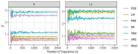
Figure A1.
Variations of the elementary effects as quantified by β values with number of trajectories based on Morris sensitive method. LAI: leaf area index; PRE: precipitation; SR: solar radiation; TEM: temperature; VPD: vapor pressure deficit.
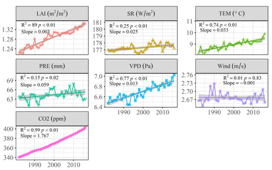
Figure A2.
Long-term trend of different climate and vegetation factors. LAI: leaf area index; PRE: precipitation; SR: solar radiation; TEM: temperature; VPD: vapor pressure deficit.
References
- Wilson, K.B.; Baldocchi, D.D.; Aubinet, M.; Berbigier, P.; Bernhofer, C.; Dolman, H.; Falge, E.; Field, C.; Goldstein, A.; Granier, A. Energy partitioning between latent and sensible heat flux during the warm season at FLUXNET sites. Water Resour. Res. 2002, 38, 30–31. [Google Scholar] [CrossRef]
- Li, Y.; Zhao, M.; Motesharrei, S.; Mu, Q.; Kalnay, E.; Li, S. Local cooling and warming effects of forests based on satellite observations. Nat. Commun. 2015, 6, 1–8. [Google Scholar] [CrossRef] [PubMed]
- Yuan, W.; Zheng, Y.; Piao, S.; Ciais, P.; Lombardozzi, D.; Wang, Y.; Ryu, Y.; Chen, G.; Dong, W.; Hu, Z. Increased atmospheric vapor pressure deficit reduces global vegetation growth. Sci. Adv. 2019, 5, eaax1396. [Google Scholar] [CrossRef] [PubMed]
- Huang, L.; Zhai, J.; Liu, J.; Sun, C. The moderating or amplifying biophysical effects of afforestation on co2-induced cooling depend on the local background climate regimes in china. Agric. For. Meteorol. 2018, 260, 193–203. [Google Scholar] [CrossRef]
- Rigden, A.J.; Li, D. Attribution of surface temperature anomalies induced by land use and land cover changes. Geophys. Res. Lett. 2017, 44, 6814–6822. [Google Scholar] [CrossRef]
- Siler, N.; Roe, G.H.; Armour, K.C.; Feldl, N. Revisiting the surface-energy-flux perspective on the sensitivity of global precipitation to climate change. Clim. Dynam. 2019, 52, 3983–3995. [Google Scholar] [CrossRef]
- Bala, G.; Caldeira, K.; Wickett, M.; Phillips, T.; Lobell, D.; Delire, C.; Mirin, A. Combined climate and carbon-cycle effects of large-scale deforestation. Proc. Natl. Acad. Sci. USA 2007, 104, 6550–6555. [Google Scholar] [CrossRef]
- Bathiany, S.; Claussen, M.; Brovkin, V.; Raddatz, T.; Gayler, V. Combined biogeophysical and biogeochemical effects of large-scale forest cover changes in the MPI earth system model. Biogeosciences 2010, 7, 1383–1399. [Google Scholar] [CrossRef]
- Ukkola, A.M.; Prentice, I.C.; Keenan, T.F.; Van Dijk, A.I.; Viney, N.R.; Myneni, R.B.; Bi, J. Reduced streamflow in water-stressed climates consistent with CO 2 effects on vegetation. Nat. Clim. Chang. 2016, 6, 75–78. [Google Scholar] [CrossRef]
- Feng, X.; Fu, B.; Piao, S.; Wang, S.; Ciais, P.; Zeng, Z.; Lü, Y.; Zeng, Y.; Li, Y.; Jiang, X. Revegetation in China’s Loess Plateau is approaching sustainable water resource limits. Nat. Clim. Chang. 2016, 6, 1019–1022. [Google Scholar] [CrossRef]
- Peng, J.; Kharbouche, S.; Muller, J.-P.; Danne, O.; Blessing, S.; Giering, R.; Gobron, N.; Ludwig, R.; Müller, B.; Leng, G. Influences of leaf area index and albedo on estimating energy fluxes with HOLAPS framework. J. Hydrol. 2020, 580, 124245. [Google Scholar] [CrossRef]
- Pastorello, G.; Trotta, C.; Canfora, E.; Chu, H.; Christianson, D.; Cheah, Y.-W.; Poindexter, C.; Chen, J.; Elbashandy, A.; Humphrey, M. The FLUXNET2015 dataset and the ONEFlux processing pipeline for eddy covariance data. Sci. Data 2020, 7, 1–27. [Google Scholar] [CrossRef] [PubMed]
- Hao, Y.; Baik, J.; Choi, M. Developing a soil water index-based Priestley–Taylor algorithm for estimating evapotranspiration over East Asia and Australia. Agric. For. Meteorol. 2019, 279, 107760. [Google Scholar] [CrossRef]
- Wang, K.; Wang, P.; Li, Z.; Cribb, M.; Sparrow, M. A simple method to estimate actual evapotranspiration from a combination of net radiation, vegetation index, and temperature. J. Geophys. Res. Atmos. 2007, 112, D15107. [Google Scholar] [CrossRef]
- Yao, Y.; Liang, S.; Zhao, S.; Zhang, Y.; Qin, Q.; Cheng, J.; Jia, K.; Xie, X.; Zhang, N.; Liu, M. Validation and application of the modified satellite-based Priestley-Taylor algorithm for mapping terrestrial evapotranspiration. Remote Sens. 2014, 6, 880–904. [Google Scholar] [CrossRef]
- Jacob, F.; Olioso, A.; Gu, X.F.; Su, Z.; Seguin, B. Mapping surface fluxes using airborne visible, near infrared, thermal infrared remote sensing data and a spatialized surface energy balance model. Agronomie 2002, 22, 669–680. [Google Scholar] [CrossRef]
- Su, Z. The Surface Energy Balance System (SEBS) for estimation of turbulent heat fluxes. Hydrol. Earth Syst. Sci. 2002, 6, 85–99. [Google Scholar] [CrossRef]
- Jimenez, C.; Prigent, C.; Mueller, B.; Seneviratne, S.I.; McCabe, M.; Wood, E.F.; Rossow, W.; Balsamo, G.; Betts, A.; Dirmeyer, P. Global intercomparison of 12 land surface heat flux estimates. J. Geophys. Res. Atmos. 2011, 116, D02102. [Google Scholar] [CrossRef]
- Dai, Y.; Zeng, X.; Dickinson, R.E.; Baker, I.; Bonan, G.B.; Bosilovich, M.G.; Denning, A.S.; Dirmeyer, P.A.; Houser, P.R.; Niu, G. The common land model. Bull. Am. Meteorol. Soc. 2003, 84, 1013–1024. [Google Scholar] [CrossRef]
- Bonan, G.B. Land Surface Model (LSM version 1.0) for Ecological, Hydrological, and Atmospheric Studies: Technical Description and Users Guide; Technical Note; National Center for Atmospheric Research: Boulder, CO, USA, 1996. [Google Scholar]
- Stöckli, R.; Lawrence, D.; Niu, G.Y.; Oleson, K.; Thornton, P.E.; Yang, Z.L.; Bonan, G.; Denning, A.; Running, S.W. Use of FLUXNET in the Community Land Model development. J. Geophys. Res. Biogeosci. 2008, 113, G01025. [Google Scholar] [CrossRef]
- Bakketun, Å. Data Assimilation of Satellite Soil Moisture Retrievals in the Land Surface Model SURFEX. Master’s Thesis, University of Oslo, Oslo, Norway, 2017. [Google Scholar]
- Li, J.; Duan, Q.; Gong, W.; Ye, A.; Dai, Y.; Miao, C.; Di, Z.; Tong, C.; Sun, Y. Assessing parameter importance of the Common Land Model based on qualitative and quantitative sensitivity analysis. Hydrol. Earth Syst. Sci. 2013, 17, 3279. [Google Scholar] [CrossRef]
- Li, Y.; Li, L.; Dong, J.; Bai, J.; Yuan, X.; Song, S.; Zhao, H.; Chen, X.; Li, Y. Process refinement contributed more than parameter optimization to improve the CoLM’s performance in simulating the carbon and water fluxes in a grassland. Agric. For. Meteorol. 2020, 291, 108067. [Google Scholar] [CrossRef]
- Khanna, J.; Medvigy, D. Strong control of surface roughness variations on the simulated dry season regional atmospheric response to contemporary deforestation in Rondônia, Brazil. J. Geophys. Res. Atmos. 2014, 119, 13067–13078. [Google Scholar] [CrossRef]
- Chen, Y.; Yang, K.; He, J.; Qin, J.; Shi, J.; Du, J.; He, Q. Improving land surface temperature modeling for dry land of China. J. Geophys. Res. Atmos. 2011, 116, D20104. [Google Scholar] [CrossRef]
- Freitas, S.C.; Trigo, I.F.; Bioucas-Dias, J.M.; Gottsche, F.-M. Quantifying the uncertainty of land surface temperature retrievals from SEVIRI/Meteosat. IEEE T Geosci. Remote 2009, 48, 523–534. [Google Scholar] [CrossRef]
- Hua, W.; Chen, H.; Sun, S. Uncertainty in land surface temperature simulation over China by CMIP3/CMIP5 models. Theor. Appl. Clim. 2014, 117, 463–474. [Google Scholar] [CrossRef]
- Jung, M.; Koirala, S.; Weber, U.; Ichii, K.; Gans, F.; Camps-Valls, G.; Papale, D.; Schwalm, C.; Tramontana, G.; Reichstein, M. The FLUXCOM ensemble of global land-atmosphere energy fluxes. Sci. Data 2019, 6, 1–14. [Google Scholar] [CrossRef]
- Wang, B.; Feng, P.; Waters, C.; Cleverly, J.; Li Liu, D.; Yu, Q. Quantifying the impacts of pre-occurred ENSO signals on wheat yield variation using machine learning in Australia. Agric. For. Meteorol. 2020, 291, 108043. [Google Scholar] [CrossRef]
- Meyer, H.; Reudenbach, C.; Wöllauer, S.; Nauss, T. Importance of spatial predictor variable selection in machine learning applications–Moving from data reproduction to spatial prediction. Ecol. Model. 2019, 411, 108815. [Google Scholar] [CrossRef]
- Xu, T.; Guo, Z.; Liu, S.; He, X.; Meng, Y.; Xu, Z.; Xia, Y.; Xiao, J.; Zhang, Y.; Ma, Y. Evaluating different machine learning methods for upscaling evapotranspiration from flux towers to the regional scale. J. Geophys. Res. Atmos. 2018, 123, 8674–8690. [Google Scholar] [CrossRef]
- Yao, J.; Gu, L.; Yang, C.; Chen, H.; Wang, J.; Ding, Y.; Li, R.; Zhao, L.; Xiao, Y.; Qiao, Y. Estimation of surface energy fluxes in the permafrost region of the Tibetan Plateau based on in situ measurements and the surface energy balance system model. Int. J. Climatol. 2020, 40, 5783–5800. [Google Scholar] [CrossRef]
- Zeng, Z.; Peng, L.; Piao, S. Response of terrestrial evapotranspiration to Earth’s greening. Curr. Opin. Environ. Sustain. 2018, 33, 9–25. [Google Scholar] [CrossRef]
- Zhang, K.; Kimball, J.S.; Nemani, R.R.; Running, S.W.; Hong, Y.; Gourley, J.J.; Yu, Z. Vegetation greening and climate change promote multidecadal rises of global land evapotranspiration. Sci. Rep. 2015, 5, 15956. [Google Scholar] [CrossRef] [PubMed]
- Zhu, Z.; Bi, J.; Pan, Y.; Ganguly, S.; Anav, A.; Xu, L.; Samanta, A.; Piao, S.; Nemani, R.R.; Myneni, R.B. Global data sets of vegetation leaf area index (LAI) 3g and fraction of photosynthetically active radiation (FPAR) 3g derived from global inventory modeling and mapping studies (GIMMS) normalized difference vegetation index (NDVI3g) for the period 1981 to 2011. Remote Sens. 2013, 5, 927–948. [Google Scholar]
- Liu, Y.; Liu, R.; Chen, J.M. Retrospective retrieval of long-term consistent global leaf area index (1981–2011) from combined AVHRR and MODIS data. J. Geophys. Res. Biogeosci. 2012, 117, G04003. [Google Scholar] [CrossRef]
- Xiao, Z.; Liang, S.; Wang, J.; Xiang, Y.; Zhao, X.; Song, J. Long-time-series global land surface satellite leaf area index product derived from MODIS and AVHRR surface reflectance. IEEE Trans. Geosci. Remote 2016, 54, 5301–5318. [Google Scholar] [CrossRef]
- Viovy, N. CRUNCEP version 7-atmospheric forcing data for the community land model. In Research Data Archive at the National Center for Atmospheric Research; Computational and Information Systems Laboratory: Boulder, CO, USA, 2018. [Google Scholar]
- Pieter, T. ESRL’s Global Monitoring Laboratory (GML) of the National Oceanic and Atmospheric Administration (NOAA). Available online: https://www.esrl.noaa.gov/gmd/ccgg/trends/data.html (accessed on 21 September 2020).
- Fletcher, A.L.; Sinclair, T.R.; Allen, L.H., Jr. Transpiration responses to vapor pressure deficit in well watered ‘slow-wilting’and commercial soybean. Environ. Exp. Bot. 2007, 61, 145–151. [Google Scholar] [CrossRef]
- Buck, A.L. New equations for computing vapor pressure and enhancement factor. J. Appl. Meteorol. 1981, 20, 1527–1532. [Google Scholar] [CrossRef]
- Breiman, L. Random forests. Mach. Learn. 2001, 45, 5–32. [Google Scholar] [CrossRef]
- Liaw, A.; Wiener, M. Classification and regression by randomForest. R News 2002, 2, 18–22. [Google Scholar]
- Forzieri, G.; Miralles, D.G.; Ciais, P.; Alkama, R.; Ryu, Y.; Duveiller, G.; Zhang, K.; Robertson, E.; Kautz, M.; Martens, B. Increased control of vegetation on global terrestrial energy fluxes. Nat. Clim. Chang. 2020, 10, 356–362. [Google Scholar] [CrossRef]
- Cheng, L.; Zhang, L.; Wang, Y.-P.; Canadell, J.G.; Chiew, F.H.; Beringer, J.; Li, L.; Miralles, D.G.; Piao, S.; Zhang, Y. Recent increases in terrestrial carbon uptake at little cost to the water cycle. Nat. Commun. 2017, 8, 1–10. [Google Scholar] [CrossRef] [PubMed]
- King, J.; Kirchgaessner, A.; Bevan, S.; Elvidge, A.; Kuipers Munneke, P.; Luckman, A.; Orr, A.; Renfrew, I.; van Den Broeke, M. The impact of föhn winds on surface energy balance during the 2010–2011 melt season over Larsen C Ice Shelf, Antarctica. J. Geophys. Res. Atmos. 2017, 122, 12062–12076. [Google Scholar] [CrossRef]
- Morris, M.D. Factorial sampling plans for preliminary computational experiments. Technometrics 1991, 33, 161–174. [Google Scholar] [CrossRef]
- Campolongo, F.; Cariboni, J.; Saltelli, A. An effective screening design for sensitivity analysis of large models. Environ. Model. Softw. 2007, 22, 1509–1518. [Google Scholar] [CrossRef]
- Lu, X.; Wang, Y.-P.; Ziehn, T.; Dai, Y. An efficient method for global parameter sensitivity analysis and its applications to the Australian community land surface model (CABLE). Agric. For. Meteorol. 2013, 182, 292–303. [Google Scholar] [CrossRef]
- Pal, R. Predictive Modeling of Drug Sensitivity; Academic Press: New York, NY, USA, 2016. [Google Scholar]
- Dodge, Y. The Concise Encyclopedia of Statistics; Springer: Berlin, Germany, 2008. [Google Scholar]
- Pedro, D. A unified bias-variance decomposition and its applications. In Proceedings of the 17th International Conference on Machine Learning, Stanford, CA, USA, 29 June–2 July 2000; pp. 231–238. [Google Scholar]
- James, G.; Witten, D.; Hastie, T.; Tibshirani, R. An Introduction to Statistical Learning; Springer: Berlin/Heidelberg, Germany, 2013; Volume 112. [Google Scholar]
- Yuan, X.; Hamdi, R.; Ochege, F.U.; Kurban, A.; De Maeyer, P. The sensitivity of global surface air temperature to vegetation greenness. Int. J. Climatol. 2020. [Google Scholar] [CrossRef]
- Jung, M.; Reichstein, M.; Ciais, P.; Seneviratne, S.I.; Sheffield, J.; Goulden, M.L.; Bonan, G.; Cescatti, A.; Chen, J.; De Jeu, R. Recent decline in the global land evapotranspiration trend due to limited moisture supply. Nature 2010, 467, 951–954. [Google Scholar] [CrossRef]
- Martens, B.; Gonzalez Miralles, D.; Lievens, H.; Van Der Schalie, R.; De Jeu, R.A.; Fernández-Prieto, D.; Beck, H.E.; Dorigo, W.; Verhoest, N. GLEAM v3: Satellite-based land evaporation and root-zone soil moisture. Geosci. Model. Dev. 2017, 10, 1903–1925. [Google Scholar] [CrossRef]
- Mu, Q.; Zhao, M.; Running, S.W. Improvements to a MODIS global terrestrial evapotranspiration algorithm. Remote Sens. Environ. 2011, 115, 1781–1800. [Google Scholar] [CrossRef]
- Pan, S.; Tian, H.; Dangal, S.R.; Yang, Q.; Yang, J.; Lu, C.; Tao, B.; Ren, W.; Ouyang, Z. Responses of global terrestrial evapotranspiration to climate change and increasing atmospheric CO2 in the 21st century. Earth’s Future 2015, 3, 15–35. [Google Scholar] [CrossRef]
- Ishida, K.; Ohara, N.; Kavvas, M.; Chen, Z.; Anderson, M. Impact of air temperature on physically-based maximum precipitation estimation through change in moisture holding capacity of air. J. Hydrol. 2018, 556, 1050–1063. [Google Scholar] [CrossRef]
- Eltahir, E.A. A soil moisture–rainfall feedback mechanism: 1. Theory and observations. Water Resour. Res. 1998, 34, 765–776. [Google Scholar] [CrossRef]
- Piao, S.; Wang, X.; Park, T.; Chen, C.; Lian, X.; He, Y.; Bjerke, J.W.; Chen, A.; Ciais, P.; Tømmervik, H. Characteristics, drivers and feedbacks of global greening. Nat. Rev. Earth Environ. 2019, 1, 14–27. [Google Scholar] [CrossRef]
- Bernacchi, C.J.; VanLoocke, A. Terrestrial ecosystems in a changing environment: A dominant role for water. Annu. Rev. Plant. Biol. 2015, 66, 599–622. [Google Scholar] [CrossRef]
- Eamus, D.; Jarvis, P.G. The direct effects of increase in the global atmospheric CO2 concentration on natural and commercial temperate trees and forests. In Advances in Ecological Research; Elsevier: Amsterdam, The Netherlands, 1989; Volume 19, pp. 1–55. [Google Scholar]
- Valayamkunnath, P.; Sridhar, V.; Zhao, W.; Allen, R.G. Intercomparison of surface energy fluxes, soil moisture, and evapotranspiration from eddy covariance, large-aperture scintillometer, and modeling across three ecosystems in a semiarid climate. Agric. For. Meteorol. 2018, 248, 22–47. [Google Scholar] [CrossRef]
- Zhang, Y.; Peña-Arancibia, J.L.; McVicar, T.R.; Chiew, F.H.; Vaze, J.; Liu, C.; Lu, X.; Zheng, H.; Wang, Y.; Liu, Y.Y. Multi-decadal trends in global terrestrial evapotranspiration and its components. Sci. Rep. 2016, 6, 19124. [Google Scholar] [CrossRef]
- Dong, B.; Dai, A. The uncertainties and causes of the recent changes in global evapotranspiration from 1982 to 2010. Clim. Dynam. 2017, 49, 279–296. [Google Scholar] [CrossRef]
Publisher’s Note: MDPI stays neutral with regard to jurisdictional claims in published maps and institutional affiliations. |
© 2020 by the authors. Licensee MDPI, Basel, Switzerland. This article is an open access article distributed under the terms and conditions of the Creative Commons Attribution (CC BY) license (http://creativecommons.org/licenses/by/4.0/).