Abstract
Based on the preciousness and uniqueness of polarimetric radar observations collected near the landfall of Typhoon Soudelor (2015), this study investigates the sensitivities of very short-range quantitative precipitation forecasts (QPFs) for this typhoon to polarimetric radar data assimilation. A series of experiments assimilating various combinations of radar variables are carried out for the purpose of improving a 6 h deterministic forecast for the most intense period. The results of the control simulation expose three sources of the observation operator errors, including the raindrop shape-size relation, the limitations for ice-phase hydrometeors, and the melting ice model. Nevertheless, polarimetric radar data assimilation with the unadjusted observation operator can still improve the analyses, especially rainwater, and consequent QPFs for this typhoon case. The different impacts of assimilating reflectivity, differential reflectivity, and specific differential phase are only distinguishable at the lower levels of convective precipitation areas where specific differential phase is found most helpful. The positive effect of radar data assimilation on QPFs can last three hours in this study, and further improvement can be expected by optimizing the observation operator in the future
1. Introduction
Enhancing the accuracy of quantitative precipitation forecasts (QPFs) has been a relentless goal and challenge for worldwide weather research and operational units. Accurate QPFs are crucial for various downstream hydrological applications, which can serve as yardsticks for governments to anticipate measures against potential water shortage or heavy rainfall hazards. In pursuit of this goal, the appropriate forecasting method can vary at different temporal and spatial scales. Taking tropical cyclones that approach the island of Taiwan for example, global numerical weather prediction (NWP) models are the first tool to predict their cyclogeneses and subsequent tracks within a medium range of 3–10 days [1,2]. After they intensify into typhoons and move closer to land, regional NWP models equipped with sophisticated physics can weigh in to provide convective-scale forecasts within a short range of 0.5–3 days [3,4]. Both global and regional NWP models require data assimilation components to optimize initial conditions by assimilating routine meteorological observations. For regional NWP models, weather radars are now widely used to provide the richest wind and hydrometeor information of precipitation systems. Thus, once typhoon rainbands impinge on the land of Taiwan, regional NWP models with radar data assimilation are the mainstream method for QPFs within a very short range of 2–12 h [5,6]. As for precipitation nowcasts within 0–2 h, radar echo extrapolation is currently a more popular and efficient method that avoids spin-up and cost issues with NWP models [7,8]. This decision threshold of 2 h lead time can vary empirically for different types of precipitation systems, and therefore blending the methods of radar data assimilation and radar echo extrapolation with adjustable weights based on lead time is prevalent in modern convective-scale forecasting systems [9,10,11].
Focusing on the realm of radar data assimilation, the accuracy of analyses and consequent QPFs largely depends on three key factors: the cloud microphysical parameterization (MP) scheme of the NWP model, the assimilation scheme, and the assimilated radar observations. Early studies [12,13] showed that QPFs for a squall line case using the Weather Research and Forecasting single-moment (SM) 6-class bulk MP scheme (WSM6 [14]) can be improved by assimilating conventional radial velocity () and reflectivity () observations with a three-dimensional variational (3DVar [15]) assimilation scheme. Similar improvement was also reported in Reference [16] for the case of Typhoon Morakot (2009). Further QPF improvement ought to be achievable if the MP scheme, assimilation scheme, or assimilated radar observations are more advanced. In contrast to SM bulk MP schemes, numerous studies demonstrated that double-moment (DM) and triple-moment (TM) bulk MP schemes, which give higher degrees of freedom to drop size distributions (DSDs), can simulate more realistic polarimetric radar signatures for the cases of supercells [17,18,19,20,21,22,23], mesoscale convective systems (MCSs [22,24,25]), and hurricanes [26]. These well-simulated polarimetric radar signatures indicate that complex cloud microphysical processes such as the size-sorting mechanism are better handled by the aforementioned advanced MP schemes, which supposedly benefit the accuracy of QPFs as well. With respect to the assimilation scheme, it has been generally accepted that flow-dependent schemes, such as the four-dimensional variational (4DVar [27]) scheme, ensemble Kalman filter (EnKF [28]), hybrid EnKF-3DVar scheme [29], and particle filter [30], outperform 3DVar because they better describe the “errors of the day” at the expense of higher computational costs. Numerous studies of radar data assimilation confirmed the superior performance of more advanced assimilation schemes [31,32,33,34,35]. As for the assimilated radar observations, the authors of Reference [36] demonstrated that the assimilation of polarimetric variables in addition to and improves the estimates of cloud microphysical states and a mid-level mesocyclone.
Compared with conventional Doppler radars providing and , polarimetric radars further provide polarimetric variables that are derived from the relation between horizontally and vertically polarized radar echoes, such as the differential reflectivity (), linear depolarization ratio (LDR), differential phase (), specific differential phase (), and co-polar correlation coefficient (). Among these variables, and , like , are the ones potentially suitable for data assimilation owing to their dependence on certain physical properties of hydrometeors. depends on the shape (axis ratio), which is related to the size for raindrops in terminal fall equilibrium [37]. and additionally depend on the number concentration, and further possesses a high correlation to the rain rate and immunity against signal attenuation [38]. With a worldwide trend toward the polarimetric upgrade of weather radar networks [39,40], the application of and to quantitative precipitation estimates (QPEs, [39,41,42,43,44]) has become operational, while their application to data assimilation and consequent QPFs still remains at a research stage. Polarimetric radar observation operators, which are essential to data assimilation and influential in analysis accuracy, were pioneered in Reference [45] for the S (10.7 cm) band and in Reference [46] for the C (5.45 cm) band, and soon tested in observing system simulation experiments (OSSEs [47,48]) for a supercell scenario. These OSSEs, despite using an SM MP scheme [49], revealed that assimilating polarimetric variables in addition to and can further reduce the analysis errors of state variables, especially the vertical velocity, water vapor mixing ratio, and rainwater mixing ratio. For real-case validation, the authors of Reference [50] used a warm-rain SM MP scheme [51] for an MCS case and showed that assimilating the rainwater mixing ratio retrieved from in addition to and further improves analyses and very short-range forecasts by 10–20%. For the same case, the authors of Reference [52] updated the observation operator to suit the WSM6 scheme inclusive of ice-phase hydrometeor species and showed that the additional assimilation of benefits the analyses of rainwater in the lower troposphere and snow above. The authors of Reference [53] adapted the cloud analysis routine of the Advanced Regional Prediction System (ARPS [54]), which used a DM MP scheme (i.e., the MY scheme [55]), for a column detection algorithm, and obtained notable improvement in state variable analyses and forecasts for supercell cases. More recently, the authors of Reference [56] employed the Météo-France Application of Research to Operations at Mesoscale (AROME) 3DVar system [57], which used an SM MP scheme [58], to assimilate humidity pseudo-observations retrieved from various combinations of , , and , and found most beneficial for enhancing humidity in convective systems. The authors of References [59,60] evaluated four different observation operators and implemented two of them in both the Weather Research and Forecasting Model (WRF [61]) 4DVar and Japan Meteorological Agency Nonhydrostatic Model (JMANHM [62]) 4DVar systems, showing that and analyses have better agreement with observations than analyses. The authors of Reference [36], as stated above, employed the ARPS ensemble square-root filter (EnSRF [63]) system, which used the MY scheme, to assimilate below the melting layer in addition to and and obtained more accurate cloud microphysical analyses for a supercell case.
Inspired by these recent successes, which focus on supercell and MCS cases whose scales span few to dozens of kilometers, this study explores for the first time the impact of polarimetric radar data assimilation for a tropical cyclone case that spans hundreds of kilometers. The goal is to examine how the polarimetric radar observation operator developed by the authors of Reference [45] behaves in the tropical cyclone case and whether the assimilation of polarimetric variables further benefits very short-range QPFs, which are crucial for early warning against heavy rainfall hazards. The studied case is Typhoon Soudelor (2015), which has been the most completely observed typhoon by the only ground-based S-band polarimetric radar in Taiwan up to the present. The antenna and radome were even damaged by its gusts and under repair for more than one year. Afterward, no other typhoons have impinged on northern Taiwan as severely as Typhoon Soudelor, and therefore, the polarimetric radar observations near the landfall of Typhoon Soudelor are precious and unique in this study. This study uses a DM MP scheme and incorporates the observation operator of Reference [45] into a WRF local ensemble transform Kalman filter (LETKF [64]) radar assimilation system to investigate the sensitivities of 6 h QPFs to assimilating polarimetric variables. The 6 h forecast length is the temporal scale at which the assimilation of a single S-band radar could possibly influence the forecast in the typhoon scenario according to a previous OSSE study [5]. In Section 2, the model and assimilation configurations of this system are described as well as the detailed procedures of the observation operator and data preprocessing. In Section 3, the case of Typhoon Soudelor is introduced, and the experimental design of polarimetric radar data assimilation is presented. Section 4 is devoted to the results for all the experiments. Section 5 provides in-depth discussions on the sources of the observation operator errors. Section 6 is devoted to the summary and future prospects.
2. WRF-LETKF Radar Assimilation System
2.1. Model and Assimilation Configurations
The WRF-LETKF radar assimilation system (WLRAS) was originally developed and evaluated through OSSEs for a typhoon scenario in Reference [5], which demonstrated the capability of this system to improve very short-range QPFs by assimilating and . In this study, WLRAS is employed again but coupled with a later version (V4.0) of the Advanced Research WRF model and the observation operator of Reference [45] to address the challenge of real case polarimetric radar data assimilation. Referring to the configuration of an operational WRF run from Taiwan’s Central Weather Bureau (CWB), this study uses two grids with two-way nesting, where the fine grid covers the whole observation area of Taiwan’s weather radar network. Figure 1 shows the simulation domains of both grids, spanning and horizontal grid points at 15 km and 3 km resolutions, respectively. There are 45 vertical levels with a top of 30 hPa. The physics schemes in use include the WRF double-moment 6-class MP scheme (WDM6 [65]), rapid radiative transfer model (RRTM) longwave radiation scheme [66], Goddard shortwave radiation scheme [67], fifth generation Penn State University and the National Center for Atmospheric Research mesoscale model (MM5) surface layer scheme [68], Noah land surface model [69], Yonsei University planetary boundary layer scheme [70], and Kain-Fritsch cumulus parameterization scheme ([71]; applied to the coarse grid only). The WDM6 scheme, which contains three ice categories (cloud ice, snow, and graupel), is evolved from the WSM6 scheme by adding the prediction of number concentrations for cloud water, rainwater, and cloud condensation nuclei. Hence, prognostic state variables in this study contain the three-dimensional wind components (u, v, and w), perturbation potential temperature (), perturbation geopotential (), perturbation surface pressure of dry air (), mixing ratios of water vapor (), cloud water (), rainwater (), cloud ice (), snow (), and graupel (), and number concentrations of cloud water (), rainwater (), and cloud condensation nuclei ().
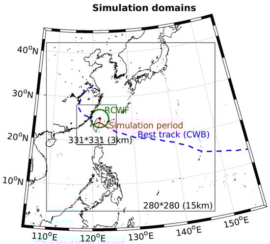
Figure 1.
The simulation domains of the two grids with two-way nesting, spanning and horizontal grid points at 15 km and 3 km resolutions, respectively. The green dot and circle are respectively the location and maximum unambiguous range of the Wufenshan (RCWF) radar. The blue dashed line is the best track of Typhoon Soudelor analyzed by CWB, where the red solid segment represents the simulation period (1200 UTC 7 August–0200 UTC 8 August) in this study.
The LETKF assimilation scheme is a variant of the square-root filter (also known as the deterministic EnKF), which does not require perturbing observations at analysis steps. Its distinguishing feature is that every grid point can be analyzed independently by assimilating surrounding observations within a covariance localization radius simultaneously. The complete algorithm can be found in Reference [64]. A noteworthy upgrade is made to the parallel computing framework of LETKF used in Reference [5] to improve assimilation efficiency for dense radar data. Suppose there are P processors available. In Reference [5], the grid to be analyzed was horizontally divided into P rectangular sub-grids of the same size, computed by separate processors. In this study, the grid to be analyzed is cut into y-z slices along the x direction, and the P processors take turns computing one slice at a time; that is, processor 1 computes slices 1, P + 1, 2P + 1, and so on. Both parallel computing frameworks give comparable efficiency if observations are evenly spread around the whole grid. However, if observations cluster in small areas as radar observations usually do, the latter framework gives higher efficiency for more balanced workload assigned to each processor. The configuration of LETKF in this study is largely inherited from Reference [5], which is optimized for the typhoon scenario. LETKF updates all prognostic state variables except , , , and . is excluded because of the difficulty in updating a two-dimensional vertically integrated field. , , and are left un-updated due to the concern about their highly non-Gaussian error statistics. Instead, these four variables are dynamically adjusted by the updated variables at the forecast steps of assimilation cycles. Applying the mixed localization method, which was first proposed in Reference [5], the horizontal covariance localization radii are 36 km for u and v and 12 km for the other updated variables to reflect the larger-scale error structure of horizontal winds in the typhoon scenario. The vertical covariance localization radius is uniformly 4 km. An ensemble size of 40 is used for limited computing resources, and a fixed multiplicative covariance inflation factor of 1.08 is used for the systematic underestimation of ensemble-based error covariances.
2.2. Observation Operator and Data Preprocessing
In Reference [5], the observation operator of WLRAS interpolated state variables from grid points to observation points and then converted them to and . Following Reference [72], the conversion to summed up the projections of u, v, w, and rainwater terminal velocity () on the radar beam, and the conversion to only considered the contribution from rainwater () with an assumed Marshall–Palmer DSD [73], as
where , , and are Cartesian coordinates with the origin at the radar site, and is the density of air. In this study, the observation operator of Reference [45] replaces the original operator (Equation (2)) to additionally consider the contribution from ice-phase hydrometeors, the bright band signature of the melting layer, and conversions to and . Firstly, a melting ice model is used to simulate the bright band signature resulting from mixed-phase hydrometeors that most bulk MP schemes do not deal with. Mixed-phase hydrometeors, such as rain-snow, rain-graupel, and rain-hail mixtures, are generated at a grid point by collecting a fraction of mass from rainwater and ice-phase hydrometeors if both coexist at that point, as
where denotes the ice-phase hydrometeor species, and is the maximum fraction, which empirically depends on the species. Secondly, backscattering amplitudes along horizontal and vertical axes are simulated as power-law functions of hydrometeor size that fit T-matrix scattering calculations [74] for rainwater and Rayleigh scattering calculations for ice-phase and mixed-phase hydrometeors. Reflectivity factors at horizontal and vertical polarizations ( and ) contributed from each hydrometeor species are then calculated by integrating backscattering cross-sections over a gamma DSD, and finally expressed as
where is the radar wavelength, is the dielectric constant of water, and are respectively the mixing ratio and density of the hydrometeor species, and are respectively the intercept and shape parameters of the gamma DSD, and are respectively the constant and exponent of the fitted power-law functions with subscripts and denoting horizontal and vertical axes, and , , and are coefficients that redeem the canting behavior of falling hydrometeors. Thirdly, contributed from each hydrometeor species is calculated by integrating the real part of the difference between forward scattering amplitudes along horizontal and vertical axes over the gamma DSD, and finally expressed as
where is also a coefficient that redeems the canting behavior. It is noteworthy that is prognostic in all SM, DM, and TM bulk MP schemes. is constant in SM schemes or diagnostic in DM and TM schemes as
where is prognostic in DM and TM schemes, and is constant in DM schemes or diagnostic in TM schemes with prognostic reflectivity. Hence, Equations (4)–(7) are solvable and applicable to all bulk MP schemes. Lastly, the contributions from all the hydrometeor species observable by weather radars to , , and are summed up to yield total values, in which total and yield and . Taking the WDM6 scheme, for example,
Besides the refined observation operator, appropriate data preprocessing and quality control to reduce observation errors also play an important role in real-case data assimilation. The polarimetric radar data used in this study come from the RCWF S-band polarimetric radar of CWB, located on the top of Mount Wufen (121.7725°E, 25.0728°N, 770 m altitude) on the northern coast of Taiwan (Figure 1). This radar is identical to the WSR-88D network in the U.S. with a maximum unambiguous range of 230 km, a volume scan interval of 7.5 min, and nine plan position indicator (PPI) elevation angles ranging from 0.5° to 19.5°. Quality control procedures, such as removing non-meteorological echoes, dealiasing data, and correcting signal attenuation, are fundamental to the preprocessing of raw radar data. Firstly, a high-resolution terrain file is used to filter out primary ground clutter, and then the remaining echoes are removed if < 0.8, an empirical value for the RCWF radar to distinguish between meteorological and non-meteorological echoes. Secondly, data are dealiased automatically with an algorithm that checks temporal and spatial continuity. Failed dealiasing is then manually unfolded. Thirdly, data are dealiased as well and then smoothed to estimate values, which are discarded if negative. Lastly, attenuation correction is applied to and data with a single-coefficient -based method [75], although the correction is almost negligible for the S band. Figure 2 shows the , , , and PPI observations, for the case of Typhoon Soudelor near landfall, at the lowest elevation angle posterior to the foregoing quality control procedures. It can be seen that most data-void areas and remaining noise are in the southwest quadrant where the higher Central Mountain Range is situated. The RCWF radar observations are thinned and interpolated to 19 constant altitude plan position indicator (CAPPI) altitudes ranging from 1 to 10 km at a 3 km horizontal resolution (corresponding to the fine grid) and 0.5 km vertical resolution prior to data assimilation. Observation errors are given as 1 m s−1 for , 2 dBZ for , 0.2 dB for , and 0.5° km−1 for referring to Reference [47].
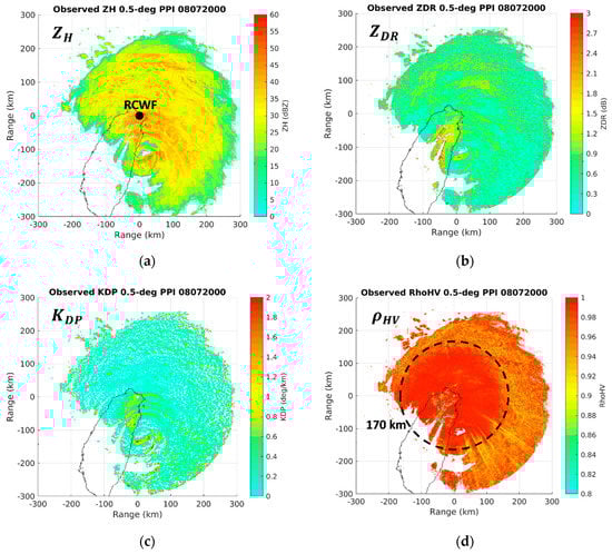
Figure 2.
The (a) reflectivity , (b) differential reflectivity , (c) specific differential phase , and (d) co-polar correlation coefficient PPI observations of the RCWF radar at a 0.5 degree elevation angle at 2000 UTC 7 August. The dot in panel (a) is the location of the RCWF radar. The dashed circle in panel (d) is a range of 170 km.
3. Case and Experiment Design
3.1. Case of Typhoon Soudelor
Typhoon Soudelor was the most devastating tropical cyclone in the Northwest Pacific region in 2015, resulting in dozens of fatalities and a tremendous loss of property on its way through the Northern Mariana Islands, Taiwan, and eastern China. Its westbound best track analyzed by CWB is shown in Figure 1, where the red solid segment represents the simulation period (1200 UTC 7 August–0200 UTC 8 August) in this study. This tropical cyclone reached tropical storm intensity on July 30, achieved Category 5 intensity with a minimum central pressure of 900 hPa and 10 min maximum sustained winds of 59.7 m s−1 on August 3, and struck the island of Taiwan with Category 3 intensity on August 7–8. During the hours around landfall on the eastern coast of Taiwan at 2040 UTC 7 August, strong gusts and rainbands north of the typhoon center severely impinged on northern Taiwan (Figure 2a) and damaged the RCWF radar by blowing its radome and antenna away. Nevertheless, Typhoon Soudelor was the first typhoon well observed by the RCWF radar after its polarimetric upgrade, and its valuable data obtained before the damage motivated this study.
At 2000 UTC 7 August, the eye of Typhoon Soudelor was located 110 km south of the RCWF radar (Figure 2a). The northern semicircle of Typhoon Soudelor, the so-called dangerous semicircle, consisted of several huge rainbands with reaching 50 dBZ. In contrast, fewer rainbands were evident and only close to the eye in the southern semicircle, and the most inner one featured a significant amount of large raindrops distinguished by high and values reaching 2.7 dB and 1.8° km−1, respectively (Figure 2b,c). and values inside the northern huge rainbands were lower over the ocean but increased over the land, especially . This indicates that orographic lifting affected rainbands moving toward terrain and resulted in stronger convection and precipitation. values were mostly higher than 0.98 within a range of 170 km but decrease beyond that (Figure 2d). This indicates that the melting layer was located at a 4 km altitude where mixed-phase hydrometeors existed. With respect to subsequent rainfall (Figure 3), three heavy rainfall areas (labeled A–C) were observed on the windward slopes of northern Taiwan with 3 h rainfall exceeding 150 mm during 2000–2300 UTC 7 August. Their locations correspond well to each rainband. During the next three hours, the rainfall decreased in northern Taiwan but increased in central Taiwan (area D) as the typhoon center gradually moved through central Taiwan. A 6 h maximum rainfall of 393 mm was reached in area A where massive disasters including floods, landslides, road closures, and the disruption of power and water supply occurred.
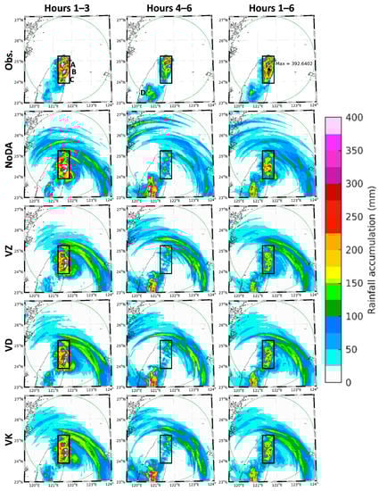
Figure 3.
The accumulated rainfall during (from left to right) 2000–2300 UTC 7 August, 2300 UTC 7 August–0200 UTC 8 August, and 2000 UTC 7 August–0200 UTC 8 August for (from top to bottom) the surface rain gauge observations and the forecasts of NoDA, VZ, VD, and VK (defined in Table 1). The green circle is the maximum unambiguous range of the RCWF radar. Uppercase A–D represent individual heavy rainfall areas, among which area A reaches a 6 h maximum rainfall of 393 mm. The black rectangle highlights areas A–C for easier visual comparison.
3.2. Experimental Design of Polarimetric Radar Data Assimilation
For the case of Typhoon Soudelor near landfall, a series of experiments are carried out to investigate the sensitivities of 6 h QPFs to polarimetric radar data assimilation. Figure 4 shows the schematic design of these experiments, aiming at improving a 6 h deterministic precipitation forecast for the most intense period since 2000 UTC 7 August. NoDA (no data assimilation) is a control experiment, which only performs a cold-start simulation initialized with the National Centers for Environmental Prediction (NCEP) Global Forecast System (GFS) 0.25 degree forecast at 1200 UTC 7 August. The initial eight and final six hours of the simulation are regarded as a model spin-up period and benchmark forecast, respectively. DA represents all the experiments that assimilate RCWF observations with the LETKF scheme, using a 40-member ensemble perturbed around the NoDA initial condition via the random-cv (random control variables) facility of the WRF 3DVar system. The initial ensemble goes through a 6 h spin-up period and nine assimilation cycles at a 15 min interval, and then the analysis ensemble mean is used to generate the 6 h deterministic forecast. Radar data assimilation only takes place in the fine grid, whose analysis increments are fed back to the coarse grid via two-way interaction. The predicted rainfalls on land in all the experiments are verified against the observed rainfall, interpolated from more than 750 surface rain gauges to the fine grid points. The locations of all the rain gauges are shown in Figure 5 as well as terrain contours and the verification area, the land within the 230 km maximum unambiguous range of the RCWF radar. The temporal resolution of rain gauge data is 10 min, and therefore, hourly accumulations can be calculated.
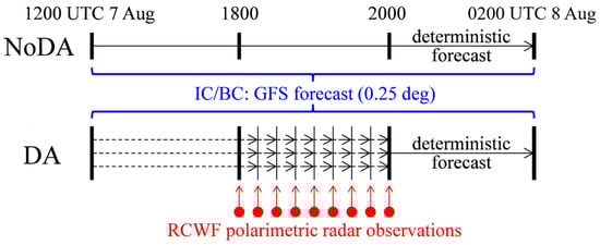
Figure 4.
The schematic design of the experiments on polarimetric radar data assimilation. NoDA is a control experiment, which performs a cold-start simulation initialized with the National Centers for Environmental Prediction (NCEP) Global Forecast System (GFS) 0.25 degree forecast at 1200 UTC 7 August. DA represents all the experiments that assimilate RCWF observations with the local ensemble transform Kalman filter (LETKF) scheme, using a 40-member ensemble perturbed around the NoDA initial condition.
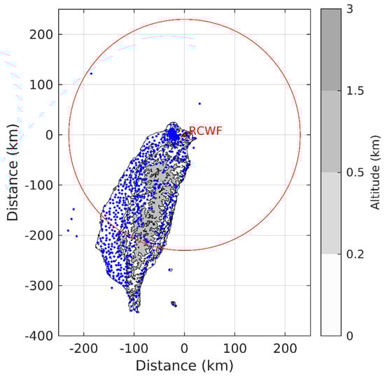
Figure 5.
The locations (blue dots) of more than 750 surface rain gauges in Taiwan. The terrain contours mark the altitudes of 0.2, 0.5, 1.5, and 3 km. The red dot and circle are respectively the location and maximum unambiguous range of the RCWF radar.
This study focuses on the sensitivities of QPFs to the assimilation of different radar variables, and therefore various combinations of radar variables are constructed for the DA experiments, as listed in Table 1. Uppercase V, Z, D, and K in the experiment names stand for assimilating , , , and , respectively. Because is linearly correlated to three-dimensional wind components and consequently beneficial for their analyses, as proved in Reference [5], it is assimilated in all the DA experiments. For , , and , only positive values are assimilated. Negative-value observations are rejected by the data assimilation system to avoid adverse impact because negative is around the limit of detection and negative and are against the assumption of oblate raindrops in the observation operator. The results of all the experiments are shown next in three parts: (1) the NoDA simulation and observation operator is assessed by examining the horizontal pattern and vertical distribution of simulated radar variables, (2) the analyzed radar variables and state variables in experiments VZ, VD, and VK are compared to distinguish the different impacts of assimilating , , and , and (3) the sensitivities of QPFs to different assimilated radar variables are revealed qualitatively and quantitatively.

Table 1.
The list of the experiments in this study.
4. Results
4.1. Assessment of NoDA Simulation and Observation Operator
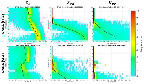
The NoDA simulation is first explored by comparing the forecast of , , and CAPPI fields with the RCWF radar observations at a 3.5 km altitude at 2000 UTC 7 August (Figure 6). A black rectangle is added to highlight the aforementioned areas A–C for easier visual comparison. Horizontally, NoDA exhibits significant differences of the rainband pattern and intensity from the observations. The simulated rainbands have position errors and look more discrete while the observed rainbands are connected with weaker echoes between. The intensity inside the simulated rainbands is generally overestimated for and . Despite these inconsistencies, the observed orographic lifting effect that strengthens convection and precipitation in areas A–C is still visible in the simulation. For overall vertical distribution, the contoured frequency by altitude diagrams (CFADs) with the median curve for , , and in convective precipitation areas (CPAs; defined by > 40 dBZ at a 3 km altitude) within the 230 km maximum unambiguous range at 2000 UTC 7 August are compared between the RCWF radar observations and NoDA (Figure 7). A blue rectangle is added to highlight the majority of the observed values at lower levels (below 5 km) for easier visual comparison, with ranges of 35–50 dBZ, 0.7–1.4 dB, and 0.2–0.7° km−1, respectively. The medians of the observed , , and all exhibit an increasing trend as the altitude decreases, which reflects the size-sorting mechanism that larger raindrops mostly exist at lower levels.
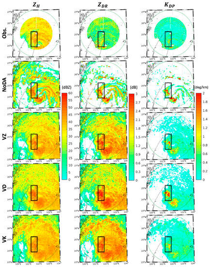
Figure 6.
The (from left to right) , , and constant altitude plan position indicator (CAPPI) fields at a 3.5 km altitude at 2000 UTC 7 August for the (from top to bottom) RCWF radar observations, NoDA forecast, VZ analysis ensemble mean, VD analysis ensemble mean, and VK analysis ensemble mean. The green circle is the maximum unambiguous range of the RCWF radar. The black rectangle highlights areas A–C for easier visual comparison.
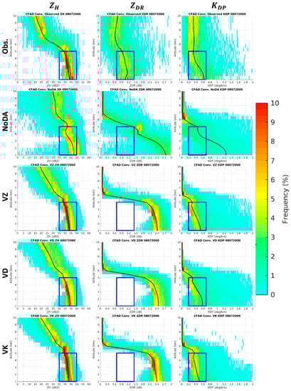
Figure 7.
The contoured frequency by altitude diagrams (CFADs) with the median curve for (from left to right) , , and in convective precipitation areas (CPAs) within the 230 km maximum unambiguous range at 2000 UTC 7 August for the (from top to bottom) RCWF radar observations, NoDA forecast, VZ analysis ensemble mean, VD analysis ensemble mean, and VK analysis ensemble mean. The blue rectangle highlights the majority of the observed values at lower levels for easier visual comparison.
The CFADs in stratiform precipitation areas (SPAs; defined by 10 dBZ < < 30 dBZ at a 3 km altitude) are also examined (Figure 8), although typhoon rainfall is dominated by the rainbands located in CPAs. The observed , , and values are similar to those in CPAs at higher levels but noticeably lower below, and the layer of the size-sorting mechanism is shallower (below 2.5 km). This result indicates that the absolute majority of raindrops in SPAs are smaller and more spherical. The NoDA simulation in SPAs has better consistency with the observations than in CPAs at lower levels, supporting Reference [76], that found the theoretical oblateness more accurate for smaller raindrops in typhoon cases. At higher levels in both CPAs and SPAs, the limitations of the observation operator for ice-phase hydrometeors are seen. It is noteworthy that the bright band signature, supposed to be clear near the melting layer of SPAs, is visible in the observations but excessive in the simulated and , especially an unrealistic spike between 4 and 6 km altitudes. This excess is proved attributable to the melting ice model of the observation operator because it vanishes if the model is ignored (Figure 9).
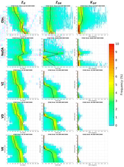
Figure 8.
As in Figure 7, but in stratiform precipitation areas (SPAs).
4.2. Comparison of the VZ, VD, and VK Analyses
To distinguish the different impacts of assimilating , , and , the final analyzed radar variables in experiments VZ, VD, and VK are compared with the foregoing NoDA simulation (Figure 6, Figure 7 and Figure 8). From the CAPPI fields at a 3.5 km altitude (Figure 6), all the three DA experiments correct the discrete rainband pattern in NoDA, but not all of them correct the overestimated intensity for and . Taking a closer look at the black rectangle highlighting areas A–C, the overestimation of is unchanged in VZ and VD but slightly mitigated in VK. In contrast, the overestimation of is better corrected in VZ and VK, the latter of which exhibits a very similar pattern to the observations. From the CFADs in CPAs (Figure 7), all three DA experiments rectify the excessive increasing trend for at lower levels rather than for , and VK shows the most realistic dispersion for the whole spectra of and in comparison to the observations. From the CFADs in SPAs (Figure 8), the three DA experiments resemble one another closely and correct the unrealistic bright band signature for and . These results about the analyzed radar variables can be generalized that, with the unadjusted observation operator, polarimetric radar data assimilation is still beneficial for analyses in this typhoon case. Besides, the different impacts of assimilating , , and are only distinguishable at the lower levels of CPAs where larger raindrops mostly exist, with a ranking order of , , and from best to worst. To further understand the variations of the analyzed state variables in the WRF model, Figure 10 shows the horizontal averages of w, , , , , , , and by altitude in CPAs within the 230 km maximum unambiguous range at 2000 UTC 7 August for experiments NoDA, V, VZ, VD, and VK. The results reveal that the NoDA simulation has particularly high values for w, , , , and , while the variations among the other DA experiments are more obvious for w, , , and . As is the state variable most related to rainfall, its ranking order of VK, VZ, V, VD, and NoDA from lowest to highest is to be compared with the skills of QPFs discussed next.
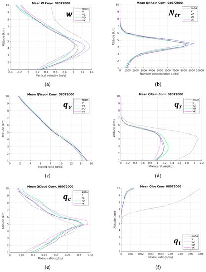
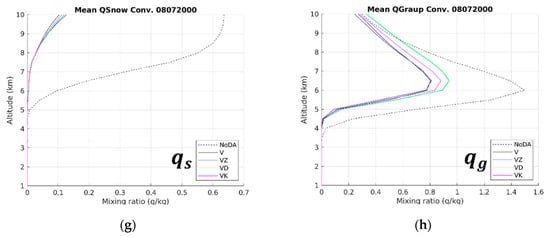
Figure 10.
The horizontal averages of (a) w, (b) , (c) , (d) , (e) , (f) , (g) , and (h) by altitude in CPAs within the 230 km maximum unambiguous range at 2000 UTC 7 August for experiments NoDA, V, VZ, VD, and VK.
4.3. Sensitivities of QPFs to Different Assimilated Radar Variables
The predicted rainfalls during the first three, second three, and total six hours of deterministic forecasts in experiments NoDA, VZ, VD, and VK are compared with the aforementioned observed rainfall (Figure 3). The black rectangle highlights areas A–C for easier visual comparison. During the first three hours, the patterns of areas A–C in the three DA experiments resemble the observations more than in NoDA. Outside the rectangle, the observed 3 h rainfall is generally lower than 50 mm (in blue), while NoDA and VD have more areas higher than 50 mm (in green and yellow) than VZ and VK. During the second three hours, all the NoDA and DA experiments have similar underestimates in areas A–C and overestimates in area D. This result implies that the positive effect of radar data assimilation on QPFs can last three hours in this study. As for the total 6 h accumulations, the improved pattern of areas A–C is diluted but still distinguishable in the three DA experiments. For quantitative verification, the root-mean-square error (RMSE), spatial correlation coefficient (SCC), and equitable threat score (ETS) on a threshold of 15 mm for the predicted hourly rainfall on land within the 230 km maximum unambiguous range during 2000 UTC 7 August–0200 UTC 8 August are compared in two groups of experiments (Figure 11). All the curves appear to be separate in the first three hours but tangled in the second three hours, and therefore reflect the 3 h positive impact of radar data assimilation again. Focusing on the first three hours, the ranking order from best (lowest RMSE, highest SCC, or highest ETS) to worst for the first group is VK, VZ, V, VD, and NoDA. This order is the same as the foregoing order from lowest to highest , which suggests that QPFs for this typhoon case highly depend on rainwater analyses. Moreover, the ranking order from best to worst for the second group is VZK, VZDK, VZD, VZ, and NoDA. This result suggests that, when and are already assimilated, further QPF improvement is still achievable by the additional assimilation of polarimetric variables, especially .
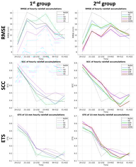
Figure 11.
The (from top to bottom) root-mean-square error (RMSE), spatial correlation coefficient (SCC), and equitable threat score (ETS) on a threshold of 15 mm for the predicted hourly rainfall on land within the 230 km maximum unambiguous range during 2000 UTC 7 August–0200 UTC 8 August in two groups of experiments.
5. Discussion
When examining the vertical distribution by CFADs in Figure 7, the increasing trend in NoDA is excessively simulated for and , especially , in accord with the overestimation shown in CAPPI. This serious overestimation inferentially originates from an unsuitable raindrop shape-size relation applied by the observation operator rather than a model wet bias for the two following reasons. One is that the overestimation is maximal for and minimal for respectively, having the most direct and indirect relations to the raindrop shape among the three variables. The other is that, according to Reference [76], examining in-situ 2D video disdrometer observations for 13 typhoons that struck Taiwan, the raindrops larger than 1.5 mm under high horizontal winds tend to be more spherical than the theoretical ones in References [37] and [77], referred to by Reference [45] and in this study.
At higher levels (above 5 km), the observed , , and values generally become lower, except for a few outliers. This result corresponds with the observations in Reference [78] for the case of Typhoon Nida (2016), asserting that lower values are mainly contributed from widespread snow, while a few higher values are contributed from supercooled rainwater and mixed-phase hydrometeors in updraft regions. However, the simulated and are seriously underestimated with overwhelming near-zero values. This serious underestimation inferentially originates from the limitations of the observation operator for ice-phase hydrometeors in the three following aspects. Firstly, snow, graupel, and hail are all treated as ice ellipsoids with the same axis ratio during Rayleigh scattering calculations, while the true shapes are all different. Secondly, Mie scattering calculations may be more realistic for giant ice-phase hydrometeors like hailstones. Lastly, ice crystals, which are not considered in the observation operator, could be observable by weather radars when they are vertically aligned or canted by electric fields [79].
Hence, the NoDA simulation exposes three sources of the observation operator errors, including the raindrop shape-size relation, the limitations for ice-phase hydrometeors, and the melting ice model. These error sources all deserve further studies of optimization for typhoon cases.
6. Summary and Future Prospects
Typhoon Soudelor has been the most completely observed typhoon by the RCWF S-band polarimetric radar in Taiwan up to the present. No other typhoons have impinged on northern Taiwan as severely as Typhoon Soudelor did, and therefore, the polarimetric radar observations near the landfall of Typhoon Soudelor are precious and unique. This study uses the WDM6 microphysical scheme and incorporates the observation operator of Reference [45] into the WRF-LETKF radar assimilation system to investigate the sensitivities of 6 h QPFs for Typhoon Soudelor near landfall to the assimilation of the RCWF radar observations. The configuration of the WRF model refers to an operational run from Taiwan’s Central Weather Bureau, and the configuration of LETKF is largely inherited from Reference [5]. After the quality control, thinning, and interpolation of the radar observations, a series of experiments assimilating various combinations of radar variables are carried out and compared with a control simulation without radar data assimilation for the purpose of improving a 6 h deterministic precipitation forecast for the most intense period since 2000 UTC 7 August. The results of the control simulation expose three sources of the observation operator errors, including the raindrop shape-size relation, the limitations for ice-phase hydrometeors, and the melting ice model. Nevertheless, this study inherits the default observation operator of Reference [45] and concludes that polarimetric radar data assimilation with the unadjusted observation operator can still improve the analyses of state variables, especially rainwater, and consequent QPFs for this typhoon case. The different impacts of assimilating , , and are only distinguishable at the lower levels of convective precipitation areas, with a ranking order of , , and from best to worst. Finally, the positive effect of radar data assimilation on QPFs can last three hours in this study, and further QPF improvement is achievable by the additional assimilation of polarimetric variables, especially , on top of and .
For future prospects, further studies as stated above can be focused on suppressing the three sources of the observation operator errors exposed by the control simulation. The theoretical raindrop shape-size relation can be easily replaced with the in-situ one for typhoons in Reference [76] to re-simulate the scattering amplitudes via the T-matrix scattering calculations for rainwater. In contrast, the limitations for ice-phase hydrometeors are too difficult to deal with, and therefore ignoring the assimilation of polarimetric variables at higher levels can be a good strategy to adopt. As for the melting ice model, adjustment can be more meaningful than disuse because it is theoretically tenable to consider mixed-phase hydrometeors for the bright band signature. For example, a study joined by the authors recently found that, for an MCS case in Taiwan, the excessively simulated bright band signature can be mitigated when a minimum threshold of number concentrations for mixed-phase hydrometeors is applied to the melting ice model [80]. With a more accurate observation operator, the contribution from polarimetric variables can be more robust and also expectable for different types of precipitation systems. The results will be more representative of general performance if more cases are available and evaluated.
Author Contributions
Conceptualization, C.-C.T. and K.-S.C.; methodology, C.-C.T. and K.-S.C.; software, C.-C.T.; validation, C.-C.T.; formal analysis, C.-C.T.; writing—original draft preparation, C.-C.T.; supervision, K.-S.C.; funding acquisition, C.-C.T. All authors have read and agreed to the published version of the manuscript.
Funding
This research was funded by Taiwan’s National Science and Technology Center for Disaster Reduction (NCDR) as well as Ministry of Science and Technology (MOST) under Grants MOST-104-2111-M-492-001, MOST-105-2111-M-492-004, and MOST-106-2119-M-492-005.
Acknowledgments
The authors are grateful to Prof. Youngsun Jung from the Center for Analysis and Prediction of Storms, University of Oklahoma, for her invaluable guidance on the observation operator and suggestions about this study. All the comments from the peer reviewers and discussions with Prof. Shu-Chih Yang from the National Central University in Taiwan are also appreciated.
Conflicts of Interest
The authors declare no conflict of interest.
References
- Wu, C.-C.; Chou, K.-H.; Lin, P.-H.; Aberson, S.D.; Peng, M.S.; Nakazawa, T. The impact of dropwindsonde data on typhoon track forecasts in DOTSTAR. Weather Forecast. 2007, 22, 1157–1176. [Google Scholar] [CrossRef]
- Huang, C.-Y.; Huang, C.-H.; Skamarock, W.C. Track deflection of Typhoon Nesat (2017) as realized by multi-resolution simulations of a global model. Mon. Weather Rev. 2019, 147, 1593–1613. [Google Scholar] [CrossRef]
- Hong, J.-S.; Fong, C.-T.; Hsiao, L.-F.; Yu, Y.-C.; Tzeng, C.-Y. Ensemble typhoon quantitative precipitation forecasts model in Taiwan. Weather Forecast. 2015, 30, 217–237. [Google Scholar] [CrossRef]
- Wang, C.-C.; Huang, S.-Y.; Chen, S.-H.; Chang, C.-S.; Tsuboki, K. Cloud-resolving typhoon rainfall ensemble forecasts for Taiwan with large domain and extended range through time-lagged approach. Weather Forecast. 2016, 31, 151–172. [Google Scholar] [CrossRef]
- Tsai, C.-C.; Yang, S.-C.; Liou, Y.-C. Improving quantitative precipitation nowcasting with a local ensemble transform Kalman filter radar data assimilation system: Observing system simulation experiments. Tellus A 2014, 66, 21804. [Google Scholar] [CrossRef]
- Wang, M.; Xue, M.; Zhao, K.; Dong, J. Assimilation of T-TREC-retrieved winds from single-Doppler radar with an ensemble Kalman filter for the forecast of Typhoon Jangmi (2008). Mon. Weather Rev. 2014, 142, 1892–1907. [Google Scholar] [CrossRef]
- Mandapaka, P.V.; Germann, U.; Panziera, L.; Hering, A. Can Lagrangian extrapolation of radar fields be used for precipitation nowcasting over complex Alpine orography? Weather Forecast. 2012, 27, 28–49. [Google Scholar] [CrossRef]
- Otsuka, S.; Tuerhong, G.; Kikuchi, R.; Kitano, Y.; Taniguchi, Y.; Ruiz, J.J.; Satoh, S.; Ushio, T.; Miyoshi, T. Precipitation nowcasting with three-dimensional space-time extrapolation of dense and frequent phased-array weather radar observations. Weather Forecast. 2016, 31, 329–340. [Google Scholar] [CrossRef]
- Sun, J.; Xue, M.; Wilson, J.W.; Zawadzki, I.; Ballard, S.P.; Onvlee-Hooimeyer, J.; Joe, P.; Barker, D.; Li, P.-W.; Golding, B.; et al. Use of NWP for nowcasting convective precipitation: Recent progress and challenges. Bull. Am. Meteorol. Soc. 2014, 95, 409–426. [Google Scholar] [CrossRef]
- Hwang, Y.; Clark, A.J.; Lakshmanan, V.; Koch, S.E. Improved nowcasts by blending extrapolation and model forecasts. Weather Forecast. 2015, 30, 1201–1217. [Google Scholar] [CrossRef]
- Chung, K.-S.; Yao, I.-A. Improving radar echo Lagrangian extrapolation nowcasting by blending numerical model wind information: Statistical performance of 16 typhoon cases. Mon. Weather Rev. 2020, 148, 1099–1120. [Google Scholar] [CrossRef]
- Xiao, Q.; Sun, J. Multiple-radar data assimilation and short-range quantitative precipitation forecasting of a squall line observed during IHOP_2002. Mon. Weather Rev. 2007, 135, 3381–3404. [Google Scholar] [CrossRef]
- Sugimoto, S.; Crook, N.A.; Sun, J.; Xiao, Q.; Barker, D.M. An examination of WRF 3DVAR radar data assimilation on its capability in retrieving unobserved variables and forecasting precipitation through Observing System Simulation Experiments. Mon. Weather Rev. 2009, 137, 4011–4029. [Google Scholar] [CrossRef]
- Hong, S.-Y.; Lim, J.-O.J. The WRF single-moment 6-class microphysics scheme (WSM6). J. Korean Meteorol. Soc. 2006, 42, 129–151. [Google Scholar]
- Sasaki, Y. An objective analysis based on the variational method. J. Meteorol. Soc. Jpn. 1958, 36, 77–88. [Google Scholar] [CrossRef]
- Bao, X.; Wu, D.; Lei, X.; Ma, L.; Wang, D.; Zhao, K.; Jou, B.J.-D. Improving the extreme rainfall forecast of Typhoon Morakot (2009) by assimilating radar data from Taiwan Island and mainland China. J. Meteorol. Res. 2017, 31, 747–766. [Google Scholar] [CrossRef]
- Jung, Y.; Xue, M.; Zhang, G.F. Simulations of polarimetric radar signatures of a supercell storm using a two-moment bulk microphysics scheme. J. Appl. Meteorol. Climatol. 2010, 49, 146–163. [Google Scholar] [CrossRef]
- Jung, Y.; Xue, M.; Tong, M. Ensemble Kalman filter analyses of the 29-30 May 2004 Oklahoma tornadic thunderstorm using one- and two-moment bulk microphysics schemes, with verification against polarimetric radar data. Mon. Weather Rev. 2012, 140, 1457–1475. [Google Scholar] [CrossRef]
- Dawson, D.T., II; Xue, M.; Milbrandt, J.A.; Yau, M.K. Comparison of evaporation and cold pool development between single-moment and multimoment bulk microphysics schemes in idealized simulations of tornadic thunderstorms. Mon. Weather Rev. 2010, 138, 1152–1171. [Google Scholar] [CrossRef]
- Dawson, D.T., II; Mansell, E.R.; Jung, Y.; Wicker, L.J.; Kumjian, M.R.; Xue, M. Low-level ZDR signatures in supercell forward flanks: The role of size sorting and melting of hail. J. Atmos. Sci. 2014, 71, 276–299. [Google Scholar] [CrossRef]
- Johnson, M.; Jung, Y.; Dawson, D.T., II; Xue, M. Comparison of simulated polarimetric signatures in idealized supercell storms using two-moment bulk microphysics schemes in WRF. Mon. Weather Rev. 2016, 144, 971–996. [Google Scholar] [CrossRef]
- Putnam, B.J.; Xue, M.; Jung, Y.; Zhang, G.; Kong, F. Simulation of polarimetric radar variables from 2013 CAPS spring experiment storm-scale ensemble forecasts and evaluation of microphysics schemes. Mon. Weather Rev. 2017, 145, 49–73. [Google Scholar] [CrossRef]
- Labriola, J.; Snook, N.; Jung, Y.; Putnam, B.; Xue, M. Ensemble hail prediction for the storms of 10 May 2010 in south-central Oklahoma using single- and double-moment microphysical schemes. Mon. Weather Rev. 2017, 145, 4911–4936. [Google Scholar] [CrossRef]
- Putnam, B.J.; Xue, M.; Jung, Y.; Snook, N.; Zhang, G. The analysis and prediction of microphysical states and polarimetric radar variables in a mesoscale convective system using double-moment microphysics, multinetwork radar data, and the ensemble Kalman filter. Mon. Weather Rev. 2014, 142, 141–162. [Google Scholar] [CrossRef]
- Putnam, B.J.; Xue, M.; Jung, Y.; Snook, N.A.; Zhang, G. Ensemble probabilistic prediction of a mesoscale convective system and associated polarimetric radar variables using single-moment and double-moment microphysics schemes and EnKF radar data assimilation. Mon. Weather Rev. 2017, 145, 2257–2279. [Google Scholar] [CrossRef]
- Brown, B.R.; Bell, M.M.; Frambach, A.J. Validation of simulated hurricane drop size distributions using polarimetric radar. Geophys. Res. Lett. 2016, 43, 910–917. [Google Scholar] [CrossRef]
- Le Dimet, F.-X.; Talagrand, O. Variational algorithms for analysis and assimilation of meteorological observations: Theoretical aspects. Tellus 1986, 38A, 97–110. [Google Scholar] [CrossRef]
- Evensen, G. Sequential data assimilation with a nonlinear quasi-geostrophic model using Monte Carlo methods to forecast error statistics. J. Geophys. Res. 1994, 99, 10143–10162. [Google Scholar] [CrossRef]
- Hamill, T.M.; Snyder, C. A hybrid ensemble Kalman filter-3D variational analysis scheme. Mon. Weather Rev. 2000, 128, 2905–2919. [Google Scholar] [CrossRef]
- Del Moral, P. Nonlinear filtering using random particles. Theory Probab. Appl. 1996, 40, 690–701. [Google Scholar] [CrossRef]
- Zhang, F.; Weng, Y.; Sippel, J.A.; Meng, Z.; Bishop, C.H. Cloud-resolving hurricane initialization and prediction through assimilation of Doppler radar observations with an ensemble Kalman filter. Mon. Weather Rev. 2009, 137, 2105–2125. [Google Scholar] [CrossRef]
- Li, Y.; Wang, X.; Xue, M. Assimilation of radar radial velocity data with the WRF hybrid ensemble-3DVAR system for the prediction of Hurricane Ike (2008). Mon. Weather Rev. 2012, 140, 3507–3524. [Google Scholar] [CrossRef]
- Sun, J.; Wang, H. Radar data assimilation with WRF 4D-Var. Part II: Comparison with 3D-Var for a squall line over the U.S. Great Plains. Mon. Weather Rev. 2013, 141, 2245–2264. [Google Scholar] [CrossRef]
- Johnson, A.; Wang, X.; Carley, J.R.; Wicker, L.J.; Karstens, C. A comparison of multiscale GSI-based EnKF and 3DVar data assimilation using radar and conventional observations for midlatitude convective-scale precipitation forecasts. Mon. Weather Rev. 2015, 143, 3087–3108. [Google Scholar] [CrossRef]
- Kong, R.; Xue, M.; Liu, C. Development of a hybrid En3DVar data assimilation system and comparisons with 3DVar and EnKF for radar data assimilation with observing system simulation experiments. Mon. Weather Rev. 2018, 146, 175–198. [Google Scholar] [CrossRef]
- Putnam, B.; Xue, M.; Jung, Y.; Snook, N.; Zhang, G. Ensemble Kalman filter assimilation of polarimetric radar observations for the 20 May 2013 Oklahoma tornadic supercell case. Mon. Weather Rev. 2019, 147, 2511–2533. [Google Scholar] [CrossRef]
- Green, A.W. An approximation for the shapes of large raindrops. J. Appl. Meteorol. Climatol. 1975, 14, 1578–1583. [Google Scholar] [CrossRef]
- Zrnic, D.S.; Ryzhkov, A.V. Polarimetry for weather surveillance radars. Bull. Am. Meteorol. Soc. 1999, 80, 389–406. [Google Scholar] [CrossRef]
- Cunha, L.K.; Smith, J.A.; Baeck, M.L.; Krajewski, W.F. An early performance evaluation of the NEXRAD dual-polarization radar rainfall estimates for urban flood applications. Weather Forecast. 2013, 28, 1478–1497. [Google Scholar] [CrossRef]
- Huuskonen, A.; Saltikoff, E.; Holleman, I. The operational weather radar network in Europe. Bull. Am. Meteorol. Soc. 2014, 95, 897–907. [Google Scholar] [CrossRef]
- Brandes, E.A.; Zhang, G.; Vivekanandan, J. Experiments in rainfall estimation with a polarimetric radar in a subtropical environment. J. Appl. Meteorol. 2002, 41, 674–685. [Google Scholar] [CrossRef]
- Giangrande, S.E.; Ryzhkov, A.V. Estimation of rainfall based on the results of polarimetric echo classification. J. Appl. Meteorol. Climatol. 2008, 47, 2445–2462. [Google Scholar] [CrossRef]
- Matrosov, S.Y. Evaluating polarimetric X-band radar rainfall estimators during HMT. J. Atmos. Oceanic Technol. 2010, 27, 122–134. [Google Scholar] [CrossRef]
- Wang, Y.; Chandrasekar, V. Quantitative precipitation estimation in the CASA X-band dual-polarization radar network. J. Atmos. Oceanic Technol. 2010, 27, 1665–1676. [Google Scholar] [CrossRef]
- Jung, Y.; Zhang, G.; Xue, M. Assimilation of simulated polarimetric radar data for a convective storm using the ensemble Kalman filter. Part I: Observation operators for reflectivity and polarimetric variables. Mon. Weather Rev. 2008, 136, 2228–2245. [Google Scholar] [CrossRef]
- Pfeifer, M.; Craig, G.C.; Hagen, M.; Keil, C. A polarimetric radar forward operator for model evaluation. J. Appl. Meteorol. Climatol. 2008, 47, 3202–3220. [Google Scholar] [CrossRef]
- Jung, Y.; Xue, M.; Zhang, G.; Straka, J.M. Assimilation of simulated polarimetric radar data for a convective storm using the ensemble Kalman filter. Part II: Impact of polarimetric data on storm analysis. Mon. Weather Rev. 2008, 136, 2246–2260. [Google Scholar] [CrossRef]
- Jung, Y.; Xue, M.; Zhang, G. Simultaneous estimation of microphysical parameters and the atmospheric state using simulated polarimetric radar data and an ensemble Kalman filter in the presence of an observation operator error. Mon. Weather Rev. 2010, 138, 539–562. [Google Scholar] [CrossRef]
- Lin, Y.-L.; Farley, R.D.; Orville, H.D. Bulk parameterization of the snow field in a cloud model. J. Climate Appl. Meteorol. 1983, 22, 1065–1092. [Google Scholar] [CrossRef]
- Li, X.; Mecikalski, J.R. Assimilation of the dual-polarization Doppler radar data for a convective storm with a warm-rain radar forward operator. J. Geophys. Res. 2010, 115, D16208. [Google Scholar] [CrossRef]
- Kessler, E. On the distribution and continuity of water substance in atmospheric circulation. Meteorol. Monogr. 1969, 32, 84. [Google Scholar] [CrossRef]
- Li, X.; Mecikalski, J.R.; Posselt, D. An ice-phase microphysics forward model and preliminary results of polarimetric radar data assimilation. Mon. Weather Rev. 2017, 145, 683–708. [Google Scholar] [CrossRef]
- Carlin, J.T.; Gao, J.; Snyder, J.C.; Ryzhkov, A.V. Assimilation of ZDR columns for improving the spinup and forecast of convective storms in storm-scale models: Proof-of-concept experiments. Mon. Weather Rev. 2017, 145, 5033–5057. [Google Scholar] [CrossRef]
- Hu, M.; Xue, M.; Brewster, K. 3DVAR and cloud analysis with WSR-88D level-II data for the prediction of the Fort Worth, Texas, tornadic thunderstorms. Part I: Cloud analysis and its impact. Mon. Weather Rev. 2006, 134, 675–698. [Google Scholar] [CrossRef]
- Milbrandt, J.A.; Yau, M.K. A multimoment bulk microphysics parameterization. Part I: Analysis of the role of the spectral shape parameter. J. Atmos. Sci. 2005, 62, 3051–3064. [Google Scholar] [CrossRef]
- Augros, C.; Caumont, O.; Ducrocq, V.; Gaussiat, N. Assimilation of radar dual-polarization observations in the AROME model. Q. J. R. Meteorol. Soc. 2018, 144, 1352–1368. [Google Scholar] [CrossRef]
- Seity, Y.; Brousseau, P.; Malardel, S.; Hello, G.; Bénard, P.; Bouttier, F.; Lac, C.; Masson, V. The AROME-France convective-scale operational model. Mon. Weather Rev. 2011, 139, 976–991. [Google Scholar] [CrossRef]
- Pinty, J.P.; Jabouille, P. A mixed-phased cloud parameterization for use in a mesoscale non-hydrostatic model: Simulations of a squall line and of orographic precipitation. In Proceedings of the Conference on Cloud Physics, Everett, WA, USA, 17–21 August 1998; Preprints. pp. 217–220. [Google Scholar]
- Kawabata, T.; Bauer, H.-S.; Schwitalla, T.; Wulfmeyer, V.; Adachi, A. Evaluation of forward operators for polarimetric radars aiming for data assimilation. J. Meteorol. Soc. Jpn. 2018, 96A, 157–174. [Google Scholar] [CrossRef]
- Kawabata, T.; Schwitalla, T.; Adachi, A.; Bauer, H.-S.; Wulfmeyer, V.; Nagumo, N.; Yamauchi, H. Observational operators for dual polarimetric radars in variational data assimilation systems (PolRad VAR v1.0). Geosci. Model Dev. 2018, 11, 2493–2501. [Google Scholar] [CrossRef]
- Skamarock, W.C.; Klemp, J.B.; Dudhia, J.; Gill, D.O.; Liu, Z.; Berner, J.; Wang, W.; Powers, J.G.; Duda, M.G.; Barker, D.M.; et al. A description of the Advanced Research WRF Model Version 4; National Center for Atmospheric Research: Boulder, CO, USA, 2019; p. 145. [Google Scholar] [CrossRef]
- Saito, K. The JMA nonhydrostatic model and its applications to operation and research. In Atmospheric Model Applications; Yucel, I., Ed.; IntechOpen: London, UK, 2012; pp. 85–110. [Google Scholar] [CrossRef]
- Whitaker, J.S.; Hamill, T.M. Ensemble data assimilation without perturbed observations. Mon. Weather Rev. 2002, 130, 1913–1924. [Google Scholar] [CrossRef]
- Hunt, B.R.; Kostelich, E.J.; Szunyogh, I. Efficient data assimilation for spatiotemporal chaos: A local ensemble transform Kalman filter. Physica D 2007, 230, 112–126. [Google Scholar] [CrossRef]
- Lim, K.-S.S.; Hong, S.-Y. Development of an effective double-moment cloud microphysics scheme with prognostic cloud condensation nuclei (CCN) for weather and climate models. Mon. Weather Rev. 2010, 138, 1587–1612. [Google Scholar] [CrossRef]
- Mlawer, E.J.; Taubman, S.J.; Brown, P.D.; Iacono, M.J.; Clough, S.A. Radiative transfer for inhomogeneous atmosphere: RRTM, a validated correlated-k model for the longwave. J. Geophys. Res. 1997, 102, 16663–16682. [Google Scholar] [CrossRef]
- Chou, M.-D.; Suarez, M.J. An Efficient Thermal Infrared Radiation Parameterization for Use in General Circulation Models; National Aeronautics and Space Administration: Washington, DC, USA, 1994; Volume 104606, pp. 1–85.
- Jiménez, P.A.; Dudhia, J.; González-Rouco, J.F.; Navarro, J.; Montávez, J.P.; García-Bustamante, E. A revised scheme for the WRF surface layer formulation. Mon. Weather Rev. 2012, 140, 898–918. [Google Scholar] [CrossRef]
- Chen, F.; Dudhia, J. Coupling an advanced land surface-hydrology model with the Penn State-NCAR MM5 modeling system. Part I: Model implementation and sensitivity. Mon. Weather Rev. 2001, 129, 569–585. [Google Scholar] [CrossRef]
- Hong, S.-Y.; Noh, Y.; Dudhia, J. A new vertical diffusion package with an explicit treatment of entrainment processes. Mon. Weather Rev. 2006, 134, 2318–2341. [Google Scholar] [CrossRef]
- Kain, J.S. The Kain-Fritsch convective parameterization: An update. J. Appl. Meteorol. 2004, 43, 170–181. [Google Scholar] [CrossRef]
- Sun, J.; Crook, N.A. Dynamical and microphysical retrieval from Doppler radar observations using a cloud model and its adjoint. Part I: Model development and simulated data experiments. J. Atmos. Sci. 1997, 54, 1642–1661. [Google Scholar] [CrossRef]
- Marshall, J.S.; Palmer, W.M.K. The distribution of raindrops with size. J. Meteorol. 1948, 5, 165–166. [Google Scholar] [CrossRef]
- Waterman, P.C. Scattering by dielectric obstacles. Alta Freq. 1969, 38, 348–352. [Google Scholar]
- Bringi, V.N.; Chandrasekar, V.; Balakrishnan, N.; Zrnic, D. An examination of propagation effects in rainfall on radar measurements at microwave frequencies. J. Atmos. Ocean. Technol. 1990, 7, 829–840. [Google Scholar] [CrossRef]
- Chang, W.-Y.; Wang, T.-C.C.; Lin, P.-L. Characteristics of the raindrop size distribution and drop shape relation in typhoon systems in the western Pacific from the 2D video disdrometer and NCU C-Band polarimetric radar. J. Atmos. Ocean. Technol. 2009, 26, 1973–1993. [Google Scholar] [CrossRef]
- Zhang, G.; Vivekanandan, J.; Brandes, E. A method for estimating rain rate and drop size distribution from polarimetric radar measurements. IEEE Trans. Geosci. Remote Sens. 2001, 39, 830–841. [Google Scholar] [CrossRef]
- Wu, D.; Zhao, K.; Kumjian, M.R.; Chen, X.; Huang, H.; Wang, M.; Didlake, A.C., Jr.; Duan, Y.; Zhang, F. Kinematics and microphysics of convection in the outer rainband of Typhoon Nida (2016) revealed by polarimetric radar. Mon. Weather Rev. 2018, 146, 2147–2159. [Google Scholar] [CrossRef]
- Hubbert, J.C.; Ellis, S.M.; Chang, W.-Y.; Rutledge, S.; Dixon, M. Modeling and interpretation of S-band ice crystal depolarization signatures from data obtained by simultaneously transmitting horizontally and vertically polarized fields. J. Appl. Meteorol. Climatol. 2014, 53, 1659–1677. [Google Scholar] [CrossRef]
- You, C.-R.; Chung, K.-S.; Tsai, C.-C. Evaluating the performance of a convection-permitting model by using dual-polarimetric radar parameters: Case study of SoWMEX-IOP8. Remote Sens. 2020, 12, 3004. [Google Scholar] [CrossRef]
Publisher’s Note: MDPI stays neutral with regard to jurisdictional claims in published maps and institutional affiliations. |
© 2020 by the authors. Licensee MDPI, Basel, Switzerland. This article is an open access article distributed under the terms and conditions of the Creative Commons Attribution (CC BY) license (http://creativecommons.org/licenses/by/4.0/).