Abstract
Coastal dunes have global importance as ecological habitats, recreational areas, and vital natural coastal protection. Dunes evolve due to variations in the supply and removal of sediment via both wind and waves, and on stabilization through vegetation colonization and growth. One aspect of dune evolution that is poorly understood is the longshore variation in dune response to morphodynamic forcing, which can occur over small spatial scales. In this paper, a fixed wing unmanned aerial vehicle (UAV), is used to measure the longshore variation in evolution of a dune system in a megatidal environment. Dune sections to the east and west of the study site are prograding whereas the central portion is static or eroding. The measured variation in dune response is compared to mesoscale intertidal bar migration and short-term measurements of longshore variation in wave characteristics during two storms. Intertidal sand bar migration is measured using satellite imagery: crescentic intertidal bars are present in front of the accreting portion of the beach to the west and migrate onshore at a rate of 0.1–0.2 m/day; episodically the eastern end of the bar detaches from the main bar and migrates eastward to attach near the eastern end of the study area; bypassing the central eroding section. Statistically significant longshore variation in intertidal wave heights were measured using beachface mounted pressure transducers: the largest significant wave heights are found in front of the dune section suffering erosion. Spectral differences were noted with more narrow-banded spectra in this area but differences are not statistically significant. These observations demonstrate the importance of three-dimensionality in intertidal beach morphology on longshore variation in dune evolution; both through longshore variation in onshore sediment supply and through causing longshore variation in near-dune significant wave heights.
1. Introduction
In this paper, we investigate the evolution of a coastal dune system in a megatidal environment (spring tidal range >8 m) at Crymlyn Burrows, Swansea Bay, UK. Specifically, we seek to understand the factors that cause longshore variation in dune morphotype and evolution that were measured by unmanned aerial vehicle (UAV).
Coastal dunes are of vital importance as coastal defences, unique ecological habitats and recreational areas [1]. For example, their coastal protection function has been valued in the US as $86,000 per hectare per year [2]. In recent years, observations have been made of increased vegetation and stabilization of coastal dunes [3,4], leading to vigorous debate on the appropriateness of intervention [5,6] and research into intervention efficacy, e.g., [7,8]. Proper understanding of the drivers of dune evolution in all forms of coastal environment is required to inform an adequate suite of management practices.
The evolution of coastal dunes is a complex interaction between beach morphology, aeolian sediment transport, wave-driven sediment transport and biological factors. Aeolian transport supplies sand to the dune area not only under cross-shore and onshore flow [9,10] but also under offshore directed winds due to recirculation over the dune crest [11]. Intertidal beach shape affects aeolian transport to the dune, with dissipative beaches most favourable for aeolian supply [12]. Equally, dependent on dune morphology, offshore winds can move sediment from the dune to the backshore and intertidal [13,14], renourishing the intertidal beach. Dune vegetation helps to trap dune directed aeolian sediment supply [15,16] and also stabilizes the dune from erosion by wind [17] and waves [18]. Waves are typically considered from an erosive perspective in relation to dune systems e.g., [19,20,21,22,23,24,25]; however, there is a recognition that wave-driven onshore transport can provide sediment reservoirs that subsequently can nourish dunes through aeolian transport [26,27,28]. Spatial variation in foredune evolution has been noted over a range of scales [29,30,31,32]. Understanding the driving factors for this variation is important to facilitate appropriate management. Over regional scales in Northern France, Héquette, et al. [32] find that surge elevation is more important than wave height in describing spatial variation in dune erosion and also note the importance of upper intertidal beach width. Over the 3.6 km Narrabeen embayment (Australia), Splinter, et al. [29] find dune erosion is best related to pre-storm dune toe elevation. Over smaller scales, Brodie, et al. [30] assessed two 50 m sections of dune separated by 700 m that underwent similar aeolian and hydrodynamic forcing; one section accreted and the other eroded which was linked to variation in starting morphology. Brodie, et al. [30] also note that insufficient research has been conducted on spatial variation in dune response to adequately understand the relevant processes; something this paper deals with.
Megatidal environments, where the mean spring tidal range is greater than 8 m [33], form the end-member of the tidal range continuum. Sandy beaches in these environments are typically ultra-dissipative (shallow beach gradient) in the lower intertidal with increasing gradient in the upper intertidal [33]. Varying beach gradient and large tidal ranges mean that wave dissipation through bottom friction can be tidally modulated leading to tidal modulation of wave heights which are larger at high tide [34]. Tidal currents can be strong and lower intertidal zones tide dominated in contrast to wave dominated mid-tidal zones for these environments [34]. An indirect effect of large tidal ranges is the rapid translation of different breaker zones over the shoreface [35] which tends to subdue morphological change [33]. Minimal research has been conducted on the behaviour of coastal dunes in megatidal settings; Karunarathna, et al. [36] investigated the beach-dune system at Sefton, UK; but focus was on the beach rather than the dune. As tidal range increases, the sequencing of storm and surge events become more important in the evolution of coastal dunes. Wave and surge events have to occur at high tide to impact the dune system and equally aeolian transport is increasingly tidally modulated. Therefore, it is likely that dune evolution may be different to that at sites with lower tidal range and hence there is a requirement to study their behavior.
Dune evolution may be effectively monitored through UAVs, commonly called drones. This technology has found a wide range of uses in coastal research: primarily photogrammetry with RGB cameras to map morphology [37,38,39,40,41]; RGB data has also been used for vegetation studies [42]; LiDAR based morphology has been recorded from UAVs [43]; and, multispectral cameras have been used for vegetation studies [44,45,46] and for sediment classification [47]. Both fixed wing, e.g., [40], and quadcopter drones, e.g., [48] have been used. Drones with real-time kinematic (RTK) GPS have been used to improve the accuracy of returned solutions, e.g., [49,50]. One advantage of UAV based survey is the ability to cover wide areas [51]. Topography is reconstructed from a point cloud created by Structure from Motion (SfM) techniques using multiple overlapping images [52,53,54]. Typically ground control points of known location are used to refine the accuracy of the point cloud, however drones equipped with RTK-GPS may remove the need for ground control [40]. Various authors have compared accuracy of drone derived point clouds or surfaces against RTK-GPS survey with errors typically between ~5 cm [52] and ~20 cm [55].
Coastal dunes are an area where airborne survey is particularly appropriate: dune systems are often highly three-dimensional meaning that creating a high resolution surface using traditional ground based survey would be a laborious undertaking; equally, the three dimensionality means that terrestrial laser scanning requires multiple scan positions to avoid shadow zones.
By contrast, UAVs or other airborne survey [53,56] can produce high resolution coverage and with data being collected substantially above dune crest level do not suffer from shadow zones. This means the time taken for UAV surveys over dunes is much reduced and the point cloud is not compromised with shadow zones [57]. UAVs have been used to measure dune recovery after storms [58], to investigate the impact of anthropogenic interventions on dune evolution [7,8,59], to map plant species [60] and consider the relationship between vegetation and morphology [44,61].
One difficulty of using UAVs for coastal dune studies is how to correct for vegetation in the point cloud when sediment budgets and landform evolution are of interest. Bastos, et al. [62], trialled two different methodologies: orthomosaics were used to identify vegetation areas and then either the vegetation areas were removed from the digital surface map, (DSM), before re-interpolating to a digital terrain map, (DTM), or the DSM was converted to a DTM by reducing elevations of vegetated areas by a set amount. Statistically, the second method performed better, although the surface was noisier that the first method. Bastos, et al. [62] also point out the difficulty of knowing the correct height for vegetation in order to adjust the elevation. In this study, we take a different approach, (discussed in Section 2.2.), focussed on the raw point cloud rather than the derived products.
In this work, we explore spatial variation in dune response over a 2 km section of dunes. Dune morphology is measured using an unmanned aerial vehicle and morphological variation compared to both short-term measurements of wave conditions on the beachface and intertidal sandbar migration estimated from satellite imagery. The aim is to contribute to understanding of spatial variation of dune evolution by considering a dune system in a megatidal environment, a type of environment that is not regularly studied compared to regions of lower tidal range.
2. Materials and Methods
2.1. Study Site
The dunes analysed in this paper, Crymlyn Burrows, are situated in Swansea Bay, Wales, UK (Figure 1). Crymlyn Burrows is a site of special scientific interest (SSSI) due to its importance as an overwintering bird habitat, the presence of a rare fen orchid (Liparis loeselli) and as a habitat for the endangered strandline beetle (Eurynebria complanata). The dune system is bounded to the west by hard coastal structures related to Swansea University and the Port of Swansea; to the east it is bounded by the River Neath entrance, whose position is constrained by river training walls (Figure 1c). To the north, the dune system is bounded by woodland, wetland and saltmarsh. Inland, the dune system is heavily vegetated, such that it is only the frontal dune that is dynamic and where sediment is able to be mobilized by wind or waves [63].
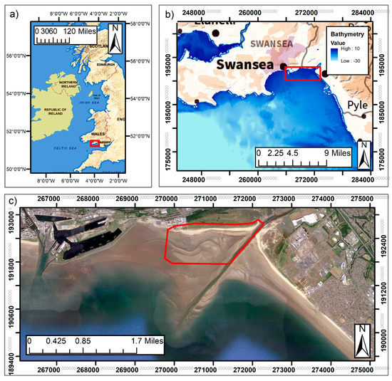
Figure 1.
(a) A map of Great Britain with the location of panel b marked in red; (b) The Swansea Bay area showing local bathymetry with the location of panel c marked in red; (c) An aerial photo showing the surroundings of Crymlyn Burrows with the drone survey area marked. Map contains OS data © Crown copyright and database right (2020), reproduced under Open Government Licence. Aerial imagery copyright 2020 Google; Data SIO, NOAA, US Navy, GEBCO.
Swansea Bay is an urbanized embayment in the Bristol Channel. It is a mega-tidal environment with a mean spring range of 8.46 m and a mean neap range of 4.03 m as reported by the National Tidal and Sea Level Facility gauge at Mumbles [64], which is on the western edge of Swansea Bay 9 km from the site. Consequently, there is also strong spring neap variation in residual tidal current speeds [65]. Prevailing winds are from the south west based on data extracted from the UK met office weather station the Mumbles Head for the duration of the drone surveys (Figure 2). Measurements from a Datawell Directional Waverider mkIII wave buoy deployed in water depths of 9 m LAT in the centre of Swansea Bay (51.5748N, 3.9115W) show prevailing wave directions are similar (Figure 2). There are several large offshore sandbanks in the vicinity of the study site [66,67,68] but these do not affect wave transformation between the offshore and study site; instead nearshore bathymetry is relatively uniform (Figure 1b). Intertidal bathymetry can be seen in Figure 1c; in the central portion of the beach, which equates to the western end of the dune system, is a series of crescentic intertidal bars which are believed to affect dune morphology [63]. Pye, et al. [63] postulate that small variation in intertidal morphology can lead to large variation in intertidal wave conditions.
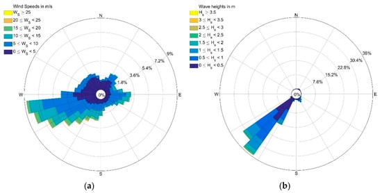
Figure 2.
(a) A wind rose taken from the Mumbles weather station, operated by the UK Meteorological Office; (b) A wave rose from a wave buoy situated in the centre of Swansea Bay. Data taken for the duration of the drone-based surveys (October 2018—December 2019).
2.2. Survey Methodology
Morphological surveys were conducted with a SenseFly eBee-RTK UAV; a light (<1 kg) fixed wing drone, launched by hand and powered by a single electric motor. Flights were pre-programmed in the Sensefly Emotion3 software and then, at site, flights ran on autopilot. Missions were run in RTK mode with network RTK corrections passed to the drone via a tablet linked to the Topnet-live system. A Sony WX 16MP camera, modified by Sensefly for drone use, was used to take images. Surveys between October 2018 and December 2019 are analyzed in this paper.
Area covered per flight was limited by battery endurance and the UK CAA visual line of sight regulation that limits drone distance from operator to 500 m. Therefore, four overlapping flights were flown to cover the area of interest which spanned the length of the dune system from MSL to inland of the frontal dunes (Figure 3). Lateral and longitudinal overlap was set to be 70–80%, dependent on flight conditions. Under stronger winds battery endurance required lesser overlap. Ground pixel distance was set at 0.03 m which resulted in a flight level of ~100 m above take-off level.
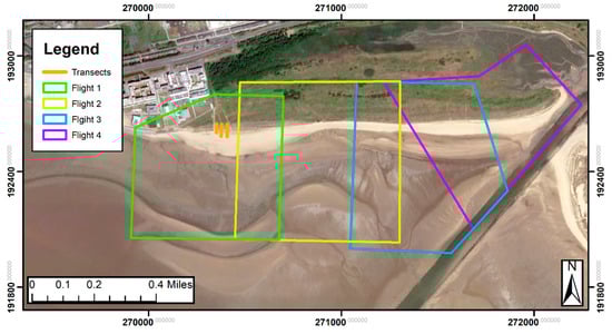
Figure 3.
A map showing the four overlapping flight areas used to cover the dune system and also the location of the three transects used to test vegetation removal method.
Variation in accuracy with increasing number of ground control points (GCPs) was tested to establish the appropriate number of GCPs to use. Table 1 shows mean absolute error between drone derived digital terrain map (DTM) and RTK-GPS surveyed points over the intertidal and non-vegetated supratidal area. It shows that increasing number of GCPs does not affect accuracy, due to the drone being equipped with RTK positioning. Based on this assessment, 4–6 ground control points consisting of black and white 24 cm quadrants were evenly spread about each flight area and surveyed using RTK-GPS prior to flying.

Table 1.
Mean absolute errors between RTK-GPS measured and drone derived elevations for a flight conducted with 80% overlap and varying numbers of GCPs used.
Initial SfM postprocessing was conducted in Pix4D, a well-known piece of photogrammetry software, to generate the point cloud and orthomosaics. The Pix4D approach to SfM is described in [69]. Subsequently, the point cloud was exported into CloudCompare, a point cloud processing software package [70], in order to denoise and down sample the data. Only the bare sand beach area was de-noised and down sampled because the three-dimensionality of the dune area meant that high resolution was required and defining spurious points without including valid point was unachievable. CloudCompare’s ‘Noise Filter’ was used to remove erroneous points from the point cloud: a local plane of radius 10 m was fitted to the point cloud around each point and then that point removed if it was more than 0.5 m from the plane. Down sampling was conducted by applying a minimum distance between points of 0.3 m; this second step was only conducted for areas of low morphological variability and was conducted to reduce the size of the point cloud which facilitates computationally efficient data analysis.
Vegetation points were removed from the point cloud using a colour-based discrimination between vegetation and sand. A two-layer feed forward neural network [71] was set up in Matlab to identify and remove vegetation points using RGB data from the point cloud. The network was trained using the scaled conjugate gradient method [72] on a subset of the data of known type (sand or vegetation). The authors have previously used a similar discrimination methodology successfully to distinguish between sand and mud [47].
Vegetated points were removed rather than lowered (as suggested by Bastos, et al. [62]) because of the difficulty in knowing variation in vegetation height over the larger study area. Finally, each point cloud was interpolated onto the same 0.5 m resolution regular grid to create a DTM from which further analysis was conducted. This approach was used because the automatic digital terrain map (DTM) creation in Pix4D was known to give poor results [73]. In order to validate the vegetation removal approach, three cross-shore profiles through the dune were collected and compared to the drone derived morphology. Points were taken both on bare sand and in vegetated sections, where care was taken to ensure the bare sand level was measured. Comparison between the RTK-measured profiles (locations shown in Figure 3), the drone derived profile including vegetation and the drone derived profile with vegetation removed is shown in Figure 4. Removing the vegetation points brings the drone derived profile closer to the actual bare earth profile. Table 2 shows the MAEs for the three profiles both with and without the vegetation points; removing vegetation reduces the MAE by over half compared to including vegetation. On average, the profiles with vegetation removed had a MAE of 0.087 m which is considered acceptable given the challenge of surveying the environment and given that even on open beach mean absolute error is between 0.05–0.06 m.
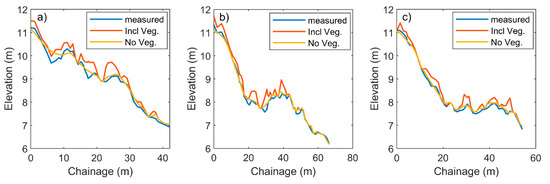
Figure 4.
Comparison between GPS measured bare earth profile and drone derived profiles with and without vegetation points included: (a) transect 1; (b) transect 2; (c) transect 3.
Table 2.
Mean absolute errors between RTK-GPS measured and drone derived elevations for the three transects over the frontal dune.
Consideration was given to volumetric changes to the frontal dune and upper intertidal beach. The frontal dune was defined as the area between highest astronomical tide and the frontal dune crest and the volume calculated as the volume of sediment above the lowest astronomical tide (LAT) level. The upper intertidal beach volume was defined as the volume, above LAT, between the mean sea level contour and the highest astronomical tide (HAT) contour.
2.3. Satellite Derived Intertidal Bar Locations
The drone derived morphology did not extend much below the mean sea level contour and therefore Sentinel-2 [74] satellite imagery was used to provide insights into intertidal bar migration. While quantitative sandbar volume is not achievable; qualitative information about sandbar shape and migration can be obtained and sandbar centroids used to estimate migration rates. Imagery was accessed using the CoastSat toolbox [75], which downloads imagery from Google Earth Engine [76] for specified regions. The focus of the toolbox is shoreline extraction but pre-proccessed RGB images prior to shoreline extraction are stored and it is these images that were considered here. Only images that were taken near low tide with minimal cloud cover were used in the analysis. Images were extracted between 01 January 2016 and 01 August 2020, with 30 suitable dates available.
The downloaded images had no further georeferencing than conducted by the provider [75]; therefore, in order to ensure all images were aligned as closely as possible, images were translated to match the first image based on pixels shifts that were calculated through cross correlation between images using a sub section of the image including fixed buildings as a template.
Sandbar locations were picked using image intensity contours: the concept being that sandbar crests will be drier and appear as higher intensity than the troughs. Prior to contour extraction, the images were transformed to greyscale; pixels outside the area of interest masked out; pixels within the area of interest contrast stretched to the 3rd and 98th percentile of intensity values in that region; and, images were smoothed using a circular averaging filter of radius 10 pixels. Due to variations in lighting and drying time between dates, the contrast level used to define the sand banks was not constant between dates but instead manually defined to best represent sandbar location and shape in each image. Intensity varied between 125 and 205 (from a range of 0 to 255). Centroids of individual sandbars were then calculated based on the contour lines.
2.4. Short Term Experiments on Wave Conditions Close to the Dune Line
To explore the importance of wave conditions on the longshore variation of dune response, piezoelectric pressure transducers (PTs) were deployed to measure high tide wave conditions over two storms coincident with spring tides: 13–16 January 2020 and 9–13 March 2020. High tide values are calculated as the average of the two values either side of high tide and results are presented as variation in high tide significant wave height and variation in wave spectra. Only high tide times were considered as this is when dune erosion by waves is most likely. Both storms were incident from the south west and significant wave heights measured at the Swansea Bay wave buoy peaked at 2.8 m for the first storm and 2.1 m for the second storm, albeit neither peak was coincident with high tide (Figure 5); this puts them above the 98th percentile for wave heights measured at the buoy (deployed since February 2018).
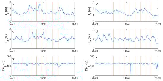
Figure 5.
Wave parameters (significant wave height (Hs), mean wave period (Tz), peak direction (Dirp) measured at the Swansea Bay waverider during the course of the two deployments: (a,c,e) deployment 1; (b,d,f) deployment 2. Blue lines indicate the wave parameters and orange lines the times of high tide.
RBR Solo D wave 16 transducers were used; these are commercially available pressure transducers that are commonly used in nearshore wave transformation studies (e.g., [77,78,79]). The pressure transducers were calibrated by the manufacturer prior to shipment and further user calibration is not recommended [80]. The instruments were set to measure pressure at 16 Hz for 8192 samples, (~8.5 m), every 30 min. Standard wave parameters, such as significant wave height and mean wave period, are automatically calculated by the instrument’s software. The process is: the raw timeseries data is demeaned and detrended (to remove atmospheric effects and tidal slope) before a direct Fourier transform used to convert to frequency space; frequencies greater than the max frequency and conjugate aliases are removed and then a frequency dependent attenuation correction applied before the data is re-transformed to a timeseries; then, this corrected dataset is then used to calculate mean period based on zero up-crossing and significant wave height based on the average of the highest 1/3 of waves in each record [81]. The burst data is also returned, and this was used to estimate wave spectra. Burst data was linearly detrended to remove tidal slope prior to estimation of the power spectral density. This was estimated using Welch’s overlapped segment averaging estimator with a Hamming window of length 1024 samples and with a 50% overlap.
Six PTs were deployed using helical sand anchors. The PTs were deployed level with the beach surface in a longshore line; with a longshore spacing of 200–300 m (Figure 6). The PTs were all deployed at the same beach surface elevation of 1.71 m ODN, with a standard deviation in vertical position of 0.02 m. This is close to mean high water neaps and hence data was returned every high tide. The longshore positions were kept the same for both experiments and are shown in Figure 6a. In this analysis, PTs were numbered from 1–6 going from west to east. Figure 6b shows cross-shore profiles of the mean beach surface (averaged over all drone surveys) between PT locations and the supratidal. It can be seen that for PTs 3–6, the profiles are similar: the slopes of the presented profile section ranges from 0.026–0.32 and the slope at HAT ranges from 0.097 to 0.145. PT 1 has shallower gradients (profile slope 0.023, slope at HAT 0.052). PT 2 has an overall gradient of 0.028 similar to PTs 3-6 but a shallower slope at HAT (0.057).
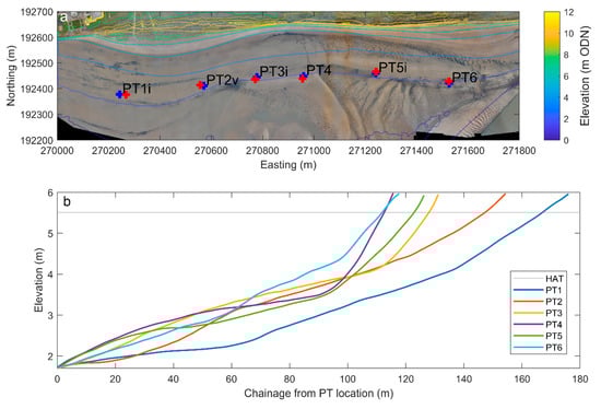
Figure 6.
(a) Locations of the six pressure transducers for deployment 1 (blue) and deployment 2 (red) overlain on an orthomosaic of the site with coloured contours showing the mean beach surface elevation; (b) cross-shore profiles of the mean beach surface from the location of each PT to an elevation of 6 m ODN.
Variation in wave spectra is considered using Goda’s peakedness parameter [82], Qp, which can be calculated as:
where m0 is the zero spectral moment, f is the frequency, and E is the spectral energy density. Larger vales of Qp indicate greater amounts of energy in the spectral peak.
3. Results
The results section is split into three parts: results for the morphological surveys; results for the intertidal sandbar evolution; and, results for the intertidal wave measurements.
3.1. Morphological Surveys
Figure 7 shows the mean morphology for the beach-dune system over the tested time period. Over the 2 km dune frontage there is a stark variation in the dune morphology. One can also notice differences in the intertidal morphology; the end of the crescentic intertidal bar is evident in the south-western corner of the data. Marked in Figure 7 are three dune subsections representative of the different morphotypes observed. Detailed plots of these areas are shown in Figure 8. Area 1 (Figure 8a,b) shows a healthy frontal dune, with the formation of a new dune ridge evident on the western portion. Over the studied period there has been a general accretion over the dune area; the slight erosion in the bottom left of the Figure is in the intertidal.
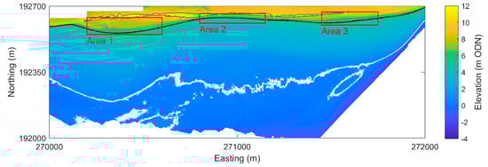
Figure 7.
A morphological map of the study area. The contours indicate the mean sea level contour (white), the highest astronomical tide contour (black) and a contour at 10.75 m ODN providing an indication of the frontal dune crest (grey). Red boxes indicate the areas displayed in greater detail.
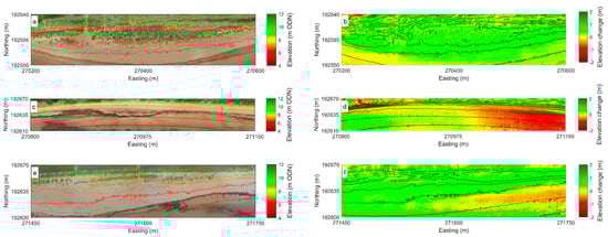
Figure 8.
(a) An orthomosaic of the first dune section (Area 1) with colored elevation contours at 1 m intervals; (b) change in elevation between first and last survey Figure 1. the same contours as (a) are displayed in black; (c,d) the same plots for Area 2; (e,f) the same plots for Area 3.
The second area (Figure 8c,d), shows are region of steeply cliffed dune morphology, this cliffed morphology has persisted since erosion during the extreme winter of December 2013–February 2014 [83]. Over the observation period, there was substantial erosion of the cliffed portion to the west of this section. There was also erosion at the dune toe throughout the section. To the east, one can see erosion had occurred at the top of the cliffed section and accretion in the middle, indicative of dune slumping.
Area 3, the eastern most section (Figure 8e,f), is an area of lower dunes. This area is generally accreting. There is clear evidence of protodunes in the orthomosaic imagery between 6–7 m ODN and a suggestion of a new dune line forming between the 7–9 m ODN contours (Figure 8e). The erosion that can be seen between eastings 271,600–271,750 m occurs around the level of highest astronomical tide but does not affect the main dune area. Also visible are diagonal stripes of erosion and accretion in the developing dune line which are parallel to the prevailing wind direction and are indicative of aeolian sand transport into this dune line.
To look at the broader scale evolution of the dune system, frontal dune volumes were calculated from the DSM for 100 m sections. These volumes and their cumulative changes are shown in Figure 9. Largest volumes are found to the western end of the dune system and lowest in the central portion. Overall, there has been an accretion in the west and in the east with erosion or lesser accretion in the centre. Substantial accretion occurs in the central portion during summer months, but this accretion is not persistent. The area of cumulative erosion between 271,600 and 271,900 is believed to be caused by supratidal beach erosion not the dune erosion (see Figure 8d).
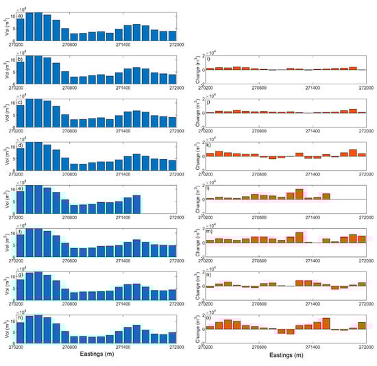
Figure 9.
Dune volumes for (a) 24 October 2018; (b) 16 November 2018; (c) 19 January 2019; (d) 25 February 2019; (e) 18 July 2019; (f) 28 August 2019; (g) 28 October 2019; (h) 17 December 2019; and cumulative change from the first survey for (i) 16 November 2018; (j) 19 January 2019; (k) 25 February 2019; (l) 18 July 2019; (m)28 August 2019; (n) 28 October 2019; (o) 17 December 2019.
In order to assess whether dune volumes and change in dune volumes were related to upper intertidal beach volumes, as has previously been suggested over shorter timescales (e.g., [29]), Figure 10 shows scatter plots of these parameters. There is no relationship between dune volume change and either upper intertidal beach volume or change in upper intertidal beach volume. There is a slight relationship between dune volume and beach volume: areas of large dune volume are not found where beach volumes are small. However, large beach volume does not imply large dune volume. Upper intertidal beach widths, between MSL and HAT, were also compared to dune volume and dune volume change (not shown); these showed very similar patterns to the upper intertidal beach volume.
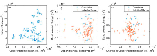
Figure 10.
Scatter plots of: (a) dune volume against beach volume above MSL; (b) dune volume change against beach volume above MSL; (c) dune volume change against beach volume change. For panels b&c, both change between individual surveys and cumulative change is presented.
3.2. Sattelite Derived Intertidal Bar Migration
Figure 11 shows a subset of eight of the satellite images with the intensity derived shapes and locations for the two main crescentic bars and key secondary bars overlaid. The two main crescentic sandbars migrate northward (onshore) with the southern bar growing as it migrates onshore and the northern bar getting smaller. Towards the end of the image sequence (Figure 11g) the two bars merge. In Figure 11a,b, while not ringed in orange, one can also note another bar welding to the high-tide shoreface in front of dune Section 1 (Figure 7 and Figure 8). As well as the two main crescentic bars, one can see the eastward longshore migration of secondary bars that episodically detach from the eastern end of the crescentic bar. One such detachment initiates in Figure 11c, where a dewatering channel (darker in the grayscale image) seems to cut through the crescentic bar. The detached portion moves eastward as it continues to migrate onshore, before reaching the inner intertidal shoreface near dune Section 3 (Figure 7 and Figure 8). Noticeable as well in the greyscale images, but not highlighted by the contours, is a large transverse sandbar associated with the estuary mouth.
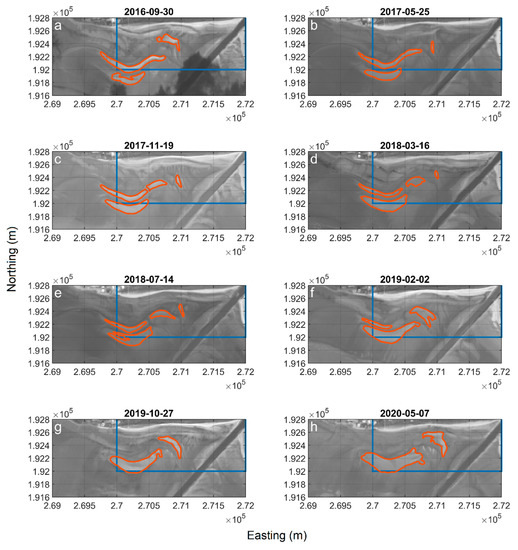
Figure 11.
Grayscale images of the intertidal at low tide with key sandbars determined from grayscale intensity contours marked in orange, and the area of maximum drone flight coverage marked in blue, for the dates (a) 30 September 2016, (b) 25 May 2017, (c) 19 November 2017, (d) 16 March 2018, (e) 14 July 2018, (f) 2 February 2019, (g) 27 October 2019, (h) 7 May 2020.
Migration of sandbar centroid positions is shown in Figure 12. Figure 12a shows the cross shore migration of the two crescentic bars. For the further offshore bar, migration is largely constant with linear fitting giving a rate of 0.2 m/day. For the further onshore bar, linear fitting gives a migration rate of 0.1 m/day; however, visually, it looks like the bar centroid migrates at a similar rate to the offshore bar until 2018 when its migration rate slows. Figure 12b shows the episodically detached smaller bars can migrate for several hundred meters in a longshore direction
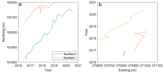
Figure 12.
Migration of sandbar centroids: (a) cross-shore migration of the two main crescentic sand bars; (b) longshore migration rates of the smaller sandbars that detach from the cresenetic bars.
3.3. Short Term Wave Experiments
Figure 13 shows high tide significant wave heights for the 6 PTs over successive high tides for both deployments. Wave heights are shown as percentage of the maximum significant wave height recorded by the pressure transducers. Waves were not breaking at the pressure transducers for any of the high tides based on the critical threshold for wave breaking γb of:
where h is the water depth and H is the significant wave height at a given point. While equations and values for γb can vary a lot (e.g., [84]), in this study high tide values of γb typically exceeded 2 so waves were clearly not breaking.
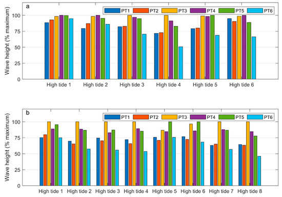
Figure 13.
High tide significant wave heights, presented as percentages of the maximum measured for each high tide, for the 6 pressure transducers (PTs), PT1 in the west to PT6 in the east: (a) deployment 1; (b) deployment 2.
It can been seen that there is substantial longshore change in significant wave heights; for deployment one, this ranged from a maximum 11% reduction (high tide 1) to a maximum 50% reduction (high tide 4) and for deployment 2, the maximum change ranged from 25% (high tide 1) to 54% (high tide 8). In real values, this equated to reductions of up to 0.65 m from the maximum significant wave height recorded by the pressure transducers at a given time (see Table 3 and Table 4). Significance testing of these reductions using a two-sample t-test at the 95% level showed that for deployment 1, the reductions of PT1, PT2 & PT6 are statistically similar and statistically different to PT 3, PT4, & PT5; with PT3, PT4 & PT5 also statistically the same. Broadly the same pattern of significance is shown for deployment 2, but PT3 and P4 are also statistically different. While there is variation in location of the highest significant wave heights for each high tide, significant wave heights are constantly higher at pressure transducers 3, 4 and 5 (central pressure transducers) compared to pressure transducers 1 and 2 (western) and pressure transducer 6 (easternmost). For deployment 1, the only time that this is not evident is high tide 6; during this time only PT6 shows a substantial reduction. This difference can be explained by the wave direction which comes from the SSE rather than the predominant SW direction. High tide one shows least longshore variation in significant wave height and high tide 4 the most; peak wave periods (not shown) are 13.3 s for high tide 4; over double the high tide 1 value (6.5 s) which may explain the difference. There is less variability in the variation for deployment 2; during this deployment mean wave periods were consistent (within 1 s) and there was minimal change in wave direction (13 degrees difference).
Table 3.
Longshore significant wave height reductions (m) compared to maximum measured significant wave height for deployment 1.
Table 4.
Longshore significant wave height reductions (m) compared to maximum measured significant wave height for deployment 2.
Some longshore variation in spectral shape was also noted; Figure 14 shows spectra that have been normalized by the total energy (such that the area under each normalized spectrum is equal to 1) for the two deployments. It can be seen that, at some times, more energy is concentrated in the spectral peak for PTs 2,3 and 4 compared to the others; however, in general the envelope of spectra are similar. This concentration of energy is less noticeable for deployment 2. To assess this, Equation (1) was used to calculated Goda’s peakedness parameter Qp (Table 5). In general, the values are low suggesting all spectra are quite wide banded. For deployment one, values of Qp are slightly higher in the middle but mean values are largely within one standard deviation of each other. For deployment two, the patterns in Qp are less clear with higher values for PT3 and PT5 and the other values being similar. Significance testing using a two-sample t-test showed that there was no statistical difference at the 95% in mean values of Qp for either deployment. Therefore, it is believed limited import can be attributed to spectral differences.
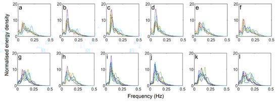
Figure 14.
Normalised wave spectra averaged over each high tide at the 6 pressure transducers for deployment one (a–f) and deployment 2 (g–l). PTs are displayed from west to east; PT1 is the first column (a,g) through to PT6 the last column (f,l). Different colours indicate different high tides, but it is the envelope of spectral shapes rather than the individual spectra which should be considered.
Table 5.
Mean and standard deviation of Goda’s peakedness parameter, Qp, for both deployments.
Longshore variation in high tide water level was also tested. Over both deployments there was a slope to the water level with lowest values in the west (PT1) and higher values in the east (PT5 & PT6); however, the differences were small. For the first deployment the maximum difference between PTs was 0.12 m and for the second deployment maximum difference was 0.06 m. Moreover, these maximum differences were at the eastern end of the study site, in front of dune area C (Figure 7 and Figure 10), whereas in front of the eroding section (PT3 and PT4) differences were less than 0.03 m above water levels at PT1. Given that the vertical error in the RTK-GPS is ~0.02 m, longshore differences in water level cannot explain the observed differences in dune morphotype and evolution.
4. Discussion
Morphological surveys showed that there were a wide variety of dune morphotypes and behaviours over a 2 km section of dune frontage. Two factors were considered to explain this variation: the role of intertidal bar migration in onshore sediment supply and the longshore variation in nearshore hydrodynamic parameters.
Compared to regional scale studies that found variation in water level more important than wave height in determining longshore variation in dune erosion [20,32], over the smaller scale of this site, water level variation was not found to match areas of erosion. Statistically significant longshore variation in significant wave height was observed with larger significant wave heights fronting areas of erosion. The areas of lower significant wave heights were found in areas protected by the crescentic bars to the west and by a transverse bar associated with the estuary to the east. Therefore, this study corroborates the postulation of Pye, et al. [63], that intertidal bars affect dune erosion at the site by affecting wave dissipation. On an embayment scale, Splinter, et al. [29] find that despite significant alongshore variation in wave height, these variations do not match areas of increased erosion. Splinter, et al. [29] assessed a microtidal wave-exposed embayment and hence this difference highlights how environmental setting is important in defining key parameters. One of the goals of the pressure transducer deployment was to establish whether longshore variation in wave spectral shape caused by variation in intertidal wave transformation might have been important in dictating dune response. Visually, it looked like spectra recorded behind the crescentic bars had less energy in the spectral peak, with energy shifted to higher frequencies; this would have affected swash zone processes and was postulated to be caused by frequency shifting over the intertidal bar. However, testing using Goda’s peakedness parameter showed there was no statistical significance in this longshore variation.
Significant wave heights and spectra are considered rather than using these to compute wave runup for two main reasons: firstly, run-up formula predominantly use deep water wave heights and hence calculating from the measured intertidal values is not achievable; secondly, there is a large variation in the results of these formulae and hence uncertainty in which formula is appropriate [85,86]. The beach profiles between the PT location and the dune area (Figure 6) further enhance the effect that differences in significant wave heights would have on dune erosion: the profile gradients for PT1 and PT2 (where significant wave heights are lower) are shallower and hence would have lesser predicted run-up values for many formulas [87] even if wave heights were similar. In contrast, gradients are similar for profiles at PTs 3–6 and hence one would expect similar wave run-up statistics at these locations for the same wave conditions. It should be noted that the exact influence of beach slope on run-up is uncertain and Ruessink, et al. [88] suggest that on dissipative beaches, beach slope does not affect runup values.
Researchers have demonstrated the importance of antecedent morphology on storm impact [20,89] and storm recovery [90]. Relationships between dune volume or dune volume change and upper intertidal beach volume or width were not found, suggesting it is less important at Crymlyn Burrows. This is in contrast to studies ranging from embayment [29] to regional scales [20,32]. It is postulated that the difference may be related to the lack of supra-tidal beach between the HAT level and the dunefoot at the studied site; lack of supratidal beach means that wave coincident with spring high tide will impact the dunefoot all along the studied dune system. The importance of the shape of antecedent morphology on longshore variation in dune evolution has been raised by Brodie, et al. [30]. This has not been assessed here but it is postulated that antecedent morphology could play an important role in the amount of aeolian sediment trapped at a given section for Crymlyn Burrows. The prevailing wind direction is from the WSW which is almost parallel to the dune line. Therefore, once a section has become eroded and cliffed there is little to trap the aeolian transport of sand; hence, post-storm morphology may be important in dictating variation in subsequent recovery at this site. Over recent years, attention has been given to whether dunes systems are becoming “over-vegetated” [4,5,6]; it is postulated that this phenomenon may exacerbate the role of antecedent morphology. Vegetation stabilizes the dune which increases the angle of repose and reduces dune slumping; this means that cliffing persists longer than it would for less vegetated dunes. However, it is hard to disentangle the various factors because it is the longshore variation in wave heights that are likely to have caused longshore variation in antecedent morphology.
One aim of this study was to consider how the megatidal environment influenced dune evolution. This study has demonstrated that the three-dimensionality of intertidal morphology controls the longshore variation in dune response. It is known that tidal range affects modal beach morphology [91,92] and hence would affect the type of intertidal three-dimensionality and how it interacts with the dune system. Here, the multiple intertidal bar (MITB) morphotype causes the longshore variation in dune evolution; Biausque, et al. [93] show that while MITBs have been identified in areas with tidal ranges of 3 m, they are much more common in tidal ranges over about 6 m (macrotidal and above). Megatidal regions often display increased importance of tidal currents and it is postulated that estuary directed currents may play a role in the longshore migration of the smaller sandbars noted at this site; hence in a region of lower tidal range there might be lesser longshore variation in onshore sediment supply.
5. Conclusions
A fixed wing drone, the Sensefly Ebee-RTK is used to map coastal dunes at a UK study site. The method is shown to be sufficiently accurate (MAE = 0.05 m on bare sand; 0.09 m on vegetated areas) and able to identify dune features and changes over a range of scales.
Coastal dunes at the site are shown to exhibit significantly different morphology and evolution over short longshore distances (~500 m). Areas of dunes at the extremity of the study area exhibit a healthy morphology of fore dunes and proto dunes. These areas are accreting over the surveyed year. In the central portion, the dunes are in a persistently cliffed state with erosive or static volumetric changes.
Intertidal bar morphology and migration are examined using Sentinel-2 satellite imagery. To the western portion of the study area, large crescentic intertidal bars are present which migrate onshore. Episodically, these bars weld to the high-tide beachface which would provide a reservoir of sediment to nourish the dunes. There is also episodic detachment of lenses of sediment from the bars which migrate eastward and nourish the eastern portion of the study site. There is not obvious transfer of sediment from the bars to the central (eroding) section of the dune.
Beachface mounted pressure transducers are used to explore whether longshore variation in water level and wave conditions can explain the variation in dune morphodynamics. Water level variation does not explain variation in dune response, in contrast to previous studies; nor does longshore variation in spectral shape which was shown to be insignificant. Statistically significant longshore differences in significant wave heights are noted: larger significant wave heights are present in front of the cliffed, eroding, section and lower significant wave heights behind the section protected by the crescentic bars.
This work shows that variation in three-dimensional intertidal beach morphology has a significant impact on dune morphology and evolution both through longshore variation in sediment supply to the dune and by causing variation in wave heights incident to the dune.
Author Contributions
Conceptualization, I.F. formal analysis, I.F. and J.H.-C.; funding acquisition, I.M., H.K. and D.E.R.; methodology, I.F.; Supervision, I.M. and D.E.R.; writing—original draft, I.F.; writing—review and editing, I.F., J.H.-C., I.M., H.K. and D.E.R. All authors have read and agreed to the published version of the manuscript.
Funding
This work was conducted through the financial support of the Welsh European Funding Office EU ERDF project Seacams2.
Acknowledgments
The authors wish to thank staff and students of Swansea University who provided additional fieldwork help: Anouska Mendzil, Georgie Blow, Henry Miller, Yunzhu Yin, Hazel Wakefield.
Conflicts of Interest
The authors declare no conflict of interest.
References
- Drius, M.; Jones, L.; Marzialetti, F.; de Francesco, M.C.; Stanisci, A.; Carranza, M.L. Not just a sandy beach. The multi-service value of Mediterranean coastal dunes. Sci. Total Environ. 2019, 668, 1139–1155. [Google Scholar] [CrossRef] [PubMed]
- Sigren, J.M.; Figlus, J.; Highfield, W.; Feagin, R.A.; Armitage, A.R. The Effects of Coastal Dune Volume and Vegetation on Storm-Induced Property Damage: Analysis from Hurricane Ike. J. Coast. Res. 2018, 34, 164–173. [Google Scholar] [CrossRef]
- Gao, J.J.; Kennedy, D.M.; Konlechner, T.M. Coastal dune mobility over the past century: A global review. Progress Phys. Geogr. -Earth Environ. 2020. [Google Scholar] [CrossRef]
- Jackson, D.W.T.; Costas, S.; González-Villanueva, R.; Cooper, A. A global ‘greening’ of coastal dunes: An integrated consequence of climate change? Glob. Planet. Chang. 2019, 182, 103026. [Google Scholar] [CrossRef]
- Creer, J.; Litt, E.; Ratcliffe, J.; Rees, S.; Thomas, N.; Smith, P. A comment on some of the conclusions made by Delgado-Fernandez et al. (2019). “Is ‘re-mobilisation’ nature conservation or nature destruction? A commentary”. J. Coast. Conserv. 2020, 24, 29. [Google Scholar] [CrossRef]
- Delgado-Fernandez, I.; Davidson-Arnott, R.G.D.; Hesp, P.A. Is ‘re-mobilisation’ nature restoration or nature destruction? A commentary. J. Coast. Conserv. 2019, 23, 1093–1103. [Google Scholar] [CrossRef]
- Castelle, B.; Laporte-Fauret, Q.; Marieu, V.; Michalet, R.; Rosebery, D.; Bujan, S.; Lubac, B.; Bernard, J.B.; Valance, A.; Dupont, P.; et al. Nature-Based Solution along High-Energy Eroding Sandy Coasts: Preliminary Tests on the Reinstatement of Natural Dynamics in Reprofiled Coastal Dunes. Water 2019, 11, 2518. [Google Scholar] [CrossRef]
- Ruessink, B.G.; Arens, S.M.; Kuipers, M.; Donker, J.J.A. Coastal dune dynamics in response to excavated foredune notches. Aeolian Res. 2018, 31, 3–17. [Google Scholar] [CrossRef]
- Anthony, E.J.; Vanhee, S.; Ruz, M.H. Short-term beach-dune sand budgets on the north sea coast of France: Sand supply from shoreface to dunes, and the role of wind and fetch. Geomorphology 2006, 81, 316–329. [Google Scholar] [CrossRef]
- Bauer, B.O.; Davidson-Arnott, R.G.D. A general framework for modeling sediment supply to coastal dunes including wind angle, beach geometry, and fetch effects. Geomorphology 2003, 49, 89–108. [Google Scholar] [CrossRef]
- Jackson, D.W.T.; Beyers, M.; Delgado-Fernandez, I.; Baas, A.C.W.; Cooper, A.J.; Lynch, K. Airflow reversal and alternating corkscrew vortices in foredune wake zones during perpendicular and oblique offshore winds. Geomorphology 2013, 187, 86–93. [Google Scholar] [CrossRef]
- Hesp, P.A.; Smyth, T.A.G. Surfzone-Beach-Dune interactions: Flow and Sediment Transport across the Intertidal Beach and Backshore. J. Coast. Res. 2016, 8–12. [Google Scholar] [CrossRef]
- Nordstrom, K.F.; Jackson, N.L. Offshore aeolian sediment transport across a human-modified foredune. Earth Surf. Process. Landf. 2018, 43, 195–201. [Google Scholar] [CrossRef]
- Nordstrom, K.F.; Bauer, B.O.; Davidson-Arnott, R.G.D.; Gares, P.A.; Carter, R.W.G.; Jackson, D.W.T.; Sherman, D.J. Offshore Aeolian Transport Across a Beach: Carrick Finn Strand, Ireland. J. Coast. Res. 1996, 12, 664–672. [Google Scholar]
- Montreuil, A.L.; Bullard, J.E. Aeolian dune development on a macro-tidal coast with a complex wind regime, Lincolnshire coast, UK. J. Coast. Res. 2011, 64, 269–272. [Google Scholar]
- Nordstrom, K.F.; Gamper, U.; Fontolan, G.; Bezzi, A.; Jackson, N.L. Characteristics of Coastal Dune Topography and Vegetation in Environments Recently Modified Using Beach Fill and Vegetation Plantings, Veneto, Italy. Environ. Manag. 2009, 44, 1121–1135. [Google Scholar] [CrossRef]
- Jackson, N.L.; Nordstrom, K.F. Aeolian sediment transport and landforms in managed coastal systems: A review. Aeolian Res. 2011, 3, 181–196. [Google Scholar] [CrossRef]
- De Battisti, D.; Griffin, J.N. Below-ground biomass of plants, with a key contribution of buried shoots, increases foredune resistance to wave swash. Ann. Bot. 2020, 125, 325–334. [Google Scholar] [CrossRef]
- Beuzen, T.; Goldstein, E.B.; Splinter, K. Ensemble models from machine learning: An example of wave runup and coastal dune erosion. Nat. Hazards Earth Syst. Sci. 2019, 19, 2295–2309. [Google Scholar] [CrossRef]
- Beuzen, T.; Harley, M.D.; Splinter, K.D.; Turner, I.L. Controls of Variability in Berm and Dune Storm Erosion. J. Geophys. Res. -Earth Surf. 2019, 124, 2647–2665. [Google Scholar] [CrossRef]
- Bryant, D.B.; Bryant, M.A.; Sharp, J.A.; Bell, G.L.; Moore, C. The response of vegetated dunes to wave attack. Coast. Eng. 2019, 152. [Google Scholar] [CrossRef]
- Crapoulet, A.; Hequette, A.; Marin, D.; Levoy, F.; Bretel, P. Variations in the response of the dune coast of northern France to major storms as a function of available beach sediment volume. Earth Surf. Process. Landf. 2017, 42, 1603–1622. [Google Scholar] [CrossRef]
- Muller, H.; van Rooijen, A.; Idiert, D.; Pedreros, R.; Rohmer, J. Assessing Storm Impact on a French Coastal Dune System Using Morphodynamic Modeling. J. Coast. Res. 2017, 33, 254–272. [Google Scholar] [CrossRef]
- Pye, K.; Blott, S.J. Assessment of beach and dune erosion and accretion using LiDAR: Impact of the stormy 2013-14 winter and longer term trends on the Sefton Coast, UK. Geomorphology 2016, 266, 146–167. [Google Scholar] [CrossRef]
- van Thiel de Vries, J.S.M.; van Gent, M.R.A.; Walstra, D.J.R.; Reniers, A.J.H.M. Analysis of dune erosion processes in large-scale flume experiments. Coast. Eng. 2008, 55, 1028–1040. [Google Scholar] [CrossRef]
- Aagaard, T.; Davidson-Arnott, R.; Greenwood, B.; Nielsen, J. Sediment supply from shoreface to dunes: Linking sediment transport measurements and long-term morphological evolution. Geomorphology 2004, 60, 205–224. [Google Scholar] [CrossRef]
- Cohn, N.; Hoonhout, B.M.; Goldstein, E.B.; de Vries, S.; Moore, L.J.; Vinent, O.D.; Ruggiero, P. Exploring Marine and Aeolian Controls on Coastal Foredune Growth Using a Coupled Numerical Model. J. Mar. Sci. Eng. 2019, 7, 13. [Google Scholar] [CrossRef]
- Cohn, N.; Ruggiero, P.; de Vries, S.; Kaminsky, G.M. New Insights on Coastal Foredune Growth: The Relative Contributions of Marine and Aeolian Processes. Geophys. Res. Lett. 2018, 45, 4965–4973. [Google Scholar] [CrossRef]
- Splinter, K.D.; Kearney, E.T.; Turner, I.L. Drivers of alongshore variable dune erosion during a storm event: Observations and modelling. Coast. Eng. 2018, 131, 31–41. [Google Scholar] [CrossRef]
- Brodie, K.; Conery, I.; Cohn, N.; Spore, N.; Palmsten, M. Spatial Variability of Coastal Foredune Evolution, Part A: Timescales of Months to Years. J. Mar. Sci. Eng. 2019, 7, 124. [Google Scholar] [CrossRef]
- Spencer, T.; Brooks, S.M.; Evans, B.R.; Tempest, J.A.; Möller, I. Southern North Sea storm surge event of 5 December 2013: Water levels, waves and coastal impacts. Earth-Sci. Rev. 2015, 146, 120–145. [Google Scholar] [CrossRef]
- Héquette, A.; Ruz, M.-H.; Zemmour, A.; Marin, D.; Cartier, A.; Sipka, V. Alongshore Variability in Coastal Dune Erosion and Post-Storm Recovery, Northern Coast of France. J. Coast. Res. 2019, 88, 25–45. [Google Scholar] [CrossRef]
- Levoy, F.; Anthony, E.J.; Monfort, O.; Larsonneur, C. The morphodynamics of megatidal beaches in Normandy, France. Mar. Geol. 2000, 171, 39–59. [Google Scholar] [CrossRef]
- Levoy, F.; Monfort, O.; Larsonneur, C. Hydrodynamic variability on megatidal beaches, Normandy, France. Cont. Shelf Res. 2001, 21, 563–586. [Google Scholar] [CrossRef]
- Dashtgard, S.E.; MacEachern, J.A.; Frey, S.E.; Gingras, M.K. Tidal effects on the shoreface: Towards a conceptual framework. Sediment. Geol. 2012, 279, 42–61. [Google Scholar] [CrossRef]
- Karunarathna, H.; Brown, J.; Chatzirodou, A.; Dissanayake, P.; Wisse, P. Multi-timescale morphological modelling of a dune-fronted sandy beach. Coast. Eng. 2018, 136, 161–171. [Google Scholar] [CrossRef]
- Goncalves, J.A.; Henriques, R. UAV photogrammetry for topographic monitoring of coastal areas. ISPRS J. Photogramm. Remote Sens. 2015, 104, 101–111. [Google Scholar] [CrossRef]
- Guillot, B.; Pouget, F. Uav Application In Coastal Environment, Example Of The Oleron Island For Dunes And Dikes Survey. In Isprs Geospatial Week 2015; Mallet, C., Paparoditis, N., Dowman, I., Elberink, S.O., Raimond, A.M., Sithole, G., Rabatel, G., Rottensteiner, F., Briottet, X., Christophe, S., et al., Eds.; ISPRS: La Grande Motte, France, 2015; Volume 40-3, pp. 321–326. [Google Scholar]
- Mancini, F.; Dubbini, M.; Gattelli, M.; Stecchi, F.; Fabbri, S.; Gabbianelli, G. Using Unmanned Aerial Vehicles (UAV) for High-Resolution Reconstruction of Topography: The Structure from Motion Approach on Coastal Environments. Remote Sens. 2013, 5, 6880–6898. [Google Scholar] [CrossRef]
- Turner, I.L.; Harley, M.D.; Drummond, C.D. UAVs for coastal surveying. Coast. Eng. 2016, 114, 19–24. [Google Scholar] [CrossRef]
- Brunier, G.; Michaud, E.; Fleury, J.; Anthony, E.J.; Morvan, S.; Gardel, A. Assessing the relationship between macro-faunal burrowing activity and mudflat geomorphology from UAV-based Structure-from-Motion photogrammetry. Remote Sens. Environ. 2020, 241. [Google Scholar] [CrossRef]
- de Sa, N.C.; Castro, P.; Carvalho, S.; Marchante, E.; Lopez-Nunez, F.A.; Marchante, H. Mapping the Flowering of an Invasive Plant Using Unmanned Aerial Vehicles: Is There Potential for Biocontrol Monitoring? Front. Plant Sci. 2018, 9. [Google Scholar] [CrossRef] [PubMed]
- Lin, Y.C.; Cheng, Y.T.; Zhou, T.; Ravi, R.; Hasheminasab, S.M.; Flatt, J.E.; Troy, C.; Habib, A. Evaluation of UAV LiDAR for Mapping Coastal Environments. Remote Sens. 2019, 11, 2893. [Google Scholar] [CrossRef]
- Nolet, C.; van Puijenbroek, M.; Suomalainen, J.; Limpens, J.; Riksen, M. UAV-imaging to model growth response of marram grass to sand burial: Implications for coastal dune development. Aeolian Res. 2018, 31, 50–61. [Google Scholar] [CrossRef]
- van Puijenbroek, M.E.B.; Nolet, C.; de Groot, A.V.; Suomalainen, J.M.; Riksen, M.; Berendse, F.; Limpens, J. Exploring the contributions of vegetation and dune size to early dune development using unmanned aerial vehicle (UAV) imaging. Biogeosciences 2017, 14, 5533–5549. [Google Scholar] [CrossRef]
- Suo, C.; McGovern, E.; Gilmer, A. Coastal Dune Vegetation Mapping Using a Multispectral Sensor Mounted on an UAS. Remote Sens. 2019, 11, 1814. [Google Scholar] [CrossRef]
- Fairley, I.; Mendzil, A.; Togneri, M.; Reeve, D.E. The Use of Unmanned Aerial Systems to Map Intertidal Sediment. Remote Sens. 2018, 10, 1918. [Google Scholar] [CrossRef]
- Laporte-Fauret, Q.; Marieu, V.; Castelle, B.; Michalet, R.; Bujan, S.; Rosebery, D. Low-Cost UAV for High-Resolution and Large-Scale Coastal Dune Change Monitoring Using Photogrammetry. J. Mar. Sci. Eng. 2019, 7, 63. [Google Scholar] [CrossRef]
- Andriolo, U.; Gonçalves, G.; Sobral, P.; Fontán-Bouzas, Á.; Bessa, F. Beach-dune morphodynamics and marine macro-litter abundance: An integrated approach with Unmanned Aerial System. Sci. Total Environ. 2020, 749, 141474. [Google Scholar] [CrossRef]
- Taddia, Y.; Stecchi, F.; Pellegrinelli, A. Coastal Mapping Using DJI Phantom 4 RTK in Post-Processing Kinematic Mode. Drones 2020, 4, 9. [Google Scholar] [CrossRef]
- Lim, M.; Dunning, S.A.; Burke, M.; King, H.; King, N. Quantification and implications of change in organic carbon bearing coastal dune cliffs: A multiscale analysis from the Northumberland coast, UK. Remote Sens. Environ. 2015, 163, 1–12. [Google Scholar] [CrossRef]
- Casella, E.; Drechsel, J.; Winter, C.; Benninghoff, M.; Rovere, A. Accuracy of sand beach topography surveying by drones and photogrammetry. Geo-Mar. Lett. 2020, 40, 255–268. [Google Scholar] [CrossRef]
- Conlin, M.; Cohn, N.; Ruggiero, P. A Quantitative Comparison of Low-Cost Structure from Motion (SfM) Data Collection Platforms on Beaches and Dunes. J. Coast. Res. 2018, 34, 1341–1357. [Google Scholar] [CrossRef]
- Moloney, J.G.; Hilton, M.J.; Sirguey, P.; Simons-Smith, T. Coastal Dune Surveying Using a Low-Cost Remotely Piloted Aerial System (RPAS). J. Coast. Res. 2018, 34, 1244–1255. [Google Scholar] [CrossRef]
- Pagan, J.I.; Banon, L.; Lopez, I.; Banon, C.; Aragones, L. Monitoring the dune-beach system of Guardamar del Segura (Spain) using UAV, SfM and GIS techniques. Sci. Total Environ. 2019, 687, 1034–1045. [Google Scholar] [CrossRef]
- Duffy, J.P.; Shutler, J.D.; Witt, M.J.; DeBell, L.; Anderson, K. Tracking Fine-Scale Structural Changes in Coastal Dune Morphology Using Kite Aerial Photography and Uncertainty-Assessed Structure-from-Motion Photogrammetry. Remote Sens. 2018, 10, 1494. [Google Scholar] [CrossRef]
- Guisado-Pintado, E.; Jackson, D.W.T.; Rogers, D. 3D mapping efficacy of a drone and terrestrial laser scanner over a temperate beach-dune zone. Geomorphology 2019, 328, 157–172. [Google Scholar] [CrossRef]
- Guillot, B.; Castelle, B.; Marieu, V.; Bujan, S.; Rosebery, D. UAV monitoring of 3-year Foredune Partial Recovery from a Severe Winter: Truc Vert Beach, SW France. J. Coast. Res. 2018, 85, 276–280. [Google Scholar] [CrossRef]
- Scarelli, F.M.; Cantelli, L.; Barboza, E.G.; Rosa, M.; Gabbianelli, G. Natural and Anthropogenic Coastal System Comparison Using DSM from a Low Cost UAV Survey (Capao Novo, RS/Brazil). J. Coast. Res. 2016, 75, 1232–1236. [Google Scholar] [CrossRef]
- De Giglio, M.; Greggio, N.; Goffo, F.; Merloni, N.; Dubbini, M.; Barbarella, M. Comparison of Pixel- and Object-Based Classification Methods of Unmanned Aerial Vehicle Data Applied to Coastal Dune Vegetation Communities: Casal Borsetti Case Study. Remote Sens. 2019, 11, 1416. [Google Scholar] [CrossRef]
- Takayama, N.; Kimura, R.; Liu, J.Q.; Moriyama, M. Long-term spatial distribution of vegetation and sand movement following the commencement of landscape conservation activities to curb grassland encroachment at the Tottori Sand Dunes natural monument (Vegetation and sand movement in the Tottori Sand Dunes). Int. J. Remote Sens. 2020, 41, 3070–3094. [Google Scholar] [CrossRef]
- Bastos, A.P.; Lira, C.P.; Calvao, J.; Catalao, J.; Andrade, C.; Pereira, A.J.; Taborda, R.; Rato, D.; Pinho, P.; Correia, O. UAV Derived Information Applied to the Study of Slow-changing Morphology in Dune Systems. J. Coast. Res. 2018. [Google Scholar] [CrossRef]
- Pye, K.; Blott, S.J. Crymlyn Burrows & Baglan Burrows: Geomorphological Assessment; Neath Port Talbot Council, Ed.; KPal: Wokingham, UK, 2014. [Google Scholar]
- NTSLF. Mumbles Tide Gauge Site. Available online: https://www.ntslf.org/tgi/portinfo?port=Mumbles (accessed on 1 March 2020).
- Uncles, R.J. Physical properties and processes in the Bristol Channel and Severn Estuary. Mar. Pollut. Bull. 2010, 61, 5–20. [Google Scholar] [CrossRef] [PubMed]
- Fairley, I.; Masters, I.; Karunarathna, H. Numerical modelling of storm and surge events on offshore sandbanks. Mar. Geol. 2016, 371, 106–119. [Google Scholar] [CrossRef]
- Pattiaratchi, C.; Collins, M. Wave influence on coastal sand transport paths in a tidally dominated environment. Ocean Shorel. Manag. 1988, 11, 449–465. [Google Scholar] [CrossRef]
- Pattiaratchi, C.; Collins, M. Mechanisms for linear sandbank formation and maintenance in relation to dynamical oceanographic observations. Prog. Oceanogr. 1987, 19, 117–176. [Google Scholar] [CrossRef]
- Küng, O.; Strecha, C.; Beyeler, A.; Zufferey, J.C.; Floreano, D.; Fua, P.; Gervaix, F. The Accuracy Of Automatic Photogrametric Techniques On Ultra-light UAV Imagery. Int. Arch. Photogramm. Remote Sens. Spat. Inf. Sci. 2012, XXXVIII-1/C22, 125–130. [Google Scholar] [CrossRef]
- v2.10, C. Available online: http://www.cloudcompare.org/ (accessed on 1 July 2018).
- Svozil, D.; Kvasnicka, V.; Pospichal, J.í. Introduction to multi-layer feed-forward neural networks. Chemom. Intell. Lab. Syst. 1997, 39, 43–62. [Google Scholar] [CrossRef]
- Møller, M.F. A scaled conjugate gradient algorithm for fast supervised learning. Neural Netw. 1993, 6, 525–533. [Google Scholar] [CrossRef]
- Fairley, I.; Mendzil, A.; Reeve, D.E. Monitoring of Intertidal Morphodynamics around Swansea Bay; SC2-R&D-S08; Swansea University: Swansea, UK, 2018; p. 39. [Google Scholar]
- ESA. Sentinal-2. Available online: https://sentinel.esa.int/web/sentinel/missions/sentinel-2 (accessed on 14 October 2020).
- Vos, K.; Splinter, K.D.; Harley, M.D.; Simmons, J.A.; Turner, I.L. CoastSat: A Google Earth Engine-enabled Python toolkit to extract shorelines from publicly available satellite imagery. Environ. Model. Softw. 2019, 122, 104528. [Google Scholar] [CrossRef]
- Gorelick, N.; Hancher, M.; Dixon, M.; Ilyushchenko, S.; Thau, D.; Moore, R. Google Earth Engine: Planetary-scale geospatial analysis for everyone. Remote Sens. Environ. 2017, 202, 18–27. [Google Scholar] [CrossRef]
- Cheriton, O.M.; Storlazzi, C.D.; Rosenberger, K.J. In situ Observations of Wave Transformation and Infragravity Bore Development Across Reef Flats of Varying Geomorphology. Front. Mar. Sci. 2020, 7, 351. [Google Scholar] [CrossRef]
- Poate, T.; Masselink, G.; Austin, M.J.; Dickson, M.; McCall, R. The Role of Bed Roughness in Wave Transformation Across Sloping Rock Shore Platforms. J. Geophys. Res. Earth Surf. 2018, 123, 97–123. [Google Scholar] [CrossRef]
- Power, H.E.; Kinsela, M.A.; Stringari, C.E.; Kendall, M.J.; Morris, B.D.; Hanslow, D.J. Automated Sensing of Wave Inundation across a Rocky Shore Platform Using a Low-Cost Camera System. Remote Sens. 2018, 10, 11. [Google Scholar] [CrossRef]
- RBR. Ruskin User Guide—Compact Loggers Revision B. Available online: https://rbr-global.com/wp-content/uploads/2017/11/0000215revB-Ruskin-User-Guide-Compact-Loggers.pdf (accessed on 25 October 2020).
- RBR. Wave Processing. Available online: https://docs.rbr-global.com/support/ruskin/ruskin-features/waves/wave-processing (accessed on 2 November 2020).
- Goda, T. Estimation of wave statistics from spectral simulation. Rep. Port Harb. Res. Inst. Jpn. 1970, 9, 3–57. [Google Scholar]
- Kendon, M.; McCarthy, M. The UK’s wet and stormy winter of 2013/2014. Weather 2015, 70, 40–47. [Google Scholar] [CrossRef]
- Robertson, B.; Hall, K.; Zytner, R.; Nistor, I. Breaking Waves: Review of Characteristic Relationships. Coast. Eng. J. 2013, 55. [Google Scholar] [CrossRef]
- Atkinson, A.L.; Power, H.E.; Moura, T.; Hammond, T.; Callaghan, D.P.; Baldock, T.E. Assessment of runup predictions by empirical models on non-truncated beaches on the south-east Australian coast. Coast. Eng. 2017, 119, 15–31. [Google Scholar] [CrossRef]
- Gomes da Silva, P.; Coco, G.; Garnier, R.; Klein, A.H.F. On the prediction of runup, setup and swash on beaches. Earth-Sci. Rev. 2020, 204, 103148. [Google Scholar] [CrossRef]
- Suanez, S.; Cancouët, R.; Floc’h, F.; Blaise, E.; Ardhuin, F.; Filipot, J.-F.; Cariolet, J.-M.; Delacourt, C. Observations and Predictions of Wave Runup, Extreme Water Levels, and Medium-Term Dune Erosion during Storm Conditions. J. Mar. Sci. Eng. 2015, 2, 674–698. [Google Scholar] [CrossRef]
- Ruessink, B.G.; Kleinhans, M.G.; van den Beukel, P.G.L. Observations of swash under highly dissipative conditions. J. Geophys. Res. Ocean. 1998, 103, 3111–3118. [Google Scholar] [CrossRef]
- Guisado-Pintado, E.; Jackson, D.W.T. Coastal Impact From High-Energy Events and the Importance of Concurrent Forcing Parameters: The Cases of Storm Ophelia (2017) and Storm Hector (2018) in NW Ireland. Front. Earth Sci. 2019, 7. [Google Scholar] [CrossRef]
- Weymer, B.A.; Houser, C.; Giardino, J.R. Poststorm Evolution of Beach-Dune Morphology: Padre Island National Seashore, Texas. J. Coast. Res. 2013, 31, 634–644. [Google Scholar] [CrossRef]
- Gerhard, M.; Andrew, D.S. The Effect of Tide Range on Beach Morphodynamics and Morphology: A Conceptual Beach Model. J. Coast. Res. 1993, 9, 785–800. [Google Scholar]
- Scott, T.; Masselink, G.; Russell, P. Morphodynamic characteristics and classification of beaches in England and Wales. Mar. Geol. 2011, 286, 1–20. [Google Scholar] [CrossRef]
- Biausque, M.; Grottoli, E.; Jackson, D.W.T.; Cooper, J.A.G. Multiple intertidal bars on beaches: A review. Earth-Sci. Rev. 2020, 210, 103358. [Google Scholar] [CrossRef]


Publisher’s Note: MDPI stays neutral with regard to jurisdictional claims in published maps and institutional affiliations. |
© 2020 by the authors. Licensee MDPI, Basel, Switzerland. This article is an open access article distributed under the terms and conditions of the Creative Commons Attribution (CC BY) license (http://creativecommons.org/licenses/by/4.0/).