Abstract
Phytoplankton is at the base of the marine food web and plays a fundamental role in the global carbon cycle. Ongoing climate change significantly impacts phytoplankton distribution in the ocean. Monitoring phytoplankton is crucial for a full understanding of changes in the marine ecosystem. To observe phytoplankton from space, chlorophyll-a concentration (Chl) has been widely used as a proxy of algal biomass, although it can be impacted by physiology. Therefore, there has been an increasing focus towards estimating phytoplankton biomass in units of carbon (Cphyto). Here, we developed an algorithm to quantify Cphyto from space-based observations that accounts for the spatio-temporal variations of the backscattering coefficient associated with the fraction of detrital particles that do not covary with Chl. The main findings are: (i) a spatial and temporal variation of the detritus component must be accounted for in the Cphyto algorithm; (ii) the refined Cphyto algorithm performs better (relative bias of 23.7%) than any previously existing model; and (iii) our algorithm shows the lowest error in Cphyto across areas where picophytoplankton dominates (relative bias of 14%). In other areas, it is currently not possible to accurately assess the performance of the refined algorithm due to the paucity of in situ carbon data associated with nano- and micro-phytoplankton size classes.
1. Introduction
Phytoplankton is responsible for approximately half of global primary production and is at the base of the marine food web [1]. Phytoplankton is consequently a fundamental actor in the global carbon cycle [2]. Moreover, these organisms are regarded as sentinels of changes in the ocean because of their capacity to respond rapidly to environmental perturbations. Several factors, such as ocean circulation, anthropogenic activities, and climate affect phytoplankton abundance and distribution. In particular, phytoplankton spatio-temporal patterns are expected to vary with climate change [3]. Monitoring the distribution of phytoplankton is crucial for a full understanding of the oceanic biogeochemical cycles.
Ocean colour observations have significantly improved our capability to map phytoplankton global distribution since the 1970s. Chlorophyll-a concentration (Chl; in mg m−3) is a consolidated proxy of algal biomass [4]. However, Chl variability may not always correspond to actual changes in algal biomass but rather to cellular physiological adjustments in response to environmental stressors such as light and nutrient limitation [5,6]. Therefore, there has been an increasing focus on the estimation of phytoplankton biomass in units of carbon (Cphyto; mg C m−3). Cphyto has found application in studies of: (i) primary production [7,8]; (ii) phytoplankton physiology [9]; (iii) phytoplankton growth/loss rates [10,11]; (iv) comparison with marine ecosystem models [12]; (v) pools of carbon in the ocean (i.e., their stocks and turnover rates); and (vi) ocean–atmosphere interactions in marine phytoplankton feedback in atmospheric aerosols [13].
Martinez-Vicente et al. (2017) recently reviewed algorithms for deriving Cphyto from satellite ocean colour observations [14]. Three groups of algorithms are currently available: (i) backscatter-based models developed using satellite [7] or in situ data [14,15,16]; (ii) Chl-based models [17,18]; and (iii) allometric conversion-based models [19,20,21]. Among these algorithms, those relying on the particulate optical backscattering coefficient, bbp (in m−1), raised high interest because bbp is related to the concentration and composition of suspended particles in seawater, and to their size and shape [22]. Although former research suggested that bbp was mainly influenced by submicron detrital particles [22], it has recently been demonstrated that most of the bbp signal in the surface oligotrophic ocean is due to particles with equivalent spherical diameters between 1 and 10 μm [23], thus reinforcing the role of phytoplankton as a source of the open-ocean bbp [24], and thus the usefulness of bbp to retrieve Cphyto. However, satellite bbp-based algorithms show large errors in predicting Cphyto mainly because the current formulation does not take into account the spatio-temporal changes of non-algal particles (NAP) [25].
Here we refine the first and widely applied satellite bbp-based Cphyto model [7; hereafter Beh05] and make crucial arrangements to improve its performance. Beh05 uses the linear relationship between Chl and bbp to estimate the background contribution of NAP to bbp(443), , which corresponds to bbp when Chl is zero (i.e., the intercept of the linear fit). Beh05 is based on the following equation:
In Beh05, SF is the scaling factor used to convert bbp into Cphyto and is set to 13,000 mg C m−2 [7]. is assumed to represent a stable surface population of heterotrophic and detrital particles that is not strictly dependent on phytoplankton dynamics and physiology. Thus, in Beh05, was assumed as a constant value (3.5·10−4 m−1). However, NAP can include various types of particles ranging from heterotrophic organisms such as bacteria, micrograzers, and viruses, to fecal pellets and cell debris, and mineral particles and bubbles [22] that vary both in space and time. The nature, definition, and evaluation of is still under debate and has been investigated using in situ [24,25,26] and satellite data [27,28]. Understanding the spatial and temporal dynamics of in the open ocean will improve estimations of Cphyto and, more generally, our knowledge on the fate of marine carbon.
Beh05 estimated as the offset (intercept) of the least-square regression between monthly satellite-derived bbp and Chl computed via the Garver-Siegel-Maritorena (GSM) semi-analytical algorithm [29]. The regression analysis used only Chl values higher than 0.14 mg m−3 to separate the changes in Chl due to physiology (i.e., photoacclimation) from actual changes in biomass, and thus in Cphyto. Bellacicco et al. (2018) used satellite data from the Mediterranean Sea to estimate for various bioregions and seasons, and showed that varied regionally and seasonally, thus rejecting the hypothesis of invariance of the heterotrophic and detrital components at the sea surface [27]. Global variability in was observed [28], with a reported median global value of 9.5 10−4 m−1, nearly threefold that found by Beh05. The newly evaluated resulted in Cphyto that were half those estimated by Beh05.
The Chl–bbp relationship is influenced by phytoplankton specific composition and diversity (e.g., size, shape, internal structure), physiology (e.g., photoacclimation), and the nature of NAP itself [22,30,31]. For these reasons, Brewin et al. (2012) (hereafter Bre12; [26]) developed an analytical non-linear fit between bbp and Chl that accounted for changes in phytoplankton cell size. In Bre12, the offset of the non-linear fit (i.e., ) between bbp and Chl in clear waters was interpreted as a constant background of NAP or also partly influenced by very small phytoplankton (e.g., prochlorophytes) in addition to NAP. In Bre12, the reported values were 7.0·10−4 m−1 at the wavelength of 470 nm and 5.6·10−4 m−1 at 526 nm. More recently, the Bre12 model was used with a large database of 0–1000 m depth profiles of Chl and bbp acquired by the global Biogeochemical-Argo (aka BGC-Argo) float array. was demonstrated also to vary over depth and to account only for a small fraction of total bbp in productive areas, while being the main source of bbp in oligotrophic waters [25].
The former evidence suggests that if a realistic spatio-temporal variation of is introduced in the Cphyto algorithm its precision and accuracy can be largely improved. Specifically, the hypothesis that varies in space and time is here applied monthly at the scale of satellite pixel rather than using a unique value or pre-defined bioregions. Algorithm outputs are validated against the only available, to the best of our knowledge, in situ dataset and compared to the performances of Beh05, Bel18, and Bre12 with single values. The performance of the new algorithm is also compared to empirical approaches [14,16]. The analysis was developed globally by partitioning the data among Optical Water Class (OWC; [32]) to explore the efficiency and applicability of the different tested approaches.
2. Data and Methods
2.1. Ocean Colour Data
The full European Space Agency (ESA) Ocean Colour–Climate Change Initiative (OC-CCI) time series (1997–2019) of global daily Rrs and Chl version 4.2 data at 4 km resolution was downloaded from the ESA OC-CCI FTP server (https://esa-oceancolour-cci.org; ftp://oceancolour.org/occci-v4.2/geographic/netcdf/daily/rrs/). ESA OC-CCI data products are the result of the merging of SeaWiFS, MERIS, MODIS, and VIIRS observations in which the inter-sensor biases are removed. Version 4.2 includes the latest NASA reprocessing R2018.0, which mostly accounts for the ageing of the MODIS sensor. The ESA OC-CCI provides the daily Rrs data and associated uncertainty maps in terms of bias and root mean square error. In this work, for each daily Rrs, the bias was also extracted and then corrected pixel-by-pixel, as recommended in the Product User Guide [33].
Chl was estimated with a blending of the OCI (as implemented by NASA, itself a combination of CI and OC4), OC5, and OC3 algorithms. For each daily Chl value, the bias was also extracted and compensated at the pixel scale. Daily bbp maps at 443 nm were produced from daily Rrs for the same period (1997–2019) by applying the Quasi-Analytical Algorithm (QAA; [34,35]) with prior correction for Raman scattering [27,36]. The accuracy of the QAA in retrieving bbp was fully demonstrated [27,36,37,38,39]. In this work, the QAA algorithm was thus selected for its high efficiency in the bbp retrievals, and to show consistency and coherency with the OC-CCI program in which the QAA is the designated algorithm [37,40].
The daily datasets were then under-sampled to 25 km resolution to resolve only the broader oceanographic scales of variability.
2.2. Computation of
was estimated for every pixel and month by using the following basic relationship [7,25,27,28]:
where k is the slope of the least-square regression fit between daily Chl and bbp, and is the intercept of the fit [7]. The term k⋅Chl thus identifies the fraction of bbp that covaries with Chl [7,25,27,28]. A scheme of the algorithm implementation is shown in Figure S1.
We computed monthly climatological maps at 25 km by applying Equation (2) to daily Chl and bbp data within each month of the year from 1998 to 2019. The estimation of , and consequently of Cphyto, relies on good relationships between Chl and bbp which then constitutes the fundamental condition to exploit this method. To this aim, for each map, the significance S (using Student’s t-test), the Pearson correlation coefficient (r; not shown), and the 1σ uncertainty maps (due to the linear fit between Chl and bbp; see Section 15.2 of [41]) were computed to give an estimate of the robustness of the fit.
We then applied for each pixel of every resulting monthly map an additional moving average of 1000 km to remove any source of noise and smaller scale variability, while conserving the large-scale oceanic patterns [42].
Finally, the monthly maps computed with the new approach were interpolated to obtain daily climatological maps at 25 km resolution. Daily pixel-based estimates were then used to assess Cphyto by applying a revised Equation (1) [7,27,28], such as:
In some pixels, Cphyto may show values less of, or close to 0. This occurred for pixels where the Chl–bbp relationship had a significance S < 0.95 and r ≤ 0. In these pixels, may be higher than bbp thus giving non-reliable, negative estimations of Cphyto (less than 0; e.g., in the subtropical gyres). For these areas, we applied a threshold of Cphyto equal to 0.13 mg C m−3 to highlight that Cphyto is expected to be low [14]. All match-up points falling in the areas where the Chl–bbp relationship showed a significance S < 0.95 and r ≤ 0 were not included in the validation and algorithm performance analysis (Figure S1). These areas thus need to be interpreted and managed with caution.
For comparative purposes, Cphyto was also computed following the approaches of Beh05, Bel18, and Bre12 with single values of 3.5·10−4 m−1, 9.5·10−4 m−1, and 7.0·10−4 m−1, respectively. In addition, the performance of the new algorithm was compared to the empirical algorithms of Martinez-Vicente et al. (2017; hereafter MV17; [14]) and Graff et al., (2015; hereafter Gra15; [16].
2.3. In Situ Reference Data
The in situ Cphyto database [14] is a compilation of data acquired from many sources (e.g., MAREDAT and Atlantic Meridional Transect, AMT, cruises) for a total of N = 557 data points and consists of carbon biomass of picophytoplankton organisms (i.e., cell size < 2 μm). It was downloaded from http://www.zenodo.org (doi:10.5281/zenodo.1067229). For complete details about the in situ dataset see [14]. Only pixels with a good (S ≥ 0.95 and r > 0) satellite relationship between Chl and bbp were retained so that the original 557 data points decreased to a total of 396 matchups (Figure 1). The final matchup database encompassed from oligotrophic to mesotrophic waters (Chl from 0.035 to 3.13 mg m−3 and Cphyto from 1.80 to 60.25 mg C m−3) and OWC from 1 to 13. OWC from 1 to 6, corresponding to less productive waters, represented 56% of the in situ data.
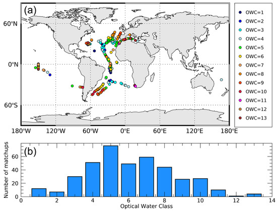
Figure 1.
Geographical distribution of the matchup dataset (N = 396) used for the analysis. Each datapoint is also associated with the specific Optical Water Class (OWC) (a). Number of matchups per OWC (b).
2.4. Statistical Assessment
Estimated satellite Cphyto () computed with Equation (3) was compared to reference in situ data () by computing the bias (δ; mg m−3), the relative bias in percentage (∇; in %), and the standard deviation of the difference (; mg m−3). The assessment was made for each OWC individually and for all matchups at once:
3. Results
Algorithm Performance for Cphyto Retrievals
Results and statistics of the comparison between satellite Cphyto estimates obtained with our algorithm and the previously published values, and in situ Cphyto, are reported in Table 1 and Figure 2. Overall, algorithms perform with ∇ values spanning from 23.7% to 203%. The algorithm here developed shows the smallest bias (∇ of 23.7%). By comparison, the algorithms based on a constant value have lower performance, and Gra15, Beh05, and MV17 showed a systematic overestimation for low Cphyto values (Table 1 and Figure 2).

Table 1.
Basic statistics for each single approach. For each approach is reported the bias (δ; in mg m−3), the standard deviation (; in mg m−3), and the relative percentage bias (∇; in %). Note that OWCs 1 and 2 are grouped in a single class to increase the number of observations available for the statistics. This is also replicated for OWCs 11, 12, and 13. The statistics using log10 transformed data for all OWCs are reported in Table S1.
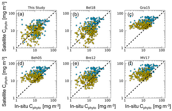
Figure 2.
Matchups between satellite Cphyto versus in situ Cphyto data for each algorithm (N = 396). The dashed line represents the 1:1 ratio. Gold dots represent in situ Cphyto data corresponding to OWCs 1–6; blue dots represent in situ Cphyto data for OWCs 7–13. Statistics are reported in Table 1.
The bbp-based algorithms that use a single constant value (Beh05, Bre12, and Bel18) show similar . Specifically, Bre12 has a value that is twice as high as that used in Beh05, and Bel18 has a value nearly three times larger than that of Beh05. ∇ ranges from 23.7% (Bel18) and 80.1% (Bre12), to 130.3% (Beh05), resulting in different performance in relation to the selection of the single value.
In the case of Beh05, a source of discrepancy leading to such a bias may be linked to the bbp input from the algorithm as also highlighted in [27]. Indeed, the original equation was derived using the GSM algorithm [29] for obtaining a relationship between Chl and bbp and thus for the estimation, instead of the QAA, applied here. In addition, it has recently been found that Raman scattering (here corrected prior to the QAA application) plays a fundamental role for the retrievals of bbp in very clear waters because, if not corrected, it results in overestimation of bbp [36,43].
However, these results highlight how the use of a single determines a strong overestimation of satellite Cphyto, in line with the results of MV17 (Table 1 and Figure 2). The comparison between our approach and previously published models underlines the necessity to account for the spatio-temporal variability of the for satellite-based Cphyto calculation. However, because Bre12 and Bel18 show relatively low bias, such approaches might be used alternatively to the new approach proposed here because it may occur in the most oligotrophic waters (e.g., subtropical gyre areas). Note that in Bre12, the was at 470 nm so that the overestimation of Cphyto can decrease if the is reported to the band of 443 nm.
The empirical algorithms of Gra15 and MV17 yield the worst results in terms of ∇. In the case of Gra15, this is the consequence of the few in situ measurements used for the algorithm definition, located in the Equatorial Pacific Ocean and in the Atlantic Ocean. Extrapolation of their algorithm, developed at 470 nm, to 443 nm, may also have had an effect. Regarding MV17, the results found are consistent with those reported in Tables 3 and 5 of their work.
MV17 reported that the geographical distribution of the in situ data, the median Cphyto concentrations, and the carbon-to-chlorophyll ratios are in agreement with previous observations in oligotrophic oceanic conditions [16,18]. The fact that the in situ Cphyto dataset used here contains only data from the picophytoplankton population must be taken into account for the interpretation of the algorithm evaluation. In most oligotrophic waters (OWCs from 1 to 6), δ shows the lowest values for all of the algorithms, with a maximum value of 14.4 mg m−3 (Table 1). However, when analyzing the ∇ index, the Cphyto computed by considering the spatio-temporal variability of is the most efficient (Table 1), with the exception of OWCs 5 and 6, for which Bel18 shows the best performance. Indeed, within OWCs in which picophytoplankton is expected to dominate (OWCs from 1 to 6), the performance of the majority of the tested algorithms generally improves (Table 1), with the exceptions of Gra15 and MV17. As expected, there is a decrease in the accuracy for all of the algorithms in the OWCs from 7 to 13. This could be influenced by the dominance of nano- and micro-phytoplankton (cell size > 2 μm) in these waters, whereas the picophytoplankton contribute in low relative proportions [14]. Because most of the bbp signal is due to particles with equivalent diameters larger than that those associated with picophytoplankton [23], a decreasing performance of the bbp-based algorithms in water dominated by larger cells (e.g., nano- and micro-phytoplankton) was expected (Table 1).
4. Discussion
4.1. Spatial and Temporal Distribution of Cphyto
The global mean climatology of Cphyto (Figure 3a) agrees with the expected geographical distribution [14]. Cphyto highs are found in the most productive regions such as the high latitude regions and coastal areas, and in upwelling systems such as those off Mauritania and Perù, the Benguela and Kuroshio currents, and along the equatorial belt of the Pacific Ocean (Figure 3a). Cphyto lows are found in mid-latitude areas such as the subtropical gyres or the Eastern Mediterranean Sea and Black Sea. Cphyto varies within the same order of magnitude of recent estimates made using satellite data [14] and biogeochemical models [44]. The two main oceanic regimes as defined by [45] are also highlighted from our analysis: “photoacclimation-dominance” and “biomass-dominance”. The former is typical of oligotrophic areas (e.g., subtropical gyres) where the variability of Chl is uncoupled from biomass and the process of acclimation to light and nutrients drives Chl variations [45]. In these areas, Cphyto shows the lowest mean values (<10 mg C m−3). Conversely, the latter is typical of most productive areas where Chl and bbp strongly covary [31,46]. The high Chl-bbp co-variability indicates that particles (and biomass) co-vary with phytoplankton abundance, whereas the physiological photoacclimation process plays a secondary role in determining the Chl variations; e.g., in the North Atlantic and Southern Oceans, Cphyto shows the highest mean values (>30 mg C m−3).
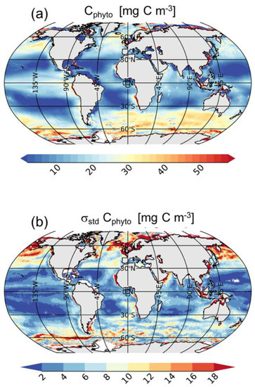
Figure 3.
Annual global mean (a) and standard deviation (b) of Cphyto. Note that at high latitudes the number of satellite observations used for the mean and standard deviation computations are lower than those used at low or mid-latitudes due to the winter darkness (i.e., high sun zenith angle).
The amplitude of seasonal variations (i.e., interannual variability) of Cphyto is shown in Figure 3b. Most of the variability is observed at high latitudes (e.g., Baltic Sea, Irish Sea, Norwegian Sea, North Sea), in the North Pacific and North Atlantic Oceans, and in the Southern Ocean, because σstd values are higher than 12 mg m−3. The North Atlantic and Southern Oceans are characterized by high seasonal variations due to intense productive months followed by unproductive periods [47,48,49] (Figures S2–S13). In the North Atlantic Ocean, Cphyto starts to increase in May, reaching the maximum values in June and July (>50 mg C m−3) following the spring bloom. Then, Cphyto decreases to the lowest values for the remainder of the year [47]. In the Southern Ocean, Cphyto follows the typical seasonal cycle with high values during the most productive months which occur from November to March (>50 mg C m−3). Highs are mostly observed in the Antarctic Circumpolar Current (ACC) and the Patagonia Shelf. Later, there is a decrease in Cphyto from May to September (Figures S2–S13). Additionally, the northwestern Indian Ocean, known to be an Oxygen Minimum Zone, as well as the Benguela upwelling system, also show significant variability in Cphyto, with σstd greater than 12 mg m−3. Conversely, mid-latitude areas (e.g., in the subtropical gyres), display much lower variability, with σstd less than 2 mg C m−3.
Figure S14 clearly shows how the single of Beh05 is located at the lowest limit of possible values, confirming that reported in [28], whereas the Bel18 and Bre12 single values are representative of a wider area. In the subtropical gyres, does not significantly deviate from the coefficient found by Beh05, but in the most productive regions (e.g., North Atlantic and Southern Oceans, high latitude seas, and coastal upwelling regions), they largely differ with great impact on Cphyto estimations. This discrepancy in Cphyto is still valid in the case of the use of Bel18 and Bre12 single values, but for other areas (e.g., in the subtropical gyres or in the Mediterranean Sea), the use of the single value of Bel18 or Bre12 yields an underestimation of Cphyto, whereas in the productive Arctic and Southern Oceans Cphyto is generally overestimated. This is also indicated in the seasonal variation as reported in the Figures S2–S13. In the North Atlantic Ocean, shows high values during the spring bloom and low values from December to April. However, in this area, the is only a small fraction of the entire bbp signal as the consequence of the high variability in the bbp and phytoplankton abundance [25,27] thus following the phytoplankton dynamics. In the Southern Ocean, and especially the region influenced by the ACC and Patagonia Shelf, shows highs from December to April (i.e., due to coccoliths) and lows in the period May–September in accordance also with the Cphyto seasonal cycle [25]. In less productive seas, the seasonal cycle of is smooth, suggesting low NAP variations. In these areas, the seasonal change is weak throughout the year but also dominates the bbp signal [25]. These areas are characterized by limited nutrient availability determining low Cphyto, mostly of picophytoplankton class, high bacterial, and detrital concentrations [50,51,52]. It follows that the use of a varying enables accounting for its seasonal variations in the Cphyto computation, giving the model more flexibility in relation to the change of the biogeochemical and trophic conditions.
4.2. Caveats of the Cphyto Algorithm
Three main caveats of the algorithm should be noted. The first is that Cphyto assumes a constant scaling factor, SF, equal to 13,000 mg C m−2, following [7]. This can be an additional possible source of error in the satellite retrievals of Cphyto. Therefore, one important future effort should be to investigate a refined scaling factor relating bbp to Cphyto coupled with the space–time variability as presented in this work. With this perspective, additional laboratory work should be done to evaluate if change in SF values can affect the Cphyto estimations.
The second caveat of the algorithm is that it relies on a tight relationship between bbp and Chl, which is influenced by the algorithms (including the atmospheric correction) used for Chl and bbp retrievals, in addition to the environmental conditions. In some areas of the subtropical gyres, the Chl–bbp relationship showed S < 0.95 (Figures S2–S13) and r smaller than or close to 0, as also reported by [28]. The main reason for this relationship may be the photoacclimation process, known to be dominant in such areas over the year, and which introduces variability in Chl that is unrelated to biomass. In these areas, our refined method must be applied with caution. With this perspective, one future challenge is to solve this limitation in computation and, consequently, in the satellite Cphyto. Indeed, as the subtropical gyres cover about 60% of the global ocean, it can be of a great importance to compute Cphyto and Chl:Cphyto to understand oceanic biogeochemical cycles. Conversely, the remaining areas of global ocean (e.g., the North Atlantic Ocean) present significant positive r and highly significant S (Figures S2–S13) throughout the year, indicating that either bbp or Chl can be used for determining the phytoplankton dynamics and distribution, as expected in open-ocean waters [27]. In these areas, the algorithm performance is robust.
The third caveat is that the algorithm validation is restricted only to in situ Cphyto data associated with picophytoplankton carbon. It determines that the algorithm performance has to be interpreted with caution in those areas where other phytoplankton size classes dominate. This means that, currently, it is not possible to define the accuracy for OWCs from 7 to 13. Indeed, Table 1 shows that there is a decrease in the accuracy for all of the algorithms in the OWCs where nano- and micro-phytoplankton dominates. Thus, one future need is to improve the in situ Cphyto dataset with new measurements representative of all of the phytoplankton size classes.
5. Conclusions and Future Perspectives
In this work, a revisited version of the original bbp-based algorithm for Cphyto retrieval from space [7] was proposed. The spatio-temporal variations of the background backscattering coefficient of non-algal particles () is the crucial part of this refinement, and builds upon a series of recent studies [25,27,28]. The main findings are:
However, we acknowledge that the refined algorithm presented here could be improved by addressing the caveats mentioned above. Enlarging the databases of quality-controlled and freely accessible in situ Cphyto at the different size-classes (pico-, nano-, and micro-), measured simultaneously with an array of optical variables (particularly bbp) could help to reduce uncertainties in Cphyto retrieval from space. Improving the accuracy of satellite Cphyto could be of great importance to adding new knowledge regarding the contribution of phytoplankton to particulate organic carbon, and for the validation of ocean primary productivity and biogeochemical models at a wider scale [8,12].
Supplementary Materials
The following are available online at https://www.mdpi.com/2072-4292/12/21/3640/s1, Figure S1: Scheme of the algorithm developed, Table S1: Basic statistics of the validation analysis for all the matchup with log10 transformed data: Figures S2–S13: global monthly climatologies of (a), 1-σ uncertainty (b), significance S (c) and Cphyto (d); Figure S14: global mean and standard deviation maps.
Author Contributions
Conceptualization, M.B., J.P., V.M.-V. and S.M.; Methodology, M.B., J.P., E.O. and S.M.; Data curation, M.B., S.M., J.P.; Writing—review and editing, all authors contributed equally. All authors have read and agreed to the published version of the manuscript.
Funding
M. Bellacicco has a postdoctoral fellowship by the European Space Agency (ESA). This work was supported by the ESA Living Planet Fellowship Project PHYSIOGLOB: Assessing the inter-annual physiological response of phytoplankton to global warming using long-term satellite observations, 2018–2020. Jaime Pitarch is supported by the Copernicus Climate Change Service contract: Independent Assessment of ECVs (C3S_511).
Acknowledgments
We thank ESA OC-CCI for providing publicly available ocean colour data (https://esa-oceancolour-cci.org). Giorgio Dall’Olmo (PML), Rosalia Santoleri (CNR-ISMAR), Vittorio Brando (CNR-ISMAR) and Marie-Hélène Rio (ESA) are thanked for all the inputs, suggestions and discussion done since the early version of the manuscript. We wish to thank the four anonymous reviewers for their criticisms and suggestions that helped the manuscript to be improved.
Conflicts of Interest
The authors declare no conflict of interest.
References
- Siegel, D.A.; Buesseler, K.O.; Doney, S.C.; Sailley, S.F.; Behrenfeld, M.J.; Boyd, P.W. Global assessment of ocean carbon export by combining satellite observations and food-web models. Glob. Biogeochem. Cycles 2014, 28, 181–196. [Google Scholar] [CrossRef]
- Boyce, D.G.; Lewis, M.R.; Worm, B. Global phytoplankton decline over the past century. Nature 2010, 466, 591–596. [Google Scholar] [CrossRef] [PubMed]
- Dutkiewicz, S.; Hickman, A.E.; Jahn, O.; Henson, S.; Beaulieu, C.; Monier, E. Ocean colour signature of climate change. Nat. Commun. 2019, 10, 578. [Google Scholar] [CrossRef] [PubMed]
- O’Reilly, J.E.; Werdell, P.J. Chlorophyll algorithms for ocean color sensors—OC4, OC5 & OC6. Remote Sens. Environ. 2019, 229, 32–47. [Google Scholar] [CrossRef]
- Laws, E.A.; Bannister, T.T. Nutrient- and light-limited growth of Thalassiosira fluviatilis in continuous culture, with implications for phytoplankton growth in the ocean1. Limnol. Oceanogr. 1980, 25, 457–473. [Google Scholar] [CrossRef]
- Behrenfeld, M.J.; Boss, E.S. Resurrecting the Ecological Underpinnings of Ocean Plankton Blooms. Annu. Rev. Mar. Sci. 2014, 6, 167–194. [Google Scholar] [CrossRef] [PubMed]
- Behrenfeld, M.J.; Boss, E.; Siegel, D.A.; Shea, D.M. Carbon-based ocean productivity and phytoplankton physiology from space. Glob. Biogeochem. Cycles 2005, 19. [Google Scholar] [CrossRef]
- Westberry, T.; Behrenfeld, M.J.; Siegel, D.A.; Boss, E. Carbon-based primary productivity modeling with vertically resolved photoacclimation. Glob. Biogeochem. Cycles 2008, 22. [Google Scholar] [CrossRef]
- Behrenfeld, M.J.; Halsey, K.H.; Milligan, A.J. Evolved physiological responses of phytoplankton to their integrated growth environment. Philos. Trans. R. Soc. B Biol. Sci. 2008, 363, 2687–2703. [Google Scholar] [CrossRef] [PubMed]
- Zhai, L.; Platt, T.; Tang, C.; Dowd, M.; Sathyendranath, S.; Forget, M.-H. Estimation of phytoplankton loss rate by remote sensing. Geophys. Res. Lett. 2008, 35. [Google Scholar] [CrossRef]
- Zhai, L.; Platt, T.; Tang, C.; Sathyendranath, S.; Fuentes-Yaco, C.; Devred, E.; Wu, Y. Seasonal and geographic variations in phytoplankton losses from the mixed layer on the Northwest Atlantic Shelf. J. Mar. Syst. 2010, 80, 36–46. [Google Scholar] [CrossRef]
- Dutkiewicz, S.; Hickman, A.E.; Jahn, O.; Gregg, W.W.; Mouw, C.B.; Follows, M.J. Capturing optically important constituents and properties in a marine biogeochemical and ecosystem model. Biogeosciences 2015, 12, 4447–4481. [Google Scholar] [CrossRef]
- Fossum, K.N.; Ovadnevaite, J.; Ceburnis, D.; Dall’Osto, M.; Marullo, S.; Bellacicco, M.; Simó, R.; Liu, D.; Flynn, M.; Zuend, A.; et al. Summertime Primary and Secondary Contributions to Southern Ocean Cloud Condensation Nuclei. Sci. Rep. 2018, 8, 13844. [Google Scholar] [CrossRef]
- Martínez-Vicente, V.; Evers-King, H.; Roy, S.; Kostadinov, T.S.; Tarran, G.A.; Graff, J.R.; Brewin, R.J.W.; Dall’Olmo, G.; Jackson, T.; Hickman, A.E.; et al. Intercomparison of Ocean Color Algorithms for Picophytoplankton Carbon in the Ocean. Front. Mar. Sci. 2017, 4. [Google Scholar] [CrossRef]
- Martínez-Vicente, V.; Dall’Olmo, G.; Tarran, G.; Boss, E.; Sathyendranath, S. Optical backscattering is correlated with phytoplankton carbon across the Atlantic Ocean. Geophys. Res. Lett. 2013, 40, 1154–1158. [Google Scholar] [CrossRef]
- Graff, J.R.; Westberry, T.K.; Milligan, A.J.; Brown, M.B.; Dall’Olmo, G.; Dongen-Vogels, V.V.; Reifel, K.M.; Behrenfeld, M.J. Analytical phytoplankton carbon measurements spanning diverse ecosystems. Deep Sea Res. Part I Oceanogr. Res. Pap. 2015, 102, 16–25. [Google Scholar] [CrossRef]
- Sathyendranath, S.; Stuart, V.; Nair, A.; Oka, K.; Nakane, T.; Bouman, H.; Forget, M.H.; Maass, H.; Platt, T. Carbon-to-chlorophyll ratio and growth rate of phytoplankton in the sea. Mar. Ecol. Prog. Ser. 2009, 383, 73–84. [Google Scholar] [CrossRef]
- Marañón, E.; Cermeño, P.; Huete-Ortega, M.; López-Sandoval, D.C.; Mouriño-Carballido, B.; Rodríguez-Ramos, T. Resource Supply Overrides Temperature as a Controlling Factor of Marine Phytoplankton Growth. PLoS ONE 2014, 9, e99312. [Google Scholar] [CrossRef]
- Kostadinov, T.S.; Siegel, D.A.; Maritorena, S. Retrieval of the particle size distribution from satellite ocean color observations. J. Geophys. Res. Ocean. 2009, 114. [Google Scholar] [CrossRef]
- Kostadinov, T.S.; Milutinović, S.; Marinov, I.; Cabré, A. Carbon-based phytoplankton size classes retrieved via ocean color estimates of the particle size distribution. Ocean Sci. 2016, 12, 561–575. [Google Scholar] [CrossRef]
- Roy, S.; Sathyendranath, S.; Platt, T. Size-partitioned phytoplankton carbon and carbon-to-chlorophyll ratio from ocean colour by an absorption-based bio-optical algorithm. Remote Sens. Environ. 2017, 194, 177–189. [Google Scholar] [CrossRef]
- Stramski, D.; Boss, E.; Bogucki, D.; Voss, K.J. The role of seawater constituents in light backscattering in the ocean. Prog. Oceanogr. 2004, 61, 27–56. [Google Scholar] [CrossRef]
- Organelli, E.; Dall’Olmo, G.; Brewin, R.J.W.; Tarran, G.A.; Boss, E.; Bricaud, A. The open-ocean missing backscattering is in the structural complexity of particles. Nat. Commun. 2018, 9, 5439. [Google Scholar] [CrossRef] [PubMed]
- Zhang, X.; Hu, L.; Xiong, Y.; Huot, Y.; Gray, D. Experimental Estimates of Optical Backscattering Associated with Submicron Particles in Clear Oceanic Waters. Geophys. Res. Lett. 2020, 47, e2020GL087100. [Google Scholar] [CrossRef]
- Bellacicco, M.; Cornec, M.; Organelli, E.; Brewin, R.J.W.; Neukermans, G.; Volpe, G.; Barbieux, M.; Poteau, A.; Schmechtig, C.; D’Ortenzio, F.; et al. Global Variability of Optical Backscattering by Non-algal particles From a Biogeochemical-Argo Data Set. Geophys. Res. Lett. 2019, 46, 9767–9776. [Google Scholar] [CrossRef]
- Brewin, R.J.W.; Dall’Olmo, G.; Sathyendranath, S.; Hardman-Mountford, N.J. Particle backscattering as a function of chlorophyll and phytoplankton size structure in the open-ocean. Opt. Express 2012, 20, 17632–17652. [Google Scholar] [CrossRef]
- Bellacicco, M.; Volpe, G.; Colella, S.; Pitarch, J.; Santoleri, R. Influence of photoacclimation on the phytoplankton seasonal cycle in the Mediterranean Sea as seen by satellite. Remote Sens. Environ. 2016, 184, 595–604. [Google Scholar] [CrossRef]
- Bellacicco, M.; Volpe, G.; Briggs, N.; Brando, V.; Pitarch, J.; Landolfi, A.; Colella, S.; Marullo, S.; Santoleri, R. Global Distribution of Non-algal Particles from Ocean Color Data and Implications for Phytoplankton Biomass Detection. Geophys. Res. Lett. 2018, 45, 7672–7682. [Google Scholar] [CrossRef]
- Garver, S.A.; Siegel, D.A. Inherent optical property inversion of ocean color spectra and its biogeochemical interpretation: 1. Time series from the Sargasso Sea. J. Geophys. Res. Ocean. 1997, 102, 18607–18625. [Google Scholar] [CrossRef]
- Dall’Olmo, G.; Westberry, T.K.; Behrenfeld, M.J.; Boss, E.; Slade, W.H. Significant contribution of large particles to optical backscattering in the open ocean. Biogeosciences 2009, 6, 947–967. [Google Scholar] [CrossRef]
- Dall’Olmo, G.; Boss, E.; Behrenfeld, M.; Westberry, T. Particulate optical scattering coefficients along an Atlantic Meridional Transect. Opt. Express 2012, 20, 21532–21551. [Google Scholar] [CrossRef] [PubMed]
- Jackson, T.; Sathyendranath, S.; Mélin, F. An improved optical classification scheme for the Ocean Colour Essential Climate Variable and its applications. Remote Sens. Environ. 2017, 203, 152–161. [Google Scholar] [CrossRef]
- Jackson, T.; Chuprin, A.; Sathyendranath, S.; Grant, M.; Zühlke, M.; Dingle, J.; Storm, T.; Boettcher, M.; Fomferra, N. Ocean Colour Climate Change Initiative (OC_CCI)—Interim Phase. Product User Guide. D3.4 PUG. 2019. Available online: https://esa-oceancolour-cci.org/sites/esa-oceancolour-cci.org/alfresco.php?file=a68aa514-3668-4935-9235-fca10f7e8bee&name=OC-CCI-PUG-v4.1-v1.pdf (accessed on 22 December 2019).
- Lee, Z.; Carder, K.L.; Arnone, R.A. Deriving inherent optical properties from water color: A multiband quasi-analytical algorithm for optically deep waters. Appl. Opt. 2002, 41, 5755–5772. [Google Scholar] [CrossRef]
- Lee, Z. Update of the Quasi-Analytical Algorithm (QAA_v6). Available online: http://www.ioccg.org/groups/Software_OCA/QAA_v6_2014209.pdf (accessed on 22 December 2019).
- Pitarch, J.; Bellacicco, M.; Organelli, E.; Volpe, G.; Colella, S.; Vellucci, V.; Marullo, S. Retrieval of Particulate Backscattering Using Field and Satellite Radiometry: Assessment of the QAA Algorithm. Remote Sens. 2020, 12, 77. [Google Scholar] [CrossRef]
- Brewin, R.J.W.; Sathyendranath, S.; Müller, D.; Brockmann, C.; Deschamps, P.-Y.; Devred, E.; Doerffer, R.; Fomferra, N.; Franz, B.; Grant, M.; et al. The Ocean Colour Climate Change Initiative: III. A round-robin comparison on in-water bio-optical algorithms. Remote Sens. Environ. 2015, 162, 271–294. [Google Scholar] [CrossRef]
- Mélin, F.; Berthon, J.-F.; Zibordi, G. Assessment of apparent and inherent optical properties derived from SeaWiFS with field data. Remote Sens. Environ. 2005, 97, 540–553. [Google Scholar] [CrossRef]
- Melin, F.; Zibordi, G.; Berthon, J. Uncertainties in Remote Sensing Reflectance from MODIS-Terra. IEEE Geosci. Remote Sens. Lett. 2012, 9, 432–436. [Google Scholar] [CrossRef]
- Sathyendranath, S.; Brewin, R.J.W.; Brockmann, C.; Brotas, V.; Calton, B.; Chuprin, A.; Cipollini, P.; Couto, A.B.; Dingle, J.; Doerffer, R.; et al. An Ocean-Colour Time Series for Use in Climate Studies: The Experience of the Ocean-Colour Climate Change Initiative (OC-CCI). Sensors 2019, 19, 4285. [Google Scholar] [CrossRef]
- Press, W.H.; Teukolsky, S.A.; Vetterling, W.T.; Flannery, B.P. Numerical Recipes in C; Cambridge University Press: Cambridge, UK, 1988. [Google Scholar]
- Resplandy, L.; Lévy, M.; McGillicuddy, D.J., Jr. Effects of Eddy-Driven Subduction on Ocean Biological Carbon Pump. Glob. Biogeochem. Cycles 2019, 33, 1071–1084. [Google Scholar] [CrossRef]
- Westberry, T.K.; Boss, E.; Lee, Z. Influence of Raman scattering on ocean color inversion models. Appl. Opt. 2013, 52, 5552–5561. [Google Scholar] [CrossRef]
- Arteaga, L.; Pahlow, M.; Oschlies, A. Modeled Chl:C ratio and derived estimates of phytoplankton carbon biomass and its contribution to total particulate organic carbon in the global surface ocean. Glob. Biogeochem. Cycles 2016, 30, 1791–1810. [Google Scholar] [CrossRef]
- Siegel, D.A.; Maritorena, S.; Nelson, N.B.; Behrenfeld, M.J. Independence and interdependencies among global ocean color properties: Reassessing the bio-optical assumption. J. Geophys. Res. Ocean. 2005, 110. [Google Scholar] [CrossRef]
- Westberry, T.K.; Dall’Olmo, G.; Boss, E.; Behrenfeld, M.J.; Moutin, T. Coherence of particulate beam attenuation and backscattering coefficients in diverse open ocean environments. Opt. Express 2010, 18, 15419–15425. [Google Scholar] [CrossRef]
- Westberry, T.K.; Schultz, P.; Behrenfeld, M.J.; Dunne, J.P.; Hiscock, M.R.; Maritorena, S.; Sarmiento, J.L.; Siegel, D.A. Annual cycles of phytoplankton biomass in the subarctic Atlantic and Pacific Ocean. Glob. Biogeochem. Cycles 2016, 30, 175–190. [Google Scholar] [CrossRef]
- Balch, W.M. The Ecology, Biogeochemistry, and Optical Properties of Coccolithophores. Annu. Rev. Mar. Sci. 2018, 10, 71–98. [Google Scholar] [CrossRef]
- Barbieux, M.; Uitz, J.; Bricaud, A.; Organelli, E.; Poteau, A.; Schmechtig, C.; Gentili, B.; Obolensky, G.; Leymarie, E.; Penkerc’h, C.; et al. Assessing the Variability in the Relationship between the Particulate Backscattering Coefficient and the Chlorophyll a Concentration from a Global Biogeochemical-Argo Database. J. Geophys. Res. Ocean. 2018, 123, 1229–1250. [Google Scholar] [CrossRef]
- Heywood, J.L.; Zubkov, M.V.; Tarran, G.A.; Fuchs, B.M.; Holligan, P.M. Prokaryoplankton standing stocks in oligotrophic gyre and equatorial provinces of the Atlantic Ocean: Evaluation of inter-annual variability. Deep Sea Res. Part II: Top. Stud. Oceanogr. 2006, 53, 1530–1547. [Google Scholar] [CrossRef]
- Grob, C.; Ulloa, O.; Claustre, H.; Huot, Y.; Alarcon, G.; Marie, D. Contribution of picoplankton to the total particulate organic carbon concentration in the eastern South Pacific. Biogeosciences 2007, 4, 837–852. [Google Scholar] [CrossRef]
- Organelli, E.; Dall’Olmo, G.; Brewin, R.J.; Nencioli, F.; Tarran, G.A. Drivers of spectral optical scattering by particles in the upper 500 m of the Atlantic Ocean. Opt. Express 2020, 28, 34147–34166. [Google Scholar] [CrossRef]


Publisher’s Note: MDPI stays neutral with regard to jurisdictional claims in published maps and institutional affiliations. |
© 2020 by the authors. Licensee MDPI, Basel, Switzerland. This article is an open access article distributed under the terms and conditions of the Creative Commons Attribution (CC BY) license (http://creativecommons.org/licenses/by/4.0/).