Abstract
The residual ionospheric error (RIE) from higher-order terms in the refractive index is not negligible when using global navigation satellite system (GNSS) radio occultation (RO) data for climate and meteorology applications in the stratosphere. In this study, a new higher-order bending angle RIE correction named “Bi-local correction approach” has been implemented and evaluated, which accounts for the ray path splitting of the dual-frequency GNSS signals, the altitude of the low Earth orbit (LEO) satellite, the ionospheric inbound (GNSS to tangent point) vs. outbound (tangent point to LEO) asymmetry, and the geomagnetic field. Statistical results based on test-day ensembles of RO events show that, over the upper stratosphere and mesosphere, the order of magnitude of the mean total RIE in the bi-local correction approach is 0.01 μrad. Related to this, the so-called electron-density-squared (Ne2) and geomagnetic (BNe) terms appear to be dominant and comparable in magnitude. The BNe term takes negative or positive values, depending on the angle between the geomagnetic field vector and the direction of RO ray paths, while the Ne2 term is generally negative. We evaluated the new approach against the existing “Kappa approach” and the standard linear dual-frequency correction of bending angles and found it to perform well and in many average conditions similar to the simpler Kappa approach. On top of this, the bi-local approach can provide added value for RO missions with low LEO altitudes and for regional-scale applications, where its capacity to account for the ionospheric inbound-outbound asymmetry as well as for the geomagnetic term plays out.
1. Introduction
Global navigation satellite system (GNSS) radio occultation (RO) [1,2] is an innovative atmospheric remote sensing technique, which can deliver global coverage, all-weather capability, long-term stability, traceability to the international standard (SI) of time, high vertical resolution and high accuracy of atmospheric profile retrievals (bending angle, refractivity, pressure, temperature, humidity profiles). It has been demonstrated that GNSS RO data play an important role in both decadal-scale climate change analysis [3,4,5,6] and numerical weather prediction (NWP) [5,7,8,9] applications, particularly in the upper troposphere and lower stratosphere altitude region.
Nevertheless, the ionosphere is one of the significant error sources of the GNSS RO technique, and a standard dual-frequency linear combination of RO bending angles is usually applied to correct the first order ionospheric effect [10,11,12]. However, the higher-order residual ionospheric errors (RIEs) after this correction are still not negligible for high-accuracy applications such as global climate change analysis and NWP [3,13,14,15]. This applies especially above about 35 km altitude, i.e., from the upper stratosphere upwards, where the RIEs become increasingly relevant compared to the exponentially decreasing magnitude of the neutral atmospheric bending angle [14,16,17,18]. Therefore, it is important to better understand and further mitigate the RIEs for enabling benchmark-quality stratospheric RO retrievals.
The RIEs’ characteristics and impact on the RO atmospheric profile retrievals have been investigated thoroughly [10,11,13,16,17,18,19,20,21,22,23,24], and several approaches of higher-order correction in GNSS RO bending angles have been developed so far [16,17,21,25].
Initially, the standard correction approach using a dual-frequency linear combination of bending angles was proposed by Vorob’ev and Krasil’nikova in 1994 [10], these authors also conducted an estimation of the residual errors of this approach, which indicated that the residual errors increased as a function of the electron density-squared over the vertical profile [10]. Recently, building on these early works, the so-called “Kappa correction approach” for mitigating the higher order RIEs was proposed and tested by using a simple one-dimensional ionospheric model [17], which adds a fairly simple higher-order squared-bending-angle difference term to the standard correction. Subsequently, the Kappa approach was validated and evaluated in more detailed simulations with a complex three-dimensional ionospheric model [18]. Meanwhile it is also applied in operational processing of the RO data from the European Meteorological Operational satellites mission (MetOp-A/-B/-C). More recently, Angling et al. further improved the modeling of the “Kappa coefficient” in this formulation, by accounting for its dependencies on solar zenith angle, solar flux (F10.7 index), and altitude [25].
In recent years, a couple of studies have also assessed the characteristics of bending angle RIEs with solar activity, with latitudinal region, and with or without the assumption of ionospheric spherical symmetry and of co-existing RO observing system errors, using end-to-end simulations for single RO events and a full-day ensemble of RO events [14,15]. A follow-up study also conducted a detailed along ray path analysis of atmospheric and ionospheric refractivity, impact parameter changes, accumulated bending angles and RIEs under asymmetric and symmetric ionospheric structures [26]. As shown in these explanatory simulation studies, in overall agreement with the empirical study of Danzer et al. [21], the RIE biases have a clear tendency to be negative and a bias magnitude increasing with solar activity as well as being affected by deviations from ionospheric spherical symmetry. Recently, the impact of the RIE correction by the “Kappa approach”, both with the original and improved Kappa coefficient modeling [17,25], was analyzed for multi-year radio occultation climatologies and RIE magnitude increases from about 0.2 to 2 K were found near 40 km altitude from low to high solar activity conditions [27].
The motivation of this paper is to investigate a new more refined bending angle RIE correction approach that was recently proposed by Syndergaard and Kirchengast [28]. The refinement involves a rigorous and more advanced derivation of higher-order terms taking into account the following factors: (1) the influence of ray path splitting of the dual-frequency GNSS signals, (2) the influence of the geomagnetic field in the ionospheric refractive index, (3) the influence of ionization differences along the occultation rays, i.e., asymmetries in electron content between inbound (from GNSS satellite to tangent point, TP) and outbound (from TP to low Earth orbit (LEO) satellite) ray path regions, and (4) the influence of the local electron density at the low Earth orbit (LEO) satellite.
The influence of horizontal variations across the ionosphere, breaking local spherical symmetry about the TP location, is difficult to handle analytically in a general way. The idea followed in [28], is therefore to assume that the horizontal electron density variations between inbound and outbound regions are confined to a limited transition region between the inbound and outbound ray path parts (effectively situated above the TP location), but otherwise along each of the inbound and outbound paths the horizontal variations are zero.
In this way, the impact parameter for ray paths entering the neutral atmosphere, i.e., for rays with TP altitude below the ionosphere (in practice those from 80 km downwards), is constant along the path, and the same for the inbound and outbound paths, although the electron density fields on each side are different. This is because the paths at the inbound and outbound side each experience a spherically symmetric ionosphere (assuming the neutral atmosphere in between is also spherically symmetric). Syndergaard and Kirchengast [28] refer to this hence as “Bi-local spherical symmetry” (Figure 1), also lending the name to the new correction approach, henceforth referred to as the “Bi-local correction approach”. Although these assumptions are still a significant simplification, they allowed the derivation of a more general analytical expression for the bending angle RIE correction than in previous works.
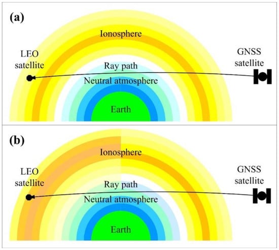
Figure 1.
Radio occultation geometry between global navigation satellite system (GNSS) transmitter and low Earth orbit (LEO) receiver satellites, schematically illustrating the signal ray path passing through the ionosphere and the atmosphere, as well as the overall local spherical symmetry assumption (a) in contrast to the bi-local spherical symmetry assumption (b).
In this study, we test and evaluate the new approach more thoroughly and hence implement it in a real RO processing setup, involving the use of a 3-dimensional ionospheric electron density model (Electron density (Ne) University of Graz model, NeUoG [29]), a geomagnetic field model (International Geomagnetic Reference Field, IGRF [30]), and of vertical total electron content (vTEC) maps from ground-based GNSS observations (provided operationally by the International GNSS Service, IGS [31], using the general IGS data product “igsg”).
The scientific questions are then how well the bi-local correction approach works under more realistic distributions of ionization than the ones assumed in the derivation [28], and how it compares to other existing approaches, in particular the recently introduced Kappa correction approach [17,18,25]. A key point of the study is assessment using real RO observation data from a diversity of RO missions with different LEO characteristics, namely the European MetOp-A/-B, the Gravity Recovery And Climate Experiment (GRACE) and the Challenging Mini-satellite Payload (CHAMP).
In Section 2, the existing ionospheric correction methods and in particular the new bi-local correction method are described algorithmically, the implementation of the bi-local approach in the reference occultation processing system (rOPS) is introduced, and the setup of the simulations for the performance evaluation is described. The evaluation results are presented in Section 3 and a detailed discussion and interpretation of these results is given in Section 4. The conclusions are provided in Section 5, where the strengths and limitations of the new approach are outlined.
2. Correction Approach and Implementation Setup
The Earth’s ionosphere is a mixed neutral-and-ionized gas consisting mainly of free electrons, ions, and neutral atoms and molecules, located at the altitude range of around 80 to 1000 km. Since the ionosphere is a dispersive medium, the magnitudes of GNSS signal carrier excess phase and bending angles are related to the carrier frequency. The signal propagation in the ionosphere is also affected by the geomagnetic field strength and direction. Following [32], for right-hand circularly polarized GNSS signals, the series expansion of the ionospheric refractive index can be accurately approximated by:
where the two constants and , is the electron density, B is the geomagnetic field strength, θ is the angle between the geomagnetic field vector and the ray propagation direction, is the GNSS signal frequency for Global Positioning System (GPS) signals, = 1.57542 GHz and = 1.22760 GHz), and the fundamental constants in C and K are elementary charge e, electron mass m, and permittivity of vacuum .
The standard approach to correcting the ionospheric effect is to use a dual-frequency linear combination of bending angles in GNSS RO data processing [10], expressed by:
where and are the two bending angles derived from the two GNSS frequency signals at the impact parameter α, and is the resulting linearly corrected bending angle that is corrected for the f−2 term of Equation (1) but has the other higher-order terms uncorrected, as well as a dominating error related to the ray path splitting, which is proportional to f−4 [16].
Healy and Culverwell [17] proposed a modification to this standard ionospheric correction that can be written in the following form:
where the first two terms on the right-hand side comprise the standard linear correction formulated as a correction term subtracted from , and is an additional higher-order RIE correction proportional to f−4, with these terms formulated as:
where is a slowly varying function of the impact parameter. In a follow-on study by Angling et al. [25], the RIE correction was analyzed for its dependency on various parameters using an ionospheric model, which led to a model-based “empirical” expression for the function :
where , , , are coefficients (with the values given in [25]; they are positive values so that is always positive and hence is always negative), is the solar flux index, is the solar zenith angle, and z is the altitude (for which the impact altitude can also be used, being essentially the same for the stratospheric and mesospheric altitudes of interest).
2.1. Formulation of Bi-Local RIE Model
The bi-local correction approach was proposed by Syndergaard and Kirchengast [28]. The key result Equation, the bi-local correction term, can be expressed in the form:
where is the total bi-local higher-order RIE correction term composed of (in order of appearance) a geomagnetic term, an electron density-squared term, and a local-LEO component term (the last term being only appreciable for non-circular orbits and large electron densities at the LEO). In Equation (7), is the geomagnetic field strength along the ray path (i.e., ), is the radius vector (magnitude) of the LEO satellite, is a geometric scaling variable determined by geometry parameters (see [28] for details), Ne(rL) is the local electron density at the LEO satellite, and other symbols are as defined previously. The functional is a ray path integral function from GNSS to LEO that can be described by inbound, outbound, and another local-LEO component as follows:
where X formally denotes either or , as contained in the respective terms of Equation (7). The relation between Equation (7) and Equation (5) was given in [28]. Basically, Equation (5) can be derived from the electron density-squared term in Equation (7), using simplified assumptions about the electron density, including local spherical symmetry and zero density at the LEO orbit and above. As a side note, it can be shown that, to the lowest order:
which can be used in the last term of Equation (7) or in Equation (5) to obtain purely modelled RIE results free of observational errors. As a baseline, though, we have used the observed bending angles that are readily available as part of the profile retrievals.
The full correction equation is of identical form as for the Kappa correction method, Equation (3), just with the Kappa correction term replaced by the bi-local correction:
2.2. Processing Setup for the Bi-Local Correction in the rOPS
2.2.1. rOPS as the System for RIE Correction Evaluation
The rOPS is a reference occultation processing system [33,34], developed at the Wegener Center for Climate and Global Change (WEGC) at the University of Graz, Austria, that aims to realize the benchmark quality potential of RO by establishing (1) a reliable and accurate retrieval with residual relative numerical uncertainties below 10−4, and (2) integrating a complete uncertainty propagation chain from RO raw tracking data and high accuracy GNSS orbit data, and relevant side influences, through four processors to atmospheric profiles [35]. Figure 2 shows the main components of the rOPS as well as the main interactions, where the occultation data processing (ODP) subsystem is the core subsystem provided for the retrieval of the level one and level two profiles [36,37,38,39,40].
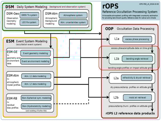
Figure 2.
Overview of the reference occultation processing system (rOPS) in the form of a functional block diagram, illustrating the logic of the system modeling and data analysis approach, indicating its main subsystems and the occultation data processing with the processors, highlighting the level 1b (L1b) data processor where the bi-local bending angle residual ionospheric error (RIE) correction is implemented with the red box.
Overall and for input to the ODP, the two major system modeling layers, background daily system modeling and occultation event system modeling, operate once per day, and once per event, respectively. They feed the different processors of the ODP subsystem and contain several subsystems to do so. The daily system modeling (DSM) consists of two subsystems, the DSM geometry (DSM-Geo) including the orbit modeling [41] and the DSM atmosphere (DSM-Atm).
The event system modeling (ESM) consists of three subsystems, the ESM for geometry and environment (ESM-GE), the ESM for atmosphere (ESM-Atm) and the ESM for residual bias modeling (ESM RB).
The bending angle ionospheric correction methods are embedded in the ODP subsystem at the level 1b processor [36,37,38], which is highlighted with a red box in Figure 2. Currently, the rOPS system uses the standard ionospheric correction, optionally improved by the Kappa correction, to mitigate the ionospheric effects. We have now additionally integrated the bi-local correction approach into the rOPS.
2.2.2. Implementation of the Bi-Local Correction Approach
The higher-order RIE correction in the rOPS has been augmented by integrating the bi-local method as a prototype processing capacity, by coupling it as an alternative option into the rOPS ODP level 1b (L1b) processor for bending angle retrieval. This integration is summarized below by making clear in detail the relevant inputs and outputs of the bi-local correction approach, before we dive into results in Section 3.
As evident from the correction term formulation in Section 2.1 above, the bi-local approach is a more complex and hence in principle a more capable analytical approach than the Kappa approach. Table 1, Table 2 and Table 3 summarize the fairly comprehensive input parameters and variables needed, and Table 4 collects all output variables of the bi-local correction available from the rOPS for the evaluations.

Table 1.
Basic inputs for the bi-local correction, from preparatory computations in the rOPS.
Table 2.
Derived inputs for the bi-local correction, from the Electron density (Ne) University of Graz model (NeUoG) and the International Geomagnetic Reference Field (IGRF)-12 model.
Table 3.
Input constants for the bi-local correction in the rOPS.
Table 4.
Outputs of the bi-local correction approach as integrated in the rOPS.
2.3. Setup of the Performance Evaluation Simulations
The solar, ionospheric and geomagnetic conditions are major space environment factors that affect the bending angle RIEs, and the ionospheric electron density and geomagnetic field intensity are therefore main input parameters of the bi-local correction approach.
In order to investigate their effects on the bending angle RIEs, in this section, the solar, ionospheric, and geomagnetic environment conditions of chosen test days will be described via solar activity F10.7 index, IGS vTEC maps, and geomagnetic field intensity maps. Along with this, the NeUoG ionospheric electron density model and the IGRF geomagnetic field model, also used in this study, will be briefly introduced.
2.3.1. Solar and Ionospheric Conditions
The solar radio flux at 10.7 cm (2800 MHz) is one of the longest running records of solar activity. reported in “solar flux units”, (s.f.u.), the F10.7 index can vary from near 50 s.f.u. to near 300 s.f.u., over the course of a solar cycle [31]. Figure 3a shows the time series of monthly mean F10.7 index from 2000 to 2018. According to the time series of monthly mean and daily mean F10.7 indices, as well as the available GNSS RO data sets, we selected July 2008 and May/July 2013 as low and high solar activity months, within which we (in essence arbitrarily) selected the 15 July 2008 as the low solar activity test day, and 15 May 2013 and 15 July 2013 as high solar activity test days, in our study.
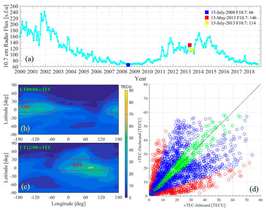
Figure 3.
Time series of monthly mean F10.7 index for the years from 2000 to 2018 (a) illustrating the three test days with square marks. The International GNSS Service (IGS) vTEC maps of the 00:00 UT (universal time) and 12:00 UT on 15 July 2013 are shown in panels (b,c), respectively. In panels (b,c), the equatorial day time (EDT) zone is highlighted with a red box. (d) vTEC scatter plot illustrating inbound vTEC (x-axis) vs. outbound vTEC (y-axis), classifying the ionospheric conditions into nearly symmetric (green; inbound-vs-outbound vTEC variation against mean vTEC within +/−10%), moderately asymmetric (blue; vTEC variation in between green and red), and strongly asymmetric (red; inbound-vs-outbound vTEC variation against mean vTEC larger than +/−50%).
Regarding the ionosphere, the NeUoG ionospheric model [29], which represents the 3D electron density distribution as a function of local time, season, and solar activity, was used in this study. It well represents realistic large-scale ionospheric variability but does not include small-scale ionospheric structures.
The ionospheric electron density (Ne) profiles used to implement the bi-local correction in this study are normalized Ne values by combining the NeUoG model electron density profiles and IGS vTEC maps. After the normalization, the Ne profiles have inherited the profile shapes of the NeUoG model electron density profiles and at the same time the vTEC value of the IGS vTEC maps (cf. Table 2). Using observation-based vTECs in this way, the model profiles are adjusted to be consistent with observed ionospheric conditions. Figure 3b,c show example IGS vTEC maps of 00:00 UT and 12:00 UT, respectively, on the test day 15 July 2013.
The ionospheric inbound and outbound vTEC conditions for the RO event locations are illustrated in Figure 3d, which shows the inbound vs. outbound vTEC of all RO events of the MetOp data (i.e., from all three test days, MetOp-A/-B missions). This illustration serves to support the understanding and interpretation of the subsequent results and discussion in Section 3 and Section 4.
2.3.2. Geomagnetic Conditions
The International Geomagnetic Reference Field (IGRF) comprises a series of mathematical models describing the large-scale internal part of the Earth’s magnetic field between epochs 1900 A.D. and the present. The 12th generation of the IGRF was adopted in December 2014. It updates the previous IGRF generation with a definitive main field model for epoch 2010.0, a main field model for epoch 2015.0, and a linear annual predictive secular variation model for 2015.0–2020.0 [30]. Figure 4 shows the main geomagnetic field components for the test day 15 July 2013.
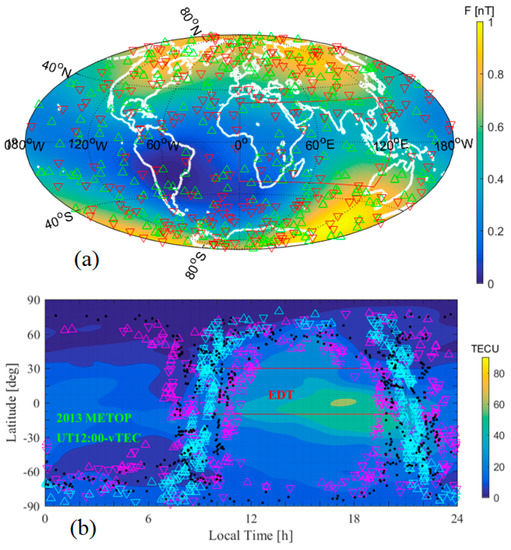
Figure 4.
Panel (a) shows the global distribution of mean tangent point locations of 493 European Meteorological Operational satellites mission (MetOp-B) RO events on 15 July 2013, including 255 RO events with negative geomagnetic (BNe) term (red downward-pointing triangles) and 238 RO events with positive BNe term (green upward-pointing triangles), the region highlighted with a red box includes 35 positive-BNe RO events but only 17 negative-BNe RO events. The background color map illustrates the mean geomagnetic field intensity for 15 July 2013. Panel (b) shows the local time (x-axis) vs. latitude (y-axis) distribution of the mean tangent points (black dots), inbound ion.mean-altitude points (magenta triangles), and outbound ion.mean-altitude points (cyan triangles) of 493 MetOp-B RO events on 15 July 2013. Similar to panel (a), the upward-pointing triangles denote positive BNe while downward-pointing triangles denote negative BNe. The background color map illustrates the IGS vTEC maps at 12:00 UT on 15 July 2013, and the equatorial day time (EDT) zone is highlighted with a red box.
Figure 4 also shows the global distribution of the mean tangent point locations of 493 MetOp-B RO events on 15 July 2013, including a globally comparable number of events with negative and positive geomagnetic (BNe) terms and highlighting a region with a significant excess of positive BNe events. The distribution of the MetOp-B RO events and their bending angle RIEs’ BNe term performance will be described and discussed in the following Section 3 and Section 4.
The ionospheric inbound and outbound vTEC conditions of the 493 MetOp-B RO events on 15 July 2013 are illustrated in Figure 4b, which shows the local time (x-axis) vs. latitude (y-axis) of the mean tangent points, inbound ion.mean-altitude points and outbound ion.mean-altitude points. This illustration serves to support the understanding and interpretation of the Figure 3d results and discussion in Section 3 and Section 4.
3. Results
3.1. Statistical Ensemble of Bending Angle RIE Profiles
In this subsection, the bending angle RIEs and their mean and standard deviation profiles of the bi-local and the Kappa correction approaches are shown and evaluated in different observing conditions. Firstly, the bi-local and Kappa bending angle RIE terms were interpolated to a standard vertical grid with 550 impact altitude levels (100 m spacing between levels) in the 25–80 km range, which are illustrated in Figure 5, Figure 6 and Figure 7. For obtaining the statistics, the ensemble mean and ensemble standard deviations were calculated level by level for any test ensemble of individual profiles.
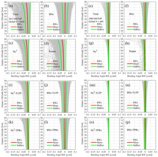
Figure 5.
Bi-local and Kappa bending angle RIE correction profiles and their statistics for the global ensemble high solar activity data set (left columns, MetOp-A/-B missions on 15 May and 15 July 2013) and low solar activity data set (right columns, MetOp-A mission on 15 July 2008). In the upper composite panels, the total bi-local bending angle correction (Total) and its BNe and electron-density-squared (Ne2) component terms, and the observed Kappa correction term are shown by subpanels (a–d) and (e–h). The lower composite panels show the inbound (TxTP) and outbound (TPRx) components of the Ne2 and BNe terms, in panels (i–l) and (m–p), respectively. In each subpanel, the individual bending angle RIEs (grey) and their mean (heavy red) and standard deviation (heavy green) are shown.
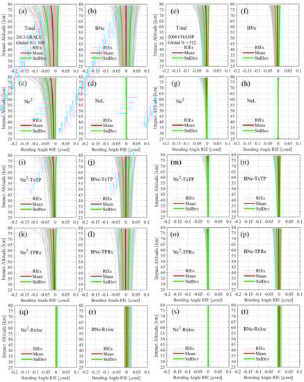
Figure 6.
Bi-local bending angle RIE correction profiles and their statistics for the global ensemble high solar activity data set (left columns, the Gravity Recovery And Climate Experiment (GRACE) mission on 15 May and 15 July 2013) and low solar activity data set (right columns, Challenging Mini-satellite Payload (CHAMP) mission on 14–16 July 2008). In the upper composite panels (top two rows), the total bi-local bending angle correction (Total) and its BNe, Ne2, and NeL component terms are shown by subpanels (a–d) and (e–h). The lower composite panels (third and fourth row) show the inbound (TxTP) and outbound (TPRx) components of the Ne2 and BNe terms, in panels (i–l) and (m–p), respectively. The bottom row panels show the Rx local (Rxloc) component of the Ne2 and BNe terms, in panels (q,r) and (s,t), respectively.
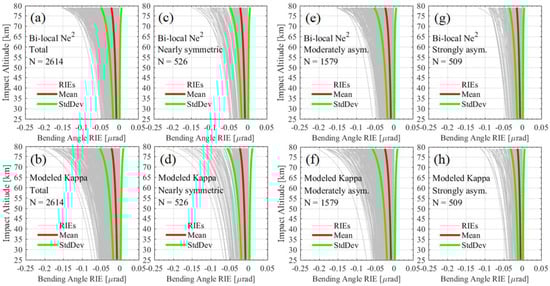
Figure 7.
Bi-local Ne2 term (top) and modeled Kappa (bottom) bending angle RIE correction profiles and their statistics, shown for the global ensemble total data set in (a,b) from the MetOp-A/-B RO events on all three test days as well as for the classified nearly symmetric, moderately asymmetric, and strongly asymmetric partial data sets in (c,d), (e,f), and (g,h), respectively.
As described by Equations (7) and (8), and in Table 4, the total bi-local bending angle RIE term has three components, i.e., BNe, electron-density-squared (Ne2), and NeL terms, wherein both the BNe and Ne2 terms have three subcomponents, i.e., inbound (TxTP), outbound (TPRx) and Rx local (Rxloc) terms. According to our study, for the MetOp-A/-B missions (Figure 5), at 60 km altitude and upwards, the order of magnitude of the mean total bi-local correction RIE is 0.01 μrad, and the BNe and Ne2 terms appear to be both significant terms with the same order of magnitude (see Figure 5).
As noted in Section 2.1, the NeL term is strongly related to the LEO satellite orbit altitude, orbit ellipticity and the in-situ ionospheric electron density. For the MetOp-A/-B missions, the magnitude of the NeL term is negligible (smaller than 0.001 μrad), while for the GRACE and CHAMP missions (Figure 6), it is smaller than 0.01 μrad even under high solar activity daytime conditions. Although in this way the NeL term of GRACE and CHAMP missions is substantially larger than that of the MetOp-A/-B missions, compared with the BNe and Ne2 terms it is still small and hence a minor term in practical application.
To specifically compare the performances of bending angle RIEs under low and high solar activity conditions, the MetOp-A dataset on 15 July 2008 and the MetOp-A/-B datasets on 15 May and 15 July 2013 were used, since these neatly correspond to low and high solar activity conditions, respectively. The results in Figure 5 indicate that all the bending angle RIE terms in the high solar activity test days are much larger than those in the low solar activity days in terms of the mean bias and standard deviation. Taking the bi-local total RIE and the Kappa correction terms as examples, one can see that from high solar activity days to low solar activity days at 75 km altitude level, the mean biases decreased from about −0.02 to −0.005 μrad, and the standard deviation decreased from about 0.03 to 0.01 μrad. Although Figure 6 shows the bending angle RIE terms of different missions (i.e., GRACE and CHAMP), the high solar activity vs. low solar activity behavior is similar.
To compare the performances of bi-local correction and Kappa correction approaches, Figure 5d,h subpanels show the observed Kappa correction result in order to show it side-by-side with the bi-local Ne2 correction term in Figure 5c,g. One can see that both the bi-local Ne2 term and the Kappa bending angle RIE have a clear negative tendency and similar magnitude values. The noisier behavior in Figure 5d,h is a result of using observed bending angles in the Kappa correction approach (Equation (5)), whereas the bi-local approach is based primarily on model estimations (except for using observed bending angles in the small last term of Equation (7)). Very large outliers of observed bending angle profiles were excluded according to quality control criteria, which led to bad-profile exclusion if one or more sampling points within the impact altitude range from 25 to 80 km showed values of that exceeded 0.1 μrad2. As a second step, the selected profiles were smoothed by a moving average filter with a window width of 10 km, before being used for Equation (5).
Inspecting Figure 5 and Figure 6 in more detail, we find further interesting aspects as follows. In Figure 5, for the MetOp-A/-B missions, comparing the (grey) profiles of the BNe and Ne2 terms, the BNe terms have negative and positive values, depending on the angle between the geomagnetic field vector and the ray path direction, while all the Ne2 terms are negative. The values of the Ne2 terms being systemically negative results in almost all the total bending angle RIE terms being negative as well. Comparing the statistics of the total bending angle RIE and Ne2 term, the average bias is similar, which means the effect of the BNe term on the global-mean climatology bending angle is small. This is because globally the BNe terms have almost the same amounts of positive-sign and negative-sign occurrences and hence cancel each other out when averaging over the RO events.
In Figure 6, similarly, for the GRACE and CHAMP missions, the BNe terms have negative and positive values, while all the Ne2 terms are negative. However, in the 2008 CHAMP mission ensemble data set, the average bias of the BNe term (Figure 6f) has a clear negative tendency, which causes the mean of the total bending angle RIE to be larger than that of the Ne2 terms alone. In both Figure 5 and Figure 6, comparing the profiles and statistics of the inbound Ne2 (Figure 5i,m and Figure 6i,m) and outbound Ne2 (Figure 5k,o and Figure 6k,o) terms, one can see that the inbound Ne2 terms are larger than those of the outbound. Whereas, comparing the profiles and statistics of the inbound BNe (Figure 5j,n and Figure 6j,n) and outbound BNe (Figure 5l,p and Figure 6l,p) terms, the inbound BNe terms are not always larger than those of the outbound. Specifically, the outbound BNe terms of the MetOp-A/-B missions (Figure 5l,p) are smaller than those of the inbound, while the outbound BNe terms of the GRACE (Figure 6l) and CHAMP (Figure 6p) missions are slightly larger than those of the inbound.
These different statistical behaviors of the GRACE and CHAMP mission data sets from those of MetOp-A/-B missions are most likely related to how their orbits were relative to the geomagnetic field and electron density environments on the test days. Therefore, a detailed analysis and explanation of the behavior of the Ne2 and BNe terms is given in the discussion in Section 4.
As shown in Equation (8), the order of magnitude of the Rxloc term is strongly related to the LEO satellite orbit altitude, the in-situ ionospheric electron density and geomagnetic field strength. For the MetOp-A/-B missions, the magnitude of the Rxloc term is negligible (smaller than 0.001 μrad). However, for the low orbit altitudes such as the GRACE and CHAMP missions (Figure 6q–t), the Rxloc BNe terms’ order of magnitude is up to 0.01 μrad, and reach a size near 0.025 μrad under high solar activity conditions, which therefore may cause slightly larger BNe terms, though they are smaller than the TxTP and TPRx terms.
To make a fair comparison between the bi-local Ne2 term and the Kappa bending angle RIE, we furthermore used Equation (9) to obtain modeled Kappa bending angle RIE correction profiles, based on the IGS vTEC maps and NeUoG ionospheric model. Results comparing these with the bi-local Ne2 term for different categories of ionospheric asymmetry are shown in Figure 7. One can see that the modeled Kappa bending angle RIEs are smoother than when using observed bending angles, and the total mean is similar to the total mean of the bi-local Ne2 terms, as shown in Figure 7a,b. However, in individual profiles, Kappa bending angle RIEs can be larger in size than those of the bi-local Ne2 terms. The reason for this is discussed in more detail below.
Looking at Figure 7 in more detail, the sizes of the mean of the Kappa bending angle RIEs and the bi-local Ne2 terms for the symmetric ensembles are larger than those of the asymmetric ensembles, because the nearly symmetrical RO events include those cases that have large vTEC at both inbound and outbound sides. For the nearly symmetric and moderately asymmetric ensembles, the sizes of the mean of the bi-local Ne2 terms are smaller than those of the Kappa bending angle RIEs, but in the strongly asymmetrical cases, it is the other way around.
To show these mean characteristics clearly in a single-panel intercomparison, Figure 8 illustrates the difference profiles of the mean bi-local Ne2 term and modeled Kappa bending angle RIEs (i.e., mean of bi-local Ne2 minus mean of modeled Kappa) for the three classified ensembles in Figure 7. Obviously, the difference profiles of the nearly symmetric and moderately asymmetric ensembles are positive, while the difference profile of the strongly asymmetrical ensemble is negative. This implies that the assumptions of the traditional spherical symmetry and the bi-local spherical symmetry, as shown in Figure 1, play key roles in causing the different behaviors.
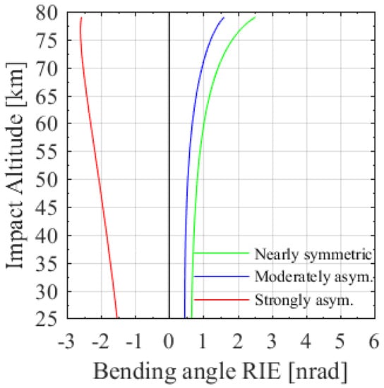
Figure 8.
Difference profiles of the mean bi-local Ne2 term and modeled Kappa bending angle RIEs (i.e., mean bi-local Ne2 minus mean modeled Kappa) for the classified nearly symmetric (green line), moderately asymmetric (blue line), and strongly asymmetric (red line) data sets, as illustrated in Figure 7.
In order to understand the reasons underlying the different behaviors of the bi-local Ne2 term and the modeled Kappa term bending angle RIEs, scatter plots of the Kappa factors and RIE terms are shown in Figure 9. Regarding the modeled and computed Kappa factors, the model-Kappa factor was calculated through Equation (6), using the , , , coefficients as given in [25], whereas the computed Kappa factor was calculated via , using for the bi-local Ne2 RIE term and computing by Equation (9). Note for the following discussion that, given the , the modeled Kappa RIE term was calculated by multiplying with the model-Kappa factor, whereas the bi-local Ne2 RIE term was obtained by instead multiplying the same with the computed Kappa factor.
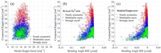
Figure 9.
Scatter plots of Kappa factor and bending angle RIE term values at 60 km impact altitude level illustrating the computed Kappa factor vs. the model-Kappa factor (according to [25]) in panel (a) as well as vs. the bi-local Ne2 term in panel (b) and vs. the modeled Kappa term in panel (c), respectively. Colors of the circles indicate the three classes of nearly symmetric (green), moderately asymmetric (blue), and strongly asymmetric (red) data sets (as illustrated in Figure 3d).
As shown in Figure 9a, for the nearly symmetric and moderately asymmetric ensembles, individually the computed Kappa values are compatible with the model-Kappa values (although there are differences related to the different ways the computed and model-Kappa values are calculated), while on average the computed Kappa values are a little smaller than the model-Kappa values. This is why the size of the mean of the bi-local Ne2 terms is smaller than that of the Kappa bending angle RIEs for those ensembles. However, for the strongly asymmetrical ensemble, both individually and on average, the computed Kappa values are systematically larger than the model-Kappa values. This is why the size of the mean of the bi-local Ne2 terms is larger than that of the Kappa bending angle RIEs for the strongly asymmetric ensemble.
In the strongly asymmetrical cases, individually the computed Kappa values are much larger than the model-Kappa values, but the most negative bi-local Ne2 terms are not numerically larger than the most negative Kappa bending angle RIEs in Figure 7. The reasons for this are, as shown in Figure 9b,c, that the largest computed Kappa values roughly correspond to the smallest RIEs, while the smallest computed Kappa values roughly correspond to the largest RIEs.
The differences in the computed Kappa and model-Kappa factor values reflect the differences between the two approaches used to calculate the Kappa values, including the fact that the computed Kappa values are based on the NeUoG model, whereas the model-Kappa values are derived/regressed based on the so-called NeQuick ionospheric model [25]. Additionally, because of the regression to obtain the , , , coefficients in [25], the model-Kappa values cannot be expected to give accurate bending angle RIEs for individual RO events even where is considered to be known (as in the theoretical calculation of RIEs here).
These results point to an added value of the bi-local correction approach compared to the Kappa approach, especially in strongly asymmetric cases, since the bi-local approach is theoretically accurate for the type of simplified cases of inbound/outbound ionospheric asymmetries as illustrated in Figure 1. However, it should also be kept in mind that this approach does not directly account for even more realistic asymmetries and that it might also give substantially deviating RIEs in such cases [28]. Furthermore, there is limitation from not knowing the “true” electron density distribution.
3.2. Statistical Results Inspected by Histograms
Figure 10 and Figure 11 show direct statistical comparisons of the bi-local BNe and Ne2 terms among the MetOp-A/-B, GRACE and CHAMP missions, by way of histograms. To also enable a regional cross-comparison in a challenging region, the data sets of equatorial day time zone (EDT) (latitude 10°S−30°N local time 9:00–21:00 h) are used in addition to the global dataset here. Based on the bi-local RIE data sets illustrated in Section 3.1, the BNe and Ne2 term averages over the 50–60 km impact altitude range were calculated profile by profile for the individual RO events, then the mean and median of these average BNe and Ne2 values were computed as well as the data counted into histogram bins.
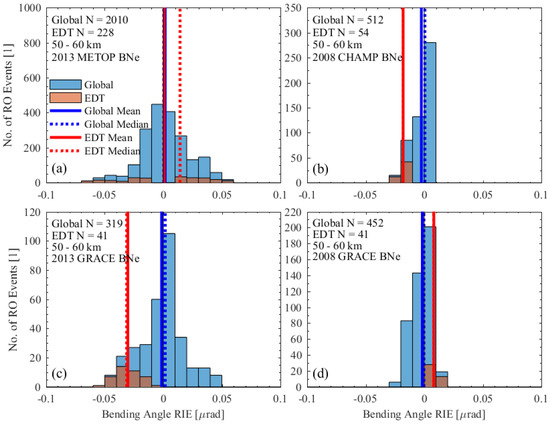
Figure 10.
Relationship between the histogram distribution of the number of RO events and the average value of the bi-local BNe term over 50–60 km impact altitude range for high solar activity data (left column, MetOp-A/-B (a) and GRACE (c) on 15 May and 15 July 2013) and low solar activity data (right column, CHAMP (b) and GRACE (d) on 14–16 July 2008). In each panel, the global (blue) and EDT (red) ensembles are presented as well as the global mean, global median, EDT mean, and EDT median as vertical lines in the corresponding colors (see legend in panel (a)).
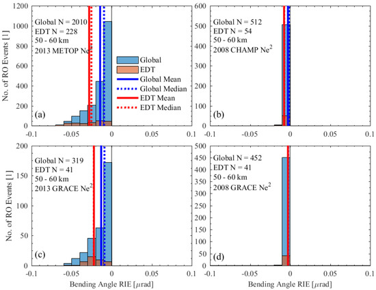
Figure 11.
Relationship between the histogram distribution of the number of RO events and the average value of the bi-local Ne2 term over 50–60 km impact altitude range for high solar activity data (left column, MetOp-A/-B (a) and GRACE (c) on 15 May and 15 July 2013) and low solar activity data (right column, CHAMP (b) and GRACE (d) on 14–16 July 2008). In each panel, the global (blue) and EDT (red) ensembles are presented as well as the global mean, global median, EDT mean, and EDT median as vertical lines in the corresponding colors (see legend in panel (a)).
From Figure 10, we can see that the mean and median of the bi-local BNe term appear near zero for all the global ensemble data sets, though they have some negative tendency for the low-LEO-altitude missions (i.e., GRACE and CHAMP). At the same time, they clearly exhibit non-zero values for EDT ensemble data sets. Although the number of events is relatively small, this shows that specific regional-scale RO event ensembles may have non-zero BNe term averages.
From Figure 11, we can see that for the MetOp-A/-B and GRACE ensembles of the high solar activity days (Figure 11a,c), as well as the CHAMP and GRACE ensembles of low solar activity days (Figure 11b,d), the bi-local Ne2 term has a clear negative tendency. Compared with the global dataset, the EDT-zone dataset has somewhat more negative mean and median values. These results are consistent with the Kappa-correction term characteristics, which according to Equation (5) always exhibit negative average values by construction.
4. Discussions
Section 2 and Section 3 show that the bi-local correction approach, with its more sophisticated formulation, considers both the effects of the ionospheric electron density and the geomagnetic field, including ionospheric asymmetry, while the Kappa correction approach only considers the effect of the ionosphere. Therefore, the bi-local correction approach has more capacity to present the variability of the Earth space environment conditions that affect the RO bending angles.
The preliminary results show that for regional climatology averages the geomagnetic field term could play an important role to leave real biases, and so may significantly affect regional-mean bias and standard deviation. In particular, as shown in Figure 4a, an example of such regional situations where the BNe term may not average out is the distribution of the MetOp-B RO events occurring on 15 July 2013 regionally (i.e., latitude from 30° S to 30° N, longitude from 0° E to 120° E, in the regional case). Since about twice as many positive BNe term RO events are located in this particular area, this will lead to non-zero BNe average. One also can see from Figure 10 that the BNe averages for GRACE and CHAMP in EDT regions are obviously non-zero, this is discussed further below.
In Figure 6, we showed that the BNe-Rxloc terms for the low-LEO-altitude missions, GRACE and CHAMP, were appreciable, and contributed visibly to the total BNe terms. One could therefore get the impression that the BNe term can become significantly larger for low-LEO-altitude missions. However, the BNe-TPRx term is also affected by the lower orbit altitude, and the increase in the magnitude of the BNe-Rxloc partly cancel a corresponding decrease in the BNe-TPRx term. In order to understand this better, we note that the last two terms of Equation (8) can be reformulated (using integration by parts) as:
The first term on the right-hand side of Equation (11) is independent of the orbit altitude, and the last term is the remaining part that does not cancel out if the orbit altitude is changed, i.e., it is the term that remains, hence named “remainder term” hereafter.
Figure 12 shows the remainder term (last term of Equation (11)) for the MetOp, GRACE and CHAMP global ensemble data sets, for which the various RIE terms were illustrated in Figure 5 and Figure 6. As can be seen, the remainder term is, in all cases, small compared to the BNe-Rxloc terms in Figure 6r,t, showing that the actual dependency on the orbit altitude is very small.
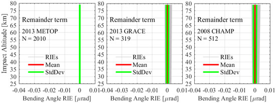
Figure 12.
Profiles and their statistics of the BNe remainder term (rightmost term of Equation (11)) for the global ensemble data sets of MetOp-A/-B missions on 15 May and 15 July 2013 (left panel), GRACE mission on 15 May and 15 July 2013 (middle panel), and CHAMP mission on 14–16 July 2008 (right panel), respectively. In each subpanel, the individual bending angle RIEs (gray), their mean (heavy red), and their standard deviation (heavy green) are shown.
Furthermore, we recall the interesting feature from Figure 10 that the EDT BNe terms and their mean values of the low-LEO-altitude missions exhibit differences, with the 2008 GRACE EDT BNe terms showing an opposite sign (plus) compared to the 2008 CHAMP and 2013 GRACE ones (minus). This can be explained by the general orientation of the geomagnetic dipole field in combination with where the satellite orbits were located on the test days, combined with the fact that both GRACE and CHAMP observe only setting occultations.
That is, on a given day, when the LEO satellite passes over the EDT region, all the GNSS satellites in occultation are predominantly viewed in the anti-velocity direction, more or less either along or against the geomagnetic field lines, along if the satellite crosses the EDT region from north to south, against if it crosses from south to north. If the orbital node changes over time (i.e., the orbit is not sun-synchronous), the LEO satellite eventually (on another day) crosses the EDT region in the opposite direction. To illustrate this effect, Figure 13 shows the geomagnetic field intensity parallel to the RO ray path for the 2013 and 2008 GRACE events. It can be seen that the geomagnetic field intensity of the 2008 GRACE EDT region events (blue curves) has the opposite sign compared to the 2013 GRACE data. This eventually causes the opposite sign of BNe terms.
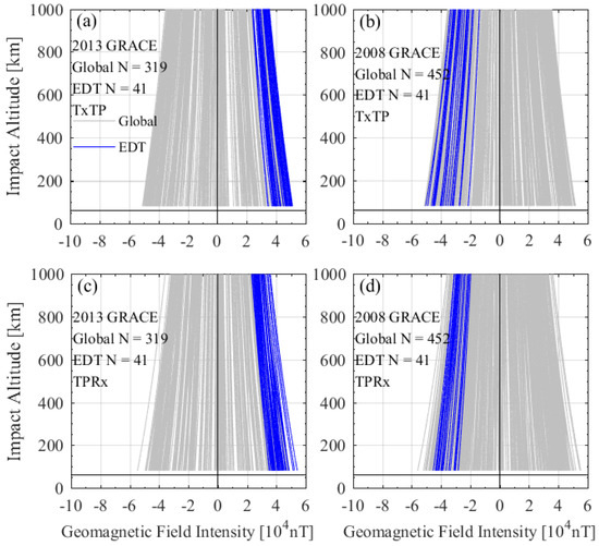
Figure 13.
Vertical profiles of geomagnetic field intensity parallel to the RO ray path for the 2013 GRACE (15 May and 15 July 2013; (a,c)) and 2008 GRACE (14–16 July 2008; (b,d)) ensemble data sets. RO events are shown as “bundle plot”, with grey profiles and blue profiles for the global and EDT regions, respectively.
Given these results, we can indeed draw the conclusion that the sign of the magnetic-field term (which depends on the angle between the geomagnetic field vector and the ray path direction) clearly affects the total BNe term. This implies that the EDT region, with its high level of ionization, is particularly important for regional RIEs. This regional-scale behavior can be captured by the bi-local correction while the simpler Kappa correction cannot account for it, due to not including the geomagnetic term.
5. Conclusions
Based on an implementation of the bi-local and the Kappa bending angle RIE correction approaches in the rOPS system, a first detailed evaluation and statistical added value analysis has been performed between these two higher-order ionospheric correction approaches for RO bending angle profiles. The study showed that the newly introduced bi-local approach performs reasonably, and in many aspects is similar to the simpler Kappa approach, particularly for large-scale averages, although important differences have been revealed.
General conclusions that can be drawn from this study are that (1) the total bending angle RIEs clearly increase with increasing solar activity, overall well captured both by the bi-local and Kappa approaches, which also is consistent with previous studies; (2) for all tested RO mission data sets, the mean bi-local Ne2 term has a clear negative tendency, an aspect where bi-local and Kappa approaches are closely consistent; (3) apart from some outliers, the bi-local RIE corrections are somewhat larger than those of the Kappa correction, while the mean profiles are often reasonably close. Thus, the bi-local approach and the smart simplified setup of the Kappa approach are, in this sense, in reasonably good agreement.
Following these general conclusions, specifics learned from the performance and added value of the bi-local correction relative to the Kappa correction are (4) in the three components of the bi-local bending angle RIE correction, the Ne2 term plays a dominant role, and the geomagnetic term (BNe term) can be important regionally; (5) for all the RO missions, the magnitude of the local-LEO (NeL) term is very small and can be neglected; (6) the bi-local approach has more capacity and clear added value, compared to the Kappa correction, to represent the variability of the ionospheric and geomagnetic conditions that affect RO events. This is particularly important for regional-scale averages, where the geomagnetic term is of key relevance, which is not accounted for by the Kappa approach.
Following up on these encouraging first results, several next steps might be taken to further improve ionospheric correction in future. That is, further analysis of the bi-local correction may investigate the following aspects, among others: (1) analyze the bi-local RIE terms further using more multi-missions data (also Constellation Observing System for Meteorology, Ionosphere, and Climate (COSMIC), Fengyun-3C/-3D (FY-3C/-3D), etc.); (2) further cross-evaluation of the bi-local approach with Kappa approach and standard correction, including large-ensemble correction validation attempts using best-available independent reference datasets (e.g., from Michelson Interferometer for Passive Atmospheric Sounding, MIPAS); (3) analyze the impact of RIEs, and particularly the impact of their correction, on level two data, i.e., retrieved atmospheric profiles such as refractivity and temperature, and explore the benefit for subsequent weather and climate applications.
Author Contributions
Conceptualization, C.L., G.K. and S.S.; methodology, C.L., G.K. and S.S.; software, C.L. and M.S.; validation, C.L., J.D. and M.S.; formal analysis, C.L.; investigation, C.L., G.K. and S.S.; resources, G.K. and Y.S.; writing—original draft preparation, C.L.; writing—review and editing, G.K. and S.S.; visualization, C.L. and G.K.; supervision, G.K. and S.S.; project administration, C.L., G.K. and Y.S. All authors have read and agreed to the published version of the manuscript.
Funding
This research was partially funded by the National Natural Science Foundation of China (grant nos. 41775034, 41405039 and 41606206), the Youth Innovation Promotion Association of the Chinese Academy of Sciences (grant no. 2019151), the Strategic Priority Research Program of Chinese Academy of Sciences (grant no. XDA15021002), the Youth Talents Program Foundation of Beijing Organization Department (grant no. 2018000097607G380) and the FengYun-3 (FY-3) Global Navigation Satellite System Occultation Sounder (GNOS) development and manufacture project led by NSSC, CAS. S.S. was supported by the Radio Occultation Meteorology Satellite Application Facility (ROM SAF), which is a decentralized operational RO processing center of the European Organisation for the Exploitation of Meteorological Satellites (EUMETSAT). The research at WEGC/University of Graz was supported by the EUMETSAT ROM SAF project VS34 and the Austrian Research Promotion Agency (FFG) projects ATROMSAF1 (ASAP-13 project no. 859771) and CLIMRECORD (ASAP-14 project no. 866020), as well as the Austrian Science Fund (FWF) project NEWCLIM (T 757-N29).
Acknowledgments
The authors thank Sean Healy (ECMWF Reading, UK) and Kent Lauritsen (DMI Copenhagen, DK) for valuable discussions and Josef Innerkofler (WEGC/University of Graz, AT) for valuable support in rOPS software developments relevant to this study.
Conflicts of Interest
The authors declare no conflict of interest.
References
- Melbourne, W.G.; Davis, E.S.; Duncan, C.B.; Hajj, G.A.; Hardy, K.R.; Kursinski, E.R.; Meehan, T.K.; Young, L.E.; Yunck, T.P. The Application of Spaceborne GPS to Atmospheric Limb Sounding and Global Change Monitoring; JPL Publication 94-18; Jet Propulsion Laboratory: Pasadena, CA, USA, 1994; p. 147. [Google Scholar]
- Kursinski, E.R.; Hajj, G.A.; Schofield, J.T.; Linfield, R.P.; Hardy, K.R. Observing earth’s atmosphere with radio occultation measurements using the global positioning system. J. Geophys. Res. 1997, 102, 23429–23465. [Google Scholar] [CrossRef]
- Steiner, A.K.; Lackner, B.C.; Ladstädter, F.; Scherllin-Pirscher, B.; Foelsche, U.; Kirchengast, G. GPS radio occultation for climate monitoring and change detection. Radio Sci. 2011, 46, RS0D24. [Google Scholar] [CrossRef]
- Lackner, B.C.; Steiner, A.K.; Hegerl, G.C.; Kirchengast, G. Atmospheric climate change detection by radio occultation data using a fingerprinting method. J. Clim. 2011, 24, 5275–5291. [Google Scholar] [CrossRef]
- Anthes, R.A.; Rocken, C.; Kuo, Y.H. Applications of COSMIC to meteorology and climate. Terr. Atmos. Ocean. Sci. 2000, 11, 115–156. [Google Scholar] [CrossRef]
- Gobiet, A.; Kirchengast, G. Advancements of global navigation satellite system radio occultation retrieval in the upper stratosphere for optimal climate monitoring utility. J. Geophys. Res. 2004, 109, D24110. [Google Scholar] [CrossRef]
- Sun, Y.Q.; Bai, W.H.; Liu, C.L.; Liu, Y.; Du, Q.F.; Wang, X.Y.; Yang, G.L.; Liao, M.; Yang, Z.D.; Zhang, X.X.; et al. The Fengyun-3c radio occultation sounder GNOS: A review of the mission and its early results and science applications. Atmos. Meas. Tech. 2018, 11, 5797–5811. [Google Scholar] [CrossRef]
- Buontempo, C.; Jupp, A.; Rennie, M. Operational NWP assimilation of GPS radio occultation data. Atmos. Sci. Lett. 2008, 9, 129–133. [Google Scholar] [CrossRef]
- Healy, S.B. Forecast impact experiment with GPS radio occultation measurements. Geophys. Res. Lett. 2005, 32. [Google Scholar] [CrossRef]
- Vorobev, V.V.; Krasilnikova, T.G. An estimation of accuracy of the atmospheric refractive-index recovery from measurements of doppler shifts at frequencies used in the navstar system. Izv. Fiz Atmos. Okeana 1994, 29, 626–633. [Google Scholar]
- Hoque, M.M.; Jakowski, N. Ionospheric bending correction for GNSS radio occultation signals. Radio Sci. 2011, 46, RS0D06. [Google Scholar] [CrossRef]
- Liu, C.L.; Kirchengast, G.; Sun, Y.Q.; Bai, W.H.; Du, Q.F.; Wang, X.Y.; Meng, X.G.; Wang, D.W.; Cai, Y.R.; Wu, D.; et al. Study of bending angle residual ionosphric error in real RO data. Int. Geosci. Remote Sens. 2016, 4171–4174. [Google Scholar]
- Mannucci, A.J.; Ao, C.O.; Pi, X.; Iijima, B.A. The impact of large scale ionospheric structure on radio occultation retrievals. Atmos. Meas. Tech. 2011, 4, 2837–2850. [Google Scholar] [CrossRef]
- Liu, C.L.; Kirchengast, G.; Zhang, K.F.; Norman, R.; Li, Y.; Zhang, S.C.; Carter, B.; Fritzer, J.; Schwaerz, M.; Choy, S.L.; et al. Characterisation of residual ionospheric errors in bending angles using GNSS RO end-to-end simulations. Adv. Space Res. 2013, 52, 821–836. [Google Scholar] [CrossRef]
- Liu, C.L.; Kirchengast, G.; Zhang, K.; Norman, R.; Li, Y.; Zhang, S.C.; Fritzer, J.; Schwaerz, M.; Wu, S.Q.; Tan, Z.X. Quantifying residual ionospheric errors in GNSS radio occultation bending angles based on ensembles of profiles from end-to-end simulations. Atmos. Meas. Tech. 2015, 8, 2999–3019. [Google Scholar] [CrossRef]
- Syndergaard, S. On the ionosphere calibration in GPS radio occultation measurements. Radio Sci. 2000, 35, 865–883. [Google Scholar] [CrossRef]
- Healy, S.B.; Culverwell, I.D. A modification to the standard ionospheric correction method used in GPS radio occultation. Atmos. Meas. Tech. 2015, 8, 3385–3393. [Google Scholar] [CrossRef]
- Danzer, J.; Healy, S.B.; Culverwell, I.D. A simulation study with a new residual ionospheric error model for GPS radio occultation climatologies. Atmos. Meas. Tech. 2015, 8, 3395–3404. [Google Scholar] [CrossRef]
- Bassiri, S.; Hajj, G.A. Higher-order ionospheric effects on the GPS observables and means of modeling them. Adv. Astronaut. Sci. 1993, 82, 1071–1086. [Google Scholar]
- Hoque, M.M.; Jakowski, N. Higher order ionospheric propagation effects on GPS radio occultation signals. Adv. Space. Res. 2010, 46, 162–173. [Google Scholar] [CrossRef]
- Danzer, J.; Scherllin-Pirscher, B.; Foelsche, U. Systematic residual ionospheric errors in radio occultation data and a potential way to minimize them. Atmos. Meas. Tech. 2013, 6, 2169–2179. [Google Scholar] [CrossRef]
- Qu, X.C.; Li, Z.H.; An, J.C.; Ding, W.W. Characteristics of second-order residual ionospheric error in GNSS radio occultation and its impact on inversion of neutral atmospheric parameters. J. Atmos. Sol. Terr. Phys. 2015, 130, 159–171. [Google Scholar] [CrossRef]
- Zeng, Z.; Sokolovskiy, S.; Schreiner, W.; Hunt, D.; Lin, J.; Kuo, Y.H. Ionospheric correction of GPS radio occultation data in the troposphere. Atmos. Meas. Tech. 2016, 9, 335–346. [Google Scholar] [CrossRef]
- Zeng, Z.; Sokolovskiy, S. Effect of sporadic E clouds on GPS radio occultation signals. Geophys. Res. Lett. 2010, 37, L18817(1–5). [Google Scholar] [CrossRef]
- Angling, M.J.; Elvidge, S.; Healy, S.B. Improved model for correcting the ionospheric impact on bending angle in radio occultation measurements. Atmos. Meas. Tech. 2018, 11, 2213–2224. [Google Scholar] [CrossRef]
- Liu, C.L.; Kirchengast, G.; Sun, Y.Q.; Zhang, K.F.; Norman, R.; Schwaerz, M.; Bai, W.H.; Du, Q.F.; Li, Y. Analysis of ionospheric structure influences on residual ionospheric errors in GNSS radio occultation bending angles based on ray tracing simulations. Atmos. Meas. Tech. 2018, 11, 2427–2440. [Google Scholar] [CrossRef]
- Danzer, J.; Schwaerz, M.; Kirchengast, G.; Healy, S.B. Sensitivity analysis and impact of the Kappa-Correction of residual ionospheric biases on radio occultation climatologies. Earth Space Sci. 2020, 7. [Google Scholar] [CrossRef]
- Syndergaard, S.; Kirchengast, G. A bi-local estimation approach for residual ionospheric correction of radio occultation bending angles. Presented at EUMETSAT ROM SAF-IROWG International Workshop, Elsinore, Denmark, 19–25 September 2019; Fri, 20 Sep; Poster P23. Available online: http://www.romsaf.org/romsaf-irowg-2019/en/content/21/program-agenda-by-day (accessed on 8 September 2020).
- Leitinger, R.; Kirchengast, G. Easy to use global and regional ionospheric models—A report on approaches used in Graz. Acta Geodaet. Geophys. Hung. 1997, 32, 329–342. [Google Scholar]
- Thébault, E.; Finlay, C.C.; Beggan, C.D.; Alken, P.; Aubert, J.; Barrois, O.; Bertrand, F.; Bondar, T.; Boness, A.; Brocco, L.; et al. International geomagnetic reference field: The 12th generation. Earth Planets Space 2015, 67. [Google Scholar] [CrossRef]
- Feltens, J. The international GPS service (IGS) ionosphere working group. Adv. Space Res. 2003, 31, 635–644. [Google Scholar] [CrossRef]
- Petrie, E.J.; Hernández Pajares, M.; Spalla, P.; Moore, P.; King, M.A. A review of higher order ionospheric refraction effects on dual frequency GPS. Surv. Geophys. 2011, 32, 197–263. [Google Scholar] [CrossRef]
- Kirchengast, G.; Schwärz, M.; Schwarz, J.; Scherllin-Pirscher, B.; Pock, C.; Innerkofler, J.; Proschek, V.; Steiner, A.K.; Danzer, J.; Ladstädter, F.; et al. The reference occultation processing system approach to interpret GNSS radio occultation as SI-traceable planetary system refractometer. Presented at OPAC-IROWG International Workshop, Leibnitz, Austria, 8–14 September 2016; Available online: http://wegcwww.unigraz.at/opacirowg2016/data/public/files/opacirowg2016_Gottfried_Kirchengast_presentation_261.pdf (accessed on 8 September 2020).
- Kirchengast, G.; Schwärz, M.; Angerer, B.; Schwarz, J.; Innerkofler, J.; Proschek, V.; Ramsauer, J.; Fritzer, J.; Scherllin-Pirscher, B.; Rieckh, T.; et al. Reference OPS DAD—Reference Occultation Processing System (rOPS) Detailed Algorithm Description; Technical Report for ESA and FFG No. 1/2018, Doc-Id: WEGC-rOPS-2018-TR01, Issue 2.0; Wegener Center, University of Graz: Graz, Austria, 2018. [Google Scholar]
- Schwarz, J. Benchmark Quality Processing of Radio Occultation Data with Integrated Uncertainty Propagation; Scientific Report No. 77-2018; Wegener Center Verlag: Graz, Austria, 2018. [Google Scholar]
- Schwarz, J.; Kirchengast, G.; Schwärz, M. Integrating uncertainty propagation in GNSS radio occultation retrieval: From excess phase to atmospheric bending angle profiles. Atmos. Meas. Tech. 2018, 11, 2601–2631. [Google Scholar] [CrossRef]
- Gorbunov, M.E.; Kirchengast, G. Uncertainty propagation through wave optics retrieval of bending angles from GPS radio occultation: Theory and simulation results. Radio Sci. 2015, 50, 1086–1096. [Google Scholar] [CrossRef]
- Gorbunov, M.E.; Kirchengast, G. Wave-optics uncertainty propagation and regression-based bias model in GNSS radio occultation bending angle retrievals. Atmos. Meas. Tech. 2018, 11, 111–125. [Google Scholar] [CrossRef]
- Schwarz, J.; Kirchengast, G.; Schwärz, M. Integrating uncertainty propagation in GNSS radio occultation retrieval: From bending angle to dry-air atmospheric profiles. Earth Space Sci. 2017, 4, 200–228. [Google Scholar] [CrossRef]
- Li, Y.; Kirchengast, G.; Scherllin-Pirscher, B.; Schwärz, M.; Nielsen, J.K.; Ho, S.P.; Yuan, Y.B. A new algorithm for the retrieval of atmospheric profiles from GNSS radio occultation data in moist air and comparison to 1DVar retrievals. Remote Sens. 2019, 11, 2729. [Google Scholar] [CrossRef]
- Innerkofler, J.; Kirchengast, G.; Schwärz, M.; Pock, C.; Jäggi, A.; Andres, Y.; Marquardt, C. Precise orbit determination for climate applications of GNSS radio occultation including uncertainty estimation. Remote Sens. 2020, 12, 1180. [Google Scholar] [CrossRef]


Publisher’s Note: MDPI stays neutral with regard to jurisdictional claims in published maps and institutional affiliations. |
© 2020 by the authors. Licensee MDPI, Basel, Switzerland. This article is an open access article distributed under the terms and conditions of the Creative Commons Attribution (CC BY) license (http://creativecommons.org/licenses/by/4.0/).