Abstract
Reliable and accurate positioning underwater has been the goal of many research activities in the last years. In this paper, we present our design of a self-maintainable underwater navigation system, which provides a simple, low-cost, and flexible solution. In our concept, a set of buoys is equipped with Global Navigation Satellite System (GNSS) receivers as well as underwater pseudolite signal transmitters. Therefore, the buoys are able estimate their position and transmit this information underwater through a pseudolite signal. We particularly designed this signal for underwater ranging for both fresh and salt water. Any suitable underwater receiver is then able to do ranging via these pseudolite signals. In this paper, we theoretically analyze and test our concept using several buoy distributions and diving depths. The optimal arrangement of buoys is determined in terms of accuracy and availability depending on the number of available buoys and targeted water depth for an efficient operation. For example, at a targeted depth of 30 m in fresh water, a maximum horizontal position root-mean-square (RMS) error of less than 3 m can be achieved with a set of five buoys providing a service radius of up to 72 m.
1. Introduction
A reliable and accurate underwater positioning is mandatory for divers, as well as underwater vehicles [1]. In the past, many different approaches have been proposed and most of them are based on acoustic underwater positioning system [2,3,4,5] or using optical signals [6]. Acoustic waves are mostly used for underwater ranging in salt water as electromagnetic waves are strongly attenuated. Only short ranges are achieved with electrometric waves compared to the ones obtained by acoustic waves, and hence, they are not suitable for underwater ranging methods [7]. A system for the tracking and navigation of underwater vehicles or divers through acoustic distance, or direction measurements, and subsequently by position triangulation can be found in [8]. The measurements are based on a sea-floor baseline transponder network, which limits the area of the system’s operation. Depending on the baseline length, there are three broad types: Long Baseline (LBL) System, Ultra Short Baseline (USBL) System, and Short Baseline (SBL) System. Though acoustic waves have clear advantages in low underwater attenuation, they also have some significant drawbacks. They are complex, and many acoustic systems cannot be exported as they are subject to technological restrictions imposed by the respective governments. Acoustic systems are also sensitive to noise, and due to low diffraction suffer from shadow zones created by large objects or seafloor topography. Furthermore, acoustic links can be significantly affected by multipath propagation due to reflection and refraction in shallow water [9]. In addition, acoustic systems increase the underwater noise level and therefore may have a negative impact on underwater mammals [10].
An underwater 3D mapping system for divers is described in [11]. It combines data from different instruments a scuba diver normally uses to find its position. A boat or another point of interest can be used as a reference. The most important innovative part of this system is the wireless data signal that works well underwater. In addition, an independent underwater vehicle can be used in 3D environment modeling for underwater navigation visual odometry [12]. A review of underwater communication systems can be found in [13].
Global Navigation Satellite Systems are widely used. Typically, navigation systems can be divided into various categories based upon their applications such as land (e.g., car, pedestrian, bicycle, rail), maritime, and aeronautical. In maritime navigation, we usually discuss the aspects of moving object or vehicles navigating on the surface of the water. The inability to use GNSS signals in underwater is a drawback [14]. The reasons are the low power of the received satellite signal and their high attenuation in an aquatic environment. Hence, GNSS cannot be directly used for underwater navigation. Enabling the GNSS technology also for underwater applications has a very lucrative market potential.
A simple way to facilitate GNSS for effective underwater navigation is by using a floating GNSS antenna on the water surface connected to the underwater user through a cable. The length of the cable line (maximum depth restriction) and not able to position the antenna exactly above the user, which affect the accuracy, are limitations of the solution [15,16].
Another way to determine the position of an underwater object is by using a GPS Intelligent Buoys (GIB) system [17]. GIB may be classified as inverted LBL devices in which the transducers are installed on GPS equipped sonobuoys. Typically, the sound source or impact event is tracked or localized using a time of arrival technique (TOA). GIB systems are used to track Autonomous Underwater Vehicles (AUVs), torpedoes, or divers. They can also be used to detect airplanes’ black-boxes by localization [18].
A further interesting underwater navigation system solution using acoustic waves with range up to 250 m can be found in [19]. It uses only one buoy whose position is connected to a GPS antenna on land with a Real Time Kinematic (RTK) system or Satellite-Based Augmentation System (SBAS). The movement of the buoy is modeled using a Motion Reference Unit (MRU) gyroscope and a Kalman filter. To perform optimally, this system requires an RTK station nearby, which might be not feasible in an open-water scenario and so MRU is also quite complex.
In contrast, our system is of low cost and does not involve any complex computations. Our system consists of two parts: first, the terrestrial localization of each buoy by using GNSS, and second, the localization underwater by exploiting electromagnetic signals transmitted by each buoy. Each buoy serves as a pseudolite (a device working like a satellite, but not placed in orbit). The first part, the GNSS localization is well-known in the community and is not investigated in this paper. Its implementation can be easily done and maintained with commercial-off-the-shelf (COTS) products. For the second part, we have designed an electromagnetic signal suitable for the proposed application. This signal is used for one-way ranging between the buoy’s transmitter and underwater receiver. Additionally, we apply a triangulation method with theses ranges to obtain the underwater position. Our presented system is flexible and constructed such that it can be applied to both fresh and salt water environment. This paper contains a preliminary theoretical study of our concept, which is introduced and discussed for the first time.
The paper is organized as follows: First, we introduce our system concept and then discuss the selected design aspects of the chosen underwater signal and its ranging properties. Then, we describe the choice of navigation frequency and the antennas that are used to send the navigation signal underwater followed by the expected underwater position accuracy based on the performance of the GNSS receivers and underwater ranging error propagation based on our chosen underwater ranging method. By selecting realistic simulation parameters, we analyze the position performance of different buoy distributions in terms of accuracy and availability. We discuss these results and extract the optimal distancing of buoys in order to provide a maximum service area while maintaining an underwater position standard deviation of less than three meter. This discussion is done for several numbers of available buoys and water depths of operation. Finally, we outline the conclusions of our findings.
2. Materials and Methods
The concept of our mobile underwater radio-navigation system using pseudolite buoys is a new approach to solve the underwater navigation problem. The system can be split in two parts: the terrestrial localization of each buoy using GNSS, and the underwater localization applying triangulation on pseudolite signals transmitted by each buoy underwater. A scheme of its operation is presented in Figure 1.
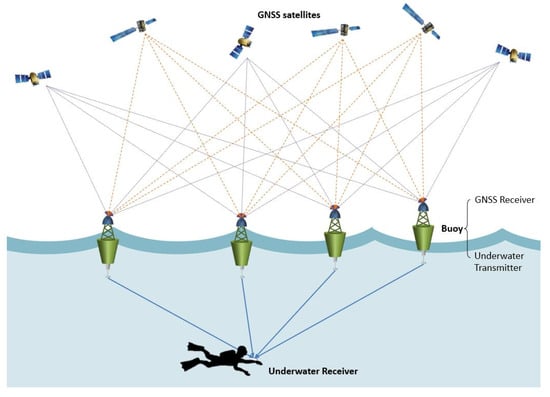
Figure 1.
Illustration of the mobile underwater radio-navigation system using the pseudolite buoys concept.
The key device is a buoy equipped with a dual-frequency, multi-constellation GNSS antenna and receiver on the top and a pseudolite signal transmitter on the bottom. A set of at least three buoys creates the needed aquatic environment needed for our investigations. The buoy’s GNSS receiver determines its position in real time based on dual-frequency, multi-constellation GNSS data. The required antenna and receiver can be COTS products.
The goal of our system was to achieve underwater position accuracy within a standard deviation lower than 3 m. The developed navigation system should be portable and low cost. The underwater navigation system should preferably use electromagnetic waves instead of acoustic waves so that they should have a low impact on underwater mammals. At the very least, the rapid attenuation of electromagnetic waves in water prevents any harm to mammals which are outside the service volume of the proposed system. Nevertheless, the principles of the proposed concept can also be utilized for systems with higher accuracy requirements and acoustic signals.
2.1. Underwater Signal Design and Ranging
The signal transmitted by each buoy must essentially fulfill two tasks. First, it must allow precise measurement of the distance (range) it has traveled from the buoy to the user’s antenna. Second, it should carry the necessary data bits, which provide information about the buoy’s coordinates. Ranges and buoys’ coordinates are combined by the user to determine its position in an absolute coordinate frame.
Signal propagation conditions of a medium as challenging as water are taken into account when designing a reliable navigation signal system. In the following, we discuss and selection of suitable navigation frequencies in the Low Frequency (LF) / Ultra Low Frequency (ULF) bands. Our design takes into account the propagation of electromagnetic (EM) waves in water at various frequencies and the predominant noise sources in water based upon the comprehensive overview on underwater radio signals by Moore [20]. A brief review of the relevant propagation and noise characteristics is provided in the Appendix A and Appendix B of this paper.
2.1.1. Choice of Navigation Frequency and Bandwidth
The signal propagation characteristics given in Appendix A suggest that underwater EM waves are not an attractive option for use as they generally require large antenna systems, high power, and very low frequencies [16,17]. The need for usage of very low frequencies limit the selection of possible bandwidths and data transfer rates: since higher frequencies are attenuated significantly more than lower frequencies and the transmitted signal that does not have a very narrow bandwidth will arrive in a distorted form at the receiver. Clearly, a signal such as the GPS L1 C/A code containing all frequencies from 0–1 MHz could not be transmitted or retransmitted by a buoy as some frequencies would be attenuated significantly more than others, and the received signal would be an extremely distorted one. Instead, a very simple navigation signal with a narrow bandwidth should be targeted, which transmits only a few bits per second.
When choosing the preferable transmit frequency for a system such as ours, certain difficulties are faced: on the one hand, signals with short wavelengths are undesirable because of their strong attenuation. In a conducting medium, transmitting the signals over the distance of several wavelengths is not at all possible [16]. On the other hand, using a large wavelength may be a better option due to weaker attenuation, but larger antennas will be required. As an intermediate solution, we decided to use the moderate wavelength λ = 50.0 m (equivalently, a skin depth of δ = 7.96 m). Depending on the type of water, this corresponds to a frequency of fU = 1.0 kHz (sea water/ULF) and fV = 80.0 kHz (fresh water/LF). For these frequencies, attenuation is still acceptable (1.09 dB/m) and far-field assumptions such as shown in Equation (A1) can serve as a first-order approximation.
2.1.2. Pilot Signal and Ranging Accuracy
Ranging in GPS is classically achieved by estimating the navigation signal’s time-delay, which it experienced when travelling through space. Time-delay estimation is done by detecting rising or falling signal edges of a known code sequence (pilot) and comparing them to a local reference. The accuracy of such code-delay-based ranging depends on the "sharpness" of the rising and falling signal edges, hence on the signal bandwidth. The approximate order of magnitude of achievable ranging accuracy is given by c/B, where c is the speed of light and B is the signal bandwidth. For the 1 MHz L1 C/A signal, this conforms to 300 m. Obviously, an underwater EM signal with bandwidth of the order of Hz or even kHz does not result in sufficient accuracy.
We propose ranging based on the signal amplitude instead of the signal delay as a solution. We exploit a simple principle: the lower the received signal power, the further away the signal source. Unlike in free space, the amplitude attenuation of a received waveform is a strong indicator of the range r it has travelled. Amplitude decreases only with in air or vacuum, but with in a conducting medium such as water, where δ is the medium’s skin depth.
Consider the signal block diagram in Figure 2.
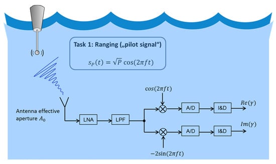
Figure 2.
Pilot signal and receiver’s signal processing.
The buoy’s pilot signal is represented by
with the effective transmit power P and ω = 2πf, with the technical frequency f as selected in Section 2.1.1. We identify the range-dependent attenuation and phase in Equation (A1):
Notably, the phase also carries information about the unknown range, which we shall exploit. Now, the signal received by an antenna with receiving cross-section (or effective aperture) A0 (in units of m2) located at a distance r from the transmitter can be expressed as:
The unknown term is any kind of interference, which is mainly atmospheric noise. After passing through a low-noise amplifier (LNA), the signal is low-pass filtered with bandwidth and is converted from its carrier frequency to an in-phase/quadrature (I/Q) baseband signal. We assume that the complex-valued baseband signal is sampled with a high-resolution logarithmic quantization analog-to-digital (A/D) converter during an observation interval of length T0
where w(t) is now a complex-valued zero-mean noise process. Typical noise levels in the relevant LF/ULF band are briefly discussed in Appendix B. For simplicity, we assume proper Gaussian atmospheric noise with power spectral density N0
We use the EXtended Invariance Principle (EXIP) of maximum likelihood estimation to estimate r from (r, t) in a two-step approach.
- Estimation of the complex phasor . The maximum likelihood estimator is given by:
- It is realized in digital signal processing by using an integrate-and-dump (I&D) filter. Now the range r from is estimated. The maximum likelihood estimator is given by:
A graphic interpretation of this approach is shown in Figure 3 in the form of a Nyquist plot (location curve) in logarithmic polar coordinates. The two outputs from the digital signal processing are shown in Figure 2: Re(γ) and Im(γ) can be mapped to a polar plot with phase and amplitude. The receiver will estimate the range depending on nature of the two outputs. Each traveled wavelength corresponds to one complete circle of 360°, and the phase ambiguity can be resolved via the amplitude. As a noisy measurement will typically never synchronize with the shown curve, a criterion such as Equation (7) is necessary to obtain the range estimate. When many noisy measurements are available, they can be averaged to increase accuracy.
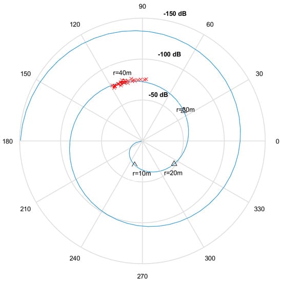
Figure 3.
Logarithmic amplitude 20log10(r) in dB and phase (r) in degrees, for ranges from 0–100 m and noisy measurements received by a receiver at 40 m.
The EXIP states that for sufficiently long observation times T0 (long averaging), the above two-step approach has the same performance as a direct (but computationally costly) estimation of the range from the received signal. The variance of the range estimate is given by:
This means that the ranging accuracy is dependent on the range itself: it is more difficult to get range estimation from a faraway buoy. The standard deviation (“accuracy”) of ranging is given by .
In Table 1 we suggest a set of meaningful/feasible system parameters and the accuracy is plotted as a function of distance in Figure 7.

Table 1.
Values of system parameters and physical constants.
It can be seen that good ranging accuracy (on the order of a few meters) is possible for ranges up to 90 m. For smaller ranges r < λ, the figure suggests that millimeter accuracy is possible. However, in this case, far-field conditions are clearly violated so that these results are overoptimistic and should be interpreted with care. However, we can state at this point that ranging with our system is theoretically feasible.
Finally, note from Equation (8) that a trade-off between transmit power and observation time can be made. The power can be reduced at the cost of a longer time ; hence, a slower dynamic response of the system.
2.1.3. Data Signal and Bit-Error-Probability
To transmit the necessary bits containing the buoy’s absolute position in the GPS coordinate frame, we transmit a second signal given by:
Pilot and data signals do not interfere due to the orthogonality of sine and cosine. The phase of the sine wave alternates by with a rate of 1/Tb, where Tb is the bit duration, depending on whether a binary 0 or 1 is transmitted. The data signal and the necessary receiver’s signal processing are illustrated in Figure 4. As the phase is already known from the pilot module, the data can be coherently demodulated, without using a quadrature baseband channel. The I&D filter output β is used by a hard decision device to decide which datum was transmitted. In the case β < 0, we decide for “1”, or otherwise we decide for “0”.
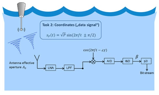
Figure 4.
Data signal and receiver’s signal processing.
From the energy per bit we can obtain the following well-known expression for bit error probability with binary phase-shift keying (BPSK) modulation:
Suppose that the buoy transmits two coordinates (in the
horizontal plane), each consisting of 12 bits. Therefore, one frame (packet) of
coordinates consists of bits. The frame error probability is just given by . Both and are shown in Figure 5, where the data rate was chosen as 3 bits/s (i.e., the 2D coordinates are transmitted and updated every 8 s, which should be enough to cover the slow buoy dynamics). All remaining parameters are as specified in Table 1. Reliable data transmission is possible up to 85 m of range with such a data rate. Again, error probabilities for ranges on the order of the wavelength may be overoptimistic.
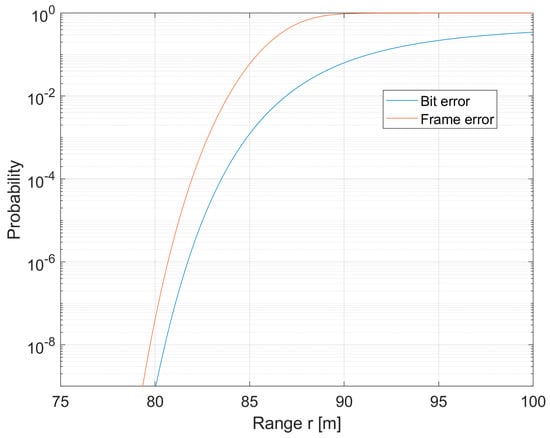
Figure 5.
Reliability of data transmission.
2.1.4. Multiple Access Strategy and Total System Bandwidth
So far, we have only considered one buoy. However, since we need multiple buoys to allow positioning in all three dimensions of space, we have to ensure that buoys do not interfere with each other. One possible strategy to avoid interference is frequency-division multiple access (FDMA) as illustrated in Figure 6.
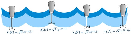
Figure 6.
Buoy links separated in frequency domain with frequency-division multiple access (FDMA).
Here, the buoys would not all use the same carrier frequency f given in Equations (A4) and (A5), but rather transmit on separate frequencies f1, f2, f3, … adjacent to f. Each buoy needs a bandwidth equal to the data rate 1/Tb plus a guard interval ±F. Then, the total range of frequencies occupied by an ensemble of K buoys is the frequency interval , with the total system bandwidth:
For instance, with and four buoys, we would have a total system bandwidth of Bs = 80 Hz.
2.2. Antennas for Underwater Communication and Frequency Allocation
The antenna length should be a fraction of the operating wavelength for an effective radiation. For the most of antennas it is half-wavelength (λ/2) or quarter wavelength (λ/4). As water has high dielectric constant and conductivity, the resulting wavelength will be much shorter than in the air for a given frequency (e.g., for an electromagnetic wave with a frequency of 10 kHz the wavelength is 30 km in space but only 15.8 m in seawater). However, as mentioned before, water is a conductive medium and to minimize very high attenuation loss of signals in water, very low frequencies (i.e., long wavelengths) must be used. A wavelength of 50 m was selected for the proposed navigation system, which results in the operating frequency of 1 kHz in seawater and 80 kHz in fresh water. For such a wavelength, even antennas with a length of a quarter of operating wavelength are too bulky for a portable system. Therefore, electrically small antennas must be used [21]. Such antennas are much shorter than the wavelength of the operating signal and are generally less efficient. They are also more challenging to design than larger full-sized antennas. Impedance matching is needed for electrically short antennas to be able to operate at 50 ohms and it can be achieved with the help of lump components. Many types of antennas for underwater applications are discussed in the literatures [22,23,24,25,26,27]. Most of them are wideband antennas for underwater communications in the MHz region; however, the basic principles of design and performance of these antennas apply also for lower frequencies in the kHz region [28]. These antennas are based mostly on loops, long wires, and dipoles. They offer bi-directional radiation pattern similar to the number "8". However, the radiation characteristics of these antennas significantly change due to conductivity of the medium, for example from freshwater to seawater and in space. Therefore, to allow for accurate range estimate, 3D radiation patterns of the chosen antenna must be simulated or measured for all relevant water environments and their influence considered in the range computations. As stated in [29], antennas which are based on magnetic field outperform electric antennas in mediums with conductivity. Therefore, loop antennas seem to be particularly attractive for underwater applications. In [9], a low loss electrically small loop antenna sealed in a waterproof box was proposed for underwater applications. Loop antennas can be built from a long bendable copper wire and shaped to a N-turn rectangular or circular loop. This shaping can be done already shortly before use allowing for efficient stowage. As the loop antennas can be made out of standard copper wire, a low-cost solution seems to be possible. More accurate estimations of the required volume and costs require extensive full-wave electromagnetic simulations and measurements and are beyond the scope of this theoretical study.
The frequency range from 8.3 kHz to 275 GHz is allocated and therefore transmission only in certain bands with specified requirements is allowed [30]. There are no such restrictions for the proposed operation frequency of 1 kHz in seawater. The second chosen frequency of 80 kHz for the operation in fresh water is allocated to maritime radio navigation and radiolocation. The amount of allowed power is not specified for this band but it is only noted, that the transmission is allowed only on condition that it does not cause harmful interference to other services to which these bands are allocated. Our system should transmit signals only underwater. However, due to radiation pattern characteristics of the used antennas, underwater propagation direction, and partially transparent water/air boundary, a small portion of the navigation signal transmitted underwater would be radiated in air. If this radiated energy is above the locally allowed power level, transmit power can be reduced without accuracy loss by extending the observation time. The proposed underwater navigation system can of course operate at frequencies lower than 80 kHz in fresh water and when some transmission restrictions cannot be met, not allocated frequencies can be used.
2.3. Underwater Positioning
In this section, the impact of the expected GNSS position accuracy of each buoy on the underwater navigation is discussed. We also derive the horizontal underwater position error and analyze possible circular setups of buoys in terms of expected horizontal position accuracy and system availability area both depending on the diving depth of the user.
2.3.1. Determination of Underwater Position Accuracy
Each buoy is equipped with a multi-constellation, dual frequency GNSS receiver, and hence, able to compute its own position. The GNSS positioning is an iterative process described detailed and repeatedly in the literature, for instance in [19]. After the self-localization, the buoy sends its position information underwater. The underwater vehicle or diver receives this transmitted signal and can extract two key points from it: (a) the estimated range to the buoy and (b) the buoys transmitted position. To compute a full 3D position independently, at least three buoys have to be within the reception range of the user. Please note that in comparison to the GNSS concept, we do not need to resolve any clock offset since the range to each buoy is estimated in a one-way manner by examine the signal amplitude attenuation at the receiver.
To solve the resulting non-linear underwater user position equations, an iteratively Weighted Least Square (WLS) algorithm is applied:
where is the geometry matrix containing in each row the transpose of all 3D Line of Sight (LoS) vectors pointing from the ith buoy to the underwater user. The underwater vector’s range error is denoted by and is composed of two main sources: one resulting from the uncertainty of the ith buoy’s own position and one caused by the underwater propagation of signal from the ith . Both error sources are discussed below in detail.
2.3.2. Impact of GNSS Position Error
The first component, the GNSS buoy position error, which maps onto the underwater range error, can be expressed as:
Thus, one dimensional range error that results after mapping 3D GNSS position error of the kth buoy onto the underwater range. In case N buoys are within the maximum range of reception, the range error vector due to the individual GNSS position errors can be expressed as:
To protect the GNSS performance, two assumption are made: First, the selection of the GNSS antenna and mounting of the antenna are done such that GNSS signal reflection from the water surface are suppressed and they do not affect GNSS ranging. Second, we assume the usage of GNSS fault detection and exclusion methods. Therefore, faulty GNSS signal can be detected and are not used for the buoy’s localization. Therefore, we can expect that the remaining GNSS errors can be modeled as a Gaussian distributed random variable with zero mean and variance matrix . It is assumed that all buoys are equipped with the same GNSS receiver and antenna, and they see the same set of satellites with same satellite geometry (i.e., they are placed relatively close). In addition, we can say that all buoys experience the same GNSS position uncertainty, and so, their GNSS position covariance matrix can be assumed to be identical: as a consequence, we can formulate the range covariance matrix based on the GNSS position error as:
Please note that each buoy transmits its position and associated position error covariance matrix within the underwater signal range. However, the GNSS clock error will not affect the underwater range error.
2.3.3. Impact of Underwater Signal Propagation Range Error
The second error component is caused by the underwater signal propagation. The error related to the underwater signal propagation depends mainly on the travelled distance of the signal. For simplicity, we will assume a perfectly homogeneous medium, although the permittivity may vary slightly with temperature and pressure, and although water currents may change salinity locally.
Thus, the underwater ranging error can be assumed to follow a Gaussian distribution with zero mean and variance . Recall Equation (8), we can express this term as
where is the traveled distance underwater, is a constant factor and δ is skin depth in meter. Additional information on the ranging error can be found in Appendix A. We also assume that the underwater signal transmitter is the same for all buoys, i.e., . The covariance matrix of the underwater propagation error is given by:
Figure 7 illustrates the standard deviation of this error over the traveled distance. As it can be seen, for a distance larger than 30 m the standard deviation increases exponentially. For ranges above 80 m, the deviation is bigger than 1 m. This means that the position performance decreases significantly with ranges larger than 80 m. To limit the propagation range error, we have selected a maximum range of 100 m for our investigations. Therefore, we bound the standard deviation of the propagation range error to a maximum of 20 m.
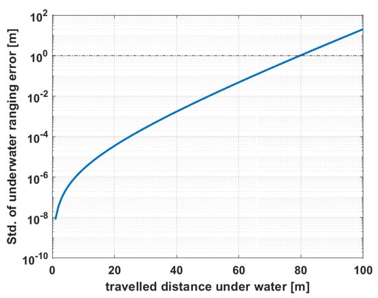
Figure 7.
Evolution of the standard deviation of the underwater ranging error for and δ = 7.96 m. Please note that the standard deviation is plotted logarithmic and the dashed line indicates a m.
Please note that a precise clock might affect this type of ranging error as it will lead to a more precise and stable complex phasor estimation.
Putting everything together in Equation (12), we can reformulate the underwater user position error equation as:
The overall underwater position error covariance matrix is then obtained by:
The underwater weighting matrix is given by:
To evaluate the overall underwater position error accuracy, we can state the underwater position covariance matrix by:
Hence, the underwater position accuracy depends mainly on the distribution of the buoys. As there will be a strong attenuation of the signal power in water, this range helps to ascertain the signal and ranging quality.
Then for evaluating the underwater position, we select the expected horizontal position standard deviation as metric of interest and it is given by:
Please note that the underwater depth of the receiver is also estimated and not constraint by any additional sensor or method. If this would be the case, the horizontal position accuracy would be even enhanced. Due to the reduction of estimation parameters, the measurement redundancy increases and the horizontal standard deviation reduces.
In order to assure a certain quality of the underwater position performance, we used the Horizontal underwater Dilution of Precision (HuDOP), which is given by
This value provides an idea of how strong the propagation of buoy’s range errors onto the underwater position solution is. The higher this value is, the higher the position error will be.
3. Results
In this section, the expected performance of the above described system is evaluated in terms of horizontal position uncertainty and expected service volume. The values for the underwater signal and water quality are assumed to be the following: a constant magnitude of and a skin depth of δ = 7.96 m. The full set of fixed underwater signal parameters is given by the Table 2.
Table 2.
Fixed simulation parameters.
Although we chose here a fresh water scenario, all provided results in this paper are also valid for a salt water scenario of an underwater signal carrier frequency of 1.0 kHz. Evidently, the location or placement of the buoys will have a major impact on the underwater performance. We investigated circular distribution of N buoys, where N-1 buoys distributed evenly on a circle of radius and one is placed in the center of the circle. An example of nine buoys is represented in Figure 8.
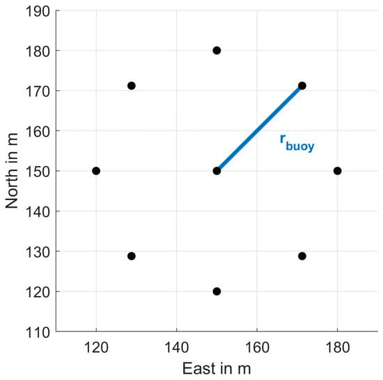
Figure 8.
Circular Distributions of N buoys with one buoy is placed in the center and all N−1 buoys are placed evenly along a circle with radius
The center of operation is located on the Lake Wessling in Germany and the georeferenced location is latitude 48.072898° N, longitude 11.250898° E, and at an altitude of 596 m. It is also illustrated in Figure 9. The maximum range of each buoy is assumed as 100 m since otherwise the underwater signals will be too attenuated to reach the underwater user. All investigations are based on GPS and Galileo constellation seen on February 14th, 2020 at 10 am UTC. This day was chosen arbitrary and serves only as an example. Appendix C will give more details about the GNSS reception.
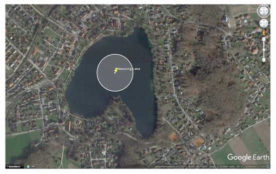
Figure 9.
Illustration of the center of operation located in the middle of Lake Wessling, Germany.
We consider the underwater positioning system as available only if the signals of at least three buoys are received at the same time by the underwater receiver. The underwater position accuracy is simulated in terms of expected horizontal position error standard deviation as described in the previous section. Different scenarios with different number of buoys and radius of buoys were analyzed. The parameters of different scenarios are presented in Table 3.
Table 3.
Variable simulation parameters.
For the following results, we only consider underwater position solutions with a HuDOP smaller or equal to 10. The expected horizontal position performance for a water depth of 30 m and buoy distribution radius of 30 m for the different numbers of buoys is illustrated in Figure 10. The locations of each buoy are indicated by a black circle. If less than three buoys are received by the user, the system is not available and the corresponding area stays white. The expected horizontal underwater position standard deviation can go up to 95 m. However, this normally only occurs on the border of the availability area. Additional results for different sets of parameters and a water depth of 30 m can be found in Appendix D. Please note that the horizontal position accuracy is limited by the accuracy of the GNSS receivers. That is, even with no underwater ranging errors, any transmitted position error of the buoys, which results from their GNSS position estimation, would propagate to an underwater position error.
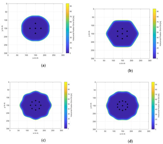
Figure 10.
Distribution of horizontal position error standard deviation in [m] at a water depth of 30 m and outer circle radius of 30 m depending on the number of buoys N: (a) N = 5, (b) N = 7, (c) N = 9, and (d) N = 11.
It is observed from the figures that the horizontal underwater position accuracy in most of the available area is below 5 m and it drops down very quickly to nearly above 70 m at the edges. The upper value of 95 m is mainly driven by the maximum allowable HuDOP value of 10. In the white areas, the system is unavailable for the underwater positioning system.
We have analyzed the performance for water depths from 1 to 100 m. The resulting averaged horizontal position accuracy for the availability area is shown Figure 11.
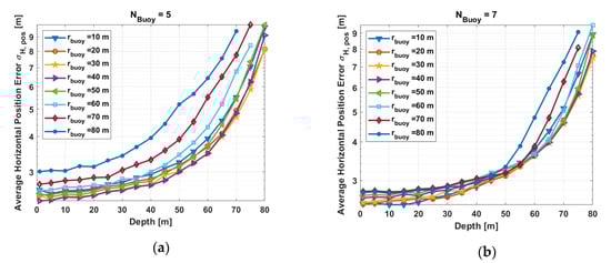
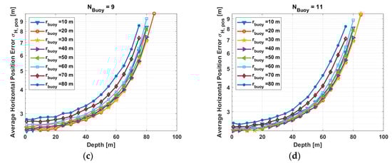
Figure 11.
Average horizontal position error standard deviation versus water depth for different radius of buoy displacement and different number of buoys: (a) N = 5, (b) N = 7, (c) N = 9, and (d) N = 11.
The different lines represent the results for different buoy circle radius indicated by the legend. It is observed that for all setups and water depths smaller than 40 m the performance is very similar and shows a similar trend. That is up to the depth of 50 m the average standard deviation is below 10 m. Below this depth the error increase will be exponential, and this highly correlates the underwater propagation error.
As one of our design goals was to achieve a maximum horizontal position error standard deviation less or equal to 3 m, we investigated in particular for this performance. In Figure 12, we see the availability area versus the water depth for all investigated setups. As it is seen, we can only provide a service with the required underwater position performance of less or equal 3 m standard deviation for water depths less than 80 m.
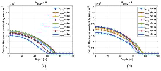
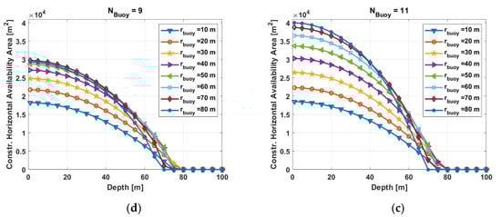
Figure 12.
Horizontal system availability area for a maximum horizontal position error standard deviation of 3 m versus water depth for different radius of buoy displacement and different number of buoys: (a) N = 5, (b) N = 7, (c) N = 9, and (d) N = 11.
4. Discussion
Our proposed system is very flexible and has low installation and maintenance costs. It is completely self-calibrating and independent. Moreover, it is world-wide deployable and operational. Based on the above provided simulation results, we are able to obtain optimal radius of the buoy circle depending on the number of available buoys and horizontal underwater position accuracy.
For example, let us have a closer look at the case of five buoys, where four are placed on a circle with radius and one at the center of the circle: From Figure 12a, we can extract the expected availability area depending on the water depth and buoy circle radius for maximum accepted horizontal position accuracy requirement in terms of standard deviation below 3 m. It is observed that the largest availability area of m² is available at 30 m water depth with a radius m. As this is difficult to picture, we introduce here the term equivalent service radius . This is the radius leading to the same availability area. In our case, it would be m.
Table 4 summarize the optimal buoy radii to obtain the maximum service area in a water depth of 30 m for different number of buoys. Additionally, the equivalent service radii are also provided. As it is stated, we can achieve a horizontal service area up to 163 m² and 341 m² for 5 buoys with 40 m radius and 11 buoys with 80 m radius are exploited, respectively. The corresponding equivalent service radii would be 72.2 m and 104.2 m.
Table 4.
Service area and corresponding service radius for a water depth of 30 m.
We also investigated the performances for different water depths. Figure 13 summarizes the equivalent service radius results for different water depths and number of buoys used. The corresponding optimal buoy circle radius is indicated by the color scale. As it can be seen depending on the number of available buoys and water depth of interest, changing the circle radius would result in the highest availability area of the system. We can extract that the deeper the operational area of interest, the smaller the optimal buoy circle radius. The results in this paper are based on theoretical studies only. They provide a first assessment on the potential of the concept. In order to further test and validate this concept, field tests would be mandatory. They would also provide a more resilient assessment of the expected system performance.
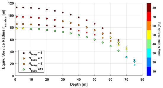
Figure 13.
Equivalent service radius versus water depth for different numbers of available buoys; the color scale indicates the optimal radius of the buoy’s outer circle.
5. Conclusions
There are many developed concepts and ready-made underwater navigation systems available. Each of them has some advantages and disadvantages based upon its construction and functioning. Our proposed solution operates on the basis of GNSS systems and underwater ranging with a cleverly designed electromagnetic signal. Our investigations show that theoretically it is possible to develop an underwater navigation system, which is flexible, low cost, and world-wide deployable and operational.
The theoretical background of our system is presented in the paper. The scientific considerations and simulations are explained in detail and characterized. A simplistic LF/ULF navigation signal is designed, which allows estimation of the buoy-terminal range with reasonable accuracy in the highly attenuating transmission medium fresh/sea water. The simulations are performed for different buoys distributions and setups. Our analyses lead to the conclusion that horizontal position accuracy in terms of standard deviation below 3 m for water depths up to 80 m is achievable. For depths higher than 80 m, we can still provide a solution, however with significant loss in accuracy. Furthermore, optimal buoy distribution for the given system requirements and the corresponding service area underwater are determined. For instance, the optimal radius of a circular distribution of 7 buoys (6 evenly distributed on the circle with this radius and one in the center) would be 80 m leading to a service area of 200 m at a water depth of 30 m.
Author Contributions
Conceptualization, A.G., C.E., L.A.G., D.T., G.G. and A.C.; Formal analysis, A.G., C.E. and L.A.G.; Funding acquisition, D.T. and G.G.; Investigation, A.G. and C.E.; Methodology, A.G., C.E., L.A.G., D.T., G.G. and A.C.; Project administration, L.A.G.; Resources, D.T., G.G. and A.C.; Software, A.G. and C.E.; Supervision, L.A.G.; Validation, A.G. and C.E.; Visualization, A.G. and C.E.; Writing—original draft, A.G., C.E. and L.A.G.; Writing—review & editing, A.G., C.E., L.A.G., D.T. and A.C. All authors have read and agreed to the published version of the manuscript.
Funding
The authors are thankful to DLR Technology Marketing for funding this research. The research was performed in the frame of European Satellite Navigation Competition (ESNC).
Conflicts of Interest
The authors declare there is no conflict of interest.
Appendix A. Underwater Propagation of Electromagnetic (EM) Waves
The electromagnetic properties of a transmission medium can be characterized by three material constants:
- Permittivity ε = ε0 × εr (measured in Farad per meter);
- Permeability μ = μ0 × μr (measured in Henry per meter);
- Conductivity (measured in Siemens per meter).
Here, the quantities and are natural constants, while the dimensionless quantities εr and μr give the relative permittivity/permeability compared with free space (in vacuum, ). In water, we generally have , while for 20°C. Conductivity is known to depend heavily on the water’s salinity: in sea water, we have σ ≈ 4 S/m, while in fresh water σ ≈ 0.05 S/m and in distilled water σ ≈ 0. For simplicity, we will assume a perfectly homogeneous medium, although the permittivity may vary with temperature and pressure, and although water currents may change salinity locally. In [31], conductivity is reported to increase by less than 3% per 1K temperature increase in fresh water, and less in salt water. This model mismatch leads to a slight bias which can be calculated using Equations (2), (3), and (7). For instance, with a vertical temperature gradient 0.5 K/meter in fresh water, the homogeneous model leads to a ranging bias of 0.4 m in fresh water at 10 m depth. However, note that this effect could easily be calibrated, if the receiver is equipped with a temperature sensor.
Consider now an EM wave radiated from a point source located at r = 0, which is oscillating with angular frequency ω = 2πf. The electric field generated by this source at distance r and at time t has the following form (∝ denotes proportionality):
Thus, propagation is characterized by a spatial and temporal oscillation, by an exponential attenuation term and a radial attenuation term. The dependency on the specific transmission medium, taking into account the above material constants, can be elegantly and compactly described by a single quantity, the complex-valued wave number:
where is the imaginary unit and k is measured in 1/meter. Interestingly, the real part of this number denoted by (k) gives the number of wavelengths per unit distance, while the imaginary part (k) gives the attenuation per unit distance. From the above equation, we can see that in fresh water or sea water, we have σ ≫ ω for all technical frequencies up to the MHz range, hence clearly for all frequencies that are relevant for this work (kHz range). Therefore, we may approximate k as follows:
where we introduced the skin depth . The skin depth is measured in meters and denotes the distance after which the medium has attenuated the wave amplitude by 1 Neper (or the wave power by 8.7 dB). In addition, the wavelength defined as is just 2π skin depths. Skin depth, attenuation, and wavelength as functions of frequency for fresh water (σ = 0.05 S/m) and sea water (σ = 4 S/m) are illustrated in Figure A1.

Figure A1.
Dependencies on signal frequency and water salinity for (a) skin depth (blue lines) and attenuation (red lines); (b) wavelength.
Figure A1.
Dependencies on signal frequency and water salinity for (a) skin depth (blue lines) and attenuation (red lines); (b) wavelength.

Appendix B. Interference from Atmospheric Noise
Noise is a limiting factor to the performance of any communication or navigation system. While thermal noise is usually dominant in high frequency (HF) bands, the dominating source of noise in the targeted LF/ULF bands is atmospheric noise, which is primarily caused by lightning discharges. Such electromagnetic disturbances can travel hundreds of miles at low frequency, and thus will affect the sensitivity of receivers even if there is no thunderstorm nearby. It can be seen from public noise charts [15] that atmospheric noise can peak up to 120 dB above thermal noise in the LF band and even up to 160 dB above thermal noise in the ULF band. The thermal noise level itself is given by NT = kT (measured in Watts/Hertz), where k is the Boltzmann constant and T denotes absolute temperature. The effect of atmospheric noise underwater is less severe than in air, since the noise is attenuated by the air-to-water refraction loss:
when entering the water [20,32]. Concluding, we can say that the atmospheric noise is of the order of N0 ≈ NT × η × Fvm, where the amplification factor Fvm in dB is given in [33].
Appendix C. GNSS Reception
This section briefly outlines the GNSS reception conditions. The investigated scenario is based on the available GPS and Galileo constellation seen on 14 February 2020 at 10 a.m. UTC.
We receive eight GPS and eight Galileo satellites as depicted in the Figure A2. The corresponding Horizontal Dilution of Precision (HDOP), specifying the error propagation of navigation satellite geometry on positional measurement precision, is given by [34]

Figure A2.
Skyplot of the chosen GNSS reception scenario: 8 GPS (blue points) and 8 Galileo (red points) satellites are in view.
Figure A2.
Skyplot of the chosen GNSS reception scenario: 8 GPS (blue points) and 8 Galileo (red points) satellites are in view.

In our case, HDOP is , which is a very good value and indicates a very good satellite reception scenario.
Appendix D. Accuracy Performance at Water Depth of 30 m
A complete set of investigated buoy’s placement and availability areas including their horizontal position accuracy information as color scheme is shown in Table A1 and Table A2. The radius between the center buoy and the outer ones varies from 20 m to 80 m and the total number of buoys from 5 to 11. In the white areas, no underwater positioning was possible. The colors from dark blue to yellow indicate the achievable underwater position accuracy in terms of horizontal position error standard deviation given in meters. These results are obtained at a water depth of 30 m.
Table A1.
Availability and accuracy results for different numbers of buoys and different circle radii—part I.
Table A1.
Availability and accuracy results for different numbers of buoys and different circle radii—part I.
| No. Buoys | 5 | 7 |
|---|---|---|
| m |  |  |
| m |  |  |
| m |  |  |
| m |  |  |
Table A2.
Availability and accuracy results for different numbers of buoys and different circle radii—part II.
Table A2.
Availability and accuracy results for different numbers of buoys and different circle radii—part II.
| # Buoys | 9 | 11 |
|---|---|---|
| m |  |  |
| m |  |  |
| m |  |  |
| m |  |  |
References
- Stutters, L.H.; Liu, H.; Tiltman, C.; Brown, D.J. Navigation Technologies for Autonomous Underwater Vehicles. IEEE Trans. Syst. Man Cybern. Part C (Appl. Rev.) 2008, 38, 581–589. [Google Scholar] [CrossRef]
- Cheng, H.X.; Shu, Q.; Liang, D.; Du, H.-C. Silent Positioning in Underwater Acoustic Sensor Networks. IEEE Trans. Veh. Technol. 2008, 57, 1756–1766. [Google Scholar] [CrossRef]
- Kussat, N.; Chadwell, C.; Zimmerman, R. Absolute positioning of an autonomous underwater vehicle using GPS and acoustic measurements. IEEE J. Ocean. Eng. 2005, 30, 153–164. [Google Scholar] [CrossRef]
- Aparicio, J.; Jiménez, A.; Álvarez, F.J.; Ruiz, D.; Marziani, C.D.; Ureña, J. Characterization of an Underwater Positioning System Based on GPS Surface Nodes and Encoded Acoustic Signals. IEEE Trans. Instrum. Meas. 2016, 65, 1773–1784. [Google Scholar] [CrossRef]
- Cheng, E.; Wu, L.; Yuan, F.; Gao, C.; Yi, J. Node Selection Algorithm for Underwater Acoustic Sensor Network Based on Particle Swarm Optimization. IEEE Access 2019, 7, 164429–164443. [Google Scholar] [CrossRef]
- Saeed, N.; Alouini, M.; Al-Naffouri, T.Y. Accurate 3-D Localization of Selected Smart Objects in Optical Internet of Underwater Things. IEEE Internet Things J. 2020, 7, 937–947. [Google Scholar] [CrossRef]
- Hovem, J. Underwater acoustics: Propagation, devices and systems. J. Electroceramics 2007, 12, 339–347. [Google Scholar] [CrossRef]
- Tomczak, A. Modern methods of underwater positioning applied in subsea mining. Górnictwo Geoinżynieria 2011, 35, 381–394. [Google Scholar]
- Manteghi, M. An Electrically Small Antenna for Underwater Applications. In Proceedings of the IEEE Antennas and Propagation Symposium, Fajardo, Puerto Rico, 26 June–1 July 2016. [Google Scholar]
- Richardson, W.; Greene, C., Jr.; Malme, C.; Thomson, D. Marine Mammals and Noise; Academic Press: Cambridge, MA, USA, 1995; Volume XVI, p. 576. [Google Scholar]
- Ariadna Project Description. Available online: http://emag.nauticexpo.com/ariadna-3d-mapping-underwater-for-divers (accessed on 2 November 2020).
- Bobkov, V.A.; Kudryashov, A.P.; Mel’man, S.V.; Shcherbatyuk, A.F. Autonomous Underwater Navigation with 3D Environment Modeling Using Stereo Images. Gyroscopy Navig. 2018, 9, 67–75. [Google Scholar] [CrossRef]
- Yusof, M.A.B.; Kabir, S. Underwater Communication Systems: A Review. In Proceedings of the Progress in Electromagnetic Research Symposium, Marrakesh, Marocco, 20–23 March 2011. [Google Scholar]
- Tiwary, K.; Sharada, M.; Singh, A. Underwater navigation using pseudolite. Def. Sci. J. 2011, 61, 331–336. [Google Scholar] [CrossRef][Green Version]
- Popielarczyk, D. Application of global navigation satellite system and hydroacoustic techniques to safety of inland water navigation. Arch. Transp. 2011, 23, 91–207. [Google Scholar] [CrossRef]
- Popielarczyk, D. Direct inventory taking of underwater objects using a handheld GPS receiver. Rep. Geod. 2011, 1, 383–390. [Google Scholar]
- Alcocer, P.O.; Pascoal, A. Underwater acoustic positioning systems based on buoys with GPS. In Proceedings of the Eighth European Conference on Underwater Acoustics (ECUA), Carvoeiro, Portugal, 12–15 June 2006; pp. 1–8. [Google Scholar]
- Hernández, J.D.; Istenič, K.; Gracias, N.; Palomeras, N.; Campos, R.; Vidal, E.; Garcia, R.; Carreras, M. Autonomous underwater navigation and optical mapping in unknown natural environments. Sensors 2016, 16, 174. [Google Scholar] [CrossRef] [PubMed]
- AQUA-METRE Description. Available online: https://www.advancednavigation.com.au/PLSM_RTK_USBL_Buoy.pdf (accessed on 2 November 2020).
- Moore, R.K. Radio Communication in the Sea. IEEE Spectr. 1967, 4, 42–51. [Google Scholar] [CrossRef]
- Burberry, R.A. Electrically small antennas: A review. In Proceedings of the IEEE Colloquium on Electrically Small Antenas, London, UK, 23 October 1990. [Google Scholar]
- Vijay, S.A.; Pandey, M.K. Antenna Design for underwater Communication (Wide Band): A Review. Int. J. Control Theory Appl. 2017, 10, 3–41. [Google Scholar]
- Inacio, S.I.; Pereira, M.R.; Santos, H.M.; Pessoa, L.M.; Teixeira, F.B.; Lopes, M.J.; Aboderin, O.; Salgado, H.M. Antenna Design for underwater Radio Communications. In Proceedings of the IEEE OCEANS, Shanghai, China, 10–13 April 2016; pp. 1–6. [Google Scholar]
- Aboderin, O.; Pessoa, L.M.; Salgado, H.M. Analysis of Loop Antenna with Ground Plane for Underwater Communications. In Proceedings of the IEEE OCEANS, Aberdeen, UK, 19–22 June 2017. [Google Scholar]
- Aboderin, O.; Pessoa, L.M.; Salgado, H.M. Performance Evaluation of Antennas for Underwater Applications. In Proceedings of the Wireless Days, Porto, Portugal, 29–31 March 2017. [Google Scholar]
- Inacio, S.I.; Pereira, H.M.; Pessoa, L.M.; Teixeira, F.B.; Lopes, M.J.; Aboderin, O.; Salgado, H.M. Dipole Antenna for Underwater Radio Communications. In Proceedings of the IEEE Third Underwater and Communications and Networking Conference, Lerici, Italy, 30 Aug–1 September 2016. [Google Scholar]
- Fenwick, R.C.; Weeks, W.L. Submerged Antenna Characteristics. IEEE Trans. Antennas Propag. 1963, 11, 296–305. [Google Scholar] [CrossRef]
- Manteghi, M.; Ibraheem, A.A.Y. On the Study of Near-fields of Electric and Magnetic Small Antennas in Lossy Media. IEEE Trans. Antennas Propag. 2014, 62, 6491–6495. [Google Scholar] [CrossRef]
- FCC Online Table of Frequency Allocations. Available online: https://transition.fcc.gov/oet/spectrum/table/fcctable.pdf (accessed on 2 November 2020).
- Butler, L. Underwater Radio Communication. Amateur Radio. April 1987. Available online: http://users.tpg.com.au/users/ldbutler/Underwater_Communication.pdf (accessed on 2 November 2020).
- Hayashi, M. Temperature-Electrical Conductivity Relation of Water for Environmental Monitoring and Geophysical Data Inversion. Environ. Monit. Assess. 2004, 96, 119–128. [Google Scholar] [CrossRef] [PubMed]
- Spaulding, J.; Washburn, S. Atmospheric Radio Noise: Worldwide Levels and Other Characteristics; NTIA Rep. 85-173; Natl. Telecommun. and Inf. Admin.: Washington, DC, USA, 1985; (Available as PB 85–21942 from Natl. Tech. Inf. Serv., Springfield, Va.). [Google Scholar]
- Kim, T.; Kim, J.; Byun, S.W. A comparison of nonlinear filter algorithms for terrain-referenced underwater navigation. Int. J. Control Autom. Syst. 2018, 16, 2977–2989. [Google Scholar] [CrossRef]
- Misra, P.; Enge, P. Global Positioning System: Signals, Measurements and Performance, 2nd ed.; Ganga-Jamuna Press: Lincoln, MA, USA, 2006. [Google Scholar]


Publisher’s Note: MDPI stays neutral with regard to jurisdictional claims in published maps and institutional affiliations. |
© 2020 by the authors. Licensee MDPI, Basel, Switzerland. This article is an open access article distributed under the terms and conditions of the Creative Commons Attribution (CC BY) license (http://creativecommons.org/licenses/by/4.0/).