Abstract
Explosive basaltic eruptions eject a great amount of pyroclastic material into the atmosphere, forming columns rising to several kilometers above the eruptive vent and causing significant disruption to both proximal and distal communities. Here, we analyze data, collected by an X-band polarimetric weather radar and an L-band Doppler fixed-pointing radar, as well as by a thermal infrared (TIR) camera, in relation to lava fountain-fed tephra plumes at the Etna volcano in Italy. We clearly identify a jet, mainly composed of lapilli and bombs mixed with hot gas in the first portion of these volcanic plumes and here called the incandescent jet region (IJR). At Etna and due to the TIR camera configuration, the IJR typically corresponds to the region that saturates thermal images. We find that the IJR is correlated to a unique signature in polarimetric radar data as it represents a zone with a relatively high reflectivity and a low copolar correlation coefficient. Analyzing five recent Etna eruptions occurring in 2013 and 2015, we propose a jet region radar retrieval algorithm (JR3A), based on a decision-tree combining polarimetric X-band observables with L-band radar constraints, aiming at the IJR height detection during the explosive eruptions. The height of the IJR does not exactly correspond to the height of the lava fountain due to a different altitude, potentially reached by lapilli and blocks detected by the X-band weather radar. Nonetheless, it can be used as a proxy of the lava fountain height in order to obtain a first approximation of the exit velocity of the mixture and, therefore, of the mass eruption rate. The comparisons between the JR3A estimates of IJR heights with the corresponding values recovered from TIR imagery, show a fairly good agreement with differences of less than 20% in clear air conditions, whereas the difference between JR3A estimates of IJR height values and those derived from L-band radar data only are greater than 40%. The advantage of using an X-band polarimetric weather radar in an early warning system is that it provides information in all weather conditions. As a matter of fact, we show that JR3A retrievals can also be obtained in cloudy conditions when the TIR camera data cannot be processed.
1. Introduction
Explosive eruptions eject large volumes of volcanic particles (i.e., tephra) having different size from micrometers to meters. During the most intense explosive events, volcanic ash can reach the stratosphere, sometimes encircling the globe (e.g., Cordon Caulle 2011 eruption, Chile) [1]. In the eruptive column, tephra is mixed with gas (e.g., water and CO2) that controls the dynamics of explosive eruptions [2]. This mixture rises first due to gas expansion (gas-thrust region) and then to buoyancy after the sufficient entrainment of air (convective region). When the mixture eventually reaches the atmospheric density, it starts spreading horizontally (umbrella region) [2]. Tephra are deposited thousands of kilometers from the vent, affecting communities at variable temporal and spatial scales [3,4].
The dynamics of eruption columns has been widely studied and, thanks to the increase of computational resources, new 3D models of turbulent eruptive columns have been developed [5,6,7]. However, the dynamics of lava fountain-fed tephra plumes, typically emitted during basaltic explosive eruptions, remains poorly understood. Lava fountains have an inner hotter part and consist of a mixture of liquid clots, pyroclasts and magmatic gases [8] that develop from the volcanic vent rising up to several hundreds of meters [8,9]. Due to the presence of a hot inner core (i.e., the lava fountain), volcanic plumes formed above lava fountains are characterized by more complex structures and dynamics with respect to plumes directly sourced at volcanic vents [10]. A full characterization of lava fountains is, therefore, critical to constrain these complex plumes.
Geophysical monitoring is crucial for operational forecasting of volcanic plumes because it can provide eruption source parameters, such as plume height, mass eruption rate (MER), and erupted mass, in near real-time (e.g., [11,12,13]). The capacity to monitor volcanic activity in all weather conditions is the major advantage of using a complementary set of remote sensing systems. Visible calibrated images can be extensively used to estimate eruption column height [14]. MER can be evaluated using a combination of infrasound measurements and thermal infrared (TIR) images [15]. An L-band ground-based Doppler radar (i.e., VOLDORAD 2B, [16,17]) has been used to study plume dynamics [16] and estimate the MER [17]. Furthermore, erupted mass can be estimated by X-band radars [18], capable of scanning the volcanic plumes at high spatial resolution (less than a few hundred meters) and with a relatively short temporal sampling.
Among the worldwide volcanoes producing lava fountain-fed volcanic plumes, Mt. Etna is one of the most active and best monitored [19,20]. During the last ten years, more than fifty lava fountain events have occurred at Etna. For some of these events, and thanks to the multidisciplinary studies which used different remote sensing sensors, a full characterization has been made [21]. Moreover, lava fountain dynamics has also been extensively studied using thermal cameras of the permanent monitoring system of the Istituto Nazionale di Geofisica e Vulcanologia, Osservatorio Etneo (INGV-OE) (e.g., [20,22,23]). The lava fountain is clearly visible because the pixels within the thermal images are saturated [20,23,24]. It is important to stress that the saturated region detected by thermal-infrared camera does not perfectly correspond to the lava fountain, due to hot pyroclasts that might reach higher altitudes or lower levels when covered by volcanic ash. Mainly for this reason, hereafter we named the saturated region as the incandescent jet region (IJR), previously indicated simply as Incandescent Region in [25]. The IJR is generally characterized by large-size tumbling particles (from a few to several millimeters) [26]. Even though important information on the exit velocities, heights of lava fountains, and bulk volumes of pyroclasts at the source can be obtained from thermal data, thermal cameras cannot work properly under bad weather conditions and also when the lava fountains are darkened by volcanic ash.
In this work, we explore for the first time the potential use of a dual-polarization X-band weather radar to detect and distinguish the IJR formed during Etna explosive eruptions. The paper is organized as follows. Section 2 describes the instruments used in our study, i.e., the TIR camera as well as the X-band and L-band radars. Section 3 presents an overview of the algorithms developed to distinguish the IJR at Etna volcano. Section 4 describes the Etna case studies, while results are shown in Section 5, and conclusions in Section 6.
2. Instruments
We consider in this work three ground-based remote sensing systems, permanently monitoring Etna’s summit craters (see Figure 1): (i) the video thermal-infrared camera (hereinafter called TIR camera); (ii) the VOLDORAD-2B L-band Doppler radar (hereinafter called L-band radar); (iii) the X-band polarimetric weather radar (hereinafter called X-band radar or WR). They are located on the south east flank of two of Etna’s summit craters, the New South East crater (NSEC) and the Voragine (VOR) crater, as shown in Figure 1.
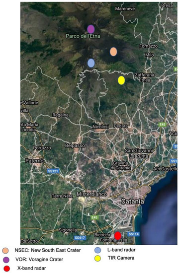
Figure 1.
Map of location of three remote sensing sensors used in this study.
2.1. Thermal Infrared Camera
The thermal-infrared camera is located at ∼15 km (Nicolosi) south from the Etna summit craters and belongs to the video-monitoring network system of the INGV-OE. The TIR camera provides a time series of 640 × 480-pixel images with a spatial resolution of a few meters [22,27] and a thermal sensitivity of 80 mK at 25 °C. The images are displayed with a fixed color scale with a range of −10 to 70 °C. Radiometric data, recorded between 0 and 500 °C, are processed in real-time by a custom written code (i.e., NewSaraterm) [27,28].
The top height of the IJR can be detected by selecting the saturated portion of the measured brightness imagery. The saturation of the camera depends on the properties of the camera and on environmental factors; different thermal surveillance cameras at Etna might, therefore, be saturated in different conditions [20]. Most procedures, used to identify the IJR, are based on setting a suitable threshold to the vertical spatial gradients and/or to edge-contour detection filters. Selecting the TIR camera frames at time intervals of 1 min, it is possible to derive the IJR top height in each image, as described in [20,22,23,25,29].
2.2. The L-Band VOLDORAD-2B Doppler Radar
The VOLDORAD is a fixed-pointing L-band radar (i.e., wavelength of 23.5 cm) that aims at the near-vent detection of erupted material during Etna’s explosive events. This Doppler radar measures both the radial velocity vr and the received backscattered power that characterizes the amount of detected tephra at high time resolution (i.e., 0.2 s). From the observation geometry, it is possible to convert vr into exit velocity vex (i.e., vex = 3.89 vr) [16,17,28], whereas from the specifications of the L-band radar and the radar constant, the backscattered power can be transformed into the L-band reflectivity factor Zhh [15,17].
2.3. The X-Band Polarimetric Weather Radar
The X-band radar is a dual-polarization scanning radar of the Italian weather radar network [30]. This system has the following features: wavelengths of about 3.1 cm (9.6 GHz), transmitted peak power of 50 kW, half-power beam width of 1.3°, and permittivity factor of ash particles (equal to 0.39 with respect to 0.93 of water particles) [12,31]. The X-band radar performs a 3-D scan of the surrounding scene as a function of range, azimuth, and elevation with five azimuthal scans per minutes. The X-band radar acquisitions consist of data volumes having a selected area of about 160 × 160 km2 wide and 20 km height for each considered event. The data volume cross sections are sampled along 12 elevation angles plus a vertical one with a time resolution of 10 min. X-band radar is located at a distance of about 32 km from the NSEC and 33 km from the VOR (see Figure 1).
Generally, microwave weather radars are able to monitor power level variations to determine reflectivity with high accuracy. The calibration of the weather radar equipment is a mandatory procedure with which it is possible to configure the system in a suitable way to carry out quantitative measurements of the reflectivity of a known target. Figure 2 shows the sensitivity of X-band (red line) and L-band (blue line) radars, i.e., the minimum detectable reflectivity (MDZ) for a specified scattering volume at a given distance from radar [12], knowing the operational specifications of both radars. The range of each radar varies according to its specifications. In fact, the L-band radar maximum observable distance is 15 km with a sensitivity ranging from 15 dBZ to 55 dBZ, whereas the X-band radar the maximum observable distance is about 80 km with an MDZ ranging from −58 dBZ to −3 dBZ.
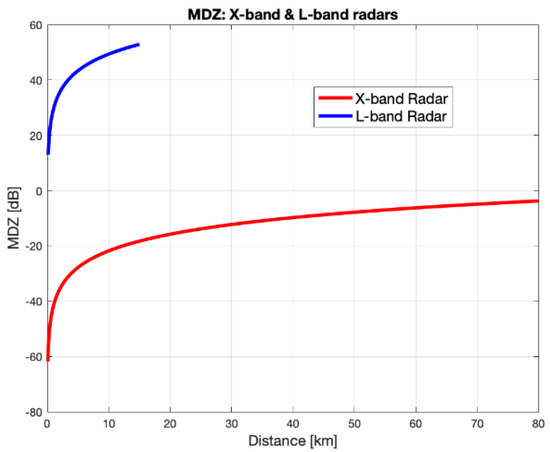
Figure 2.
Minimum detectable signal (MDZ) computed for X-band (red line) and L-band (blue line) radars, known as the operational radar characteristics.
3. Methods
Processing and retrieval methodologies will be illustrated in the following paragraphs for the TIR camera, L-band radar, and X-band radar.
3.1. Thermal-Infrared Camera Algorithms
At Etna, the height of the IJR is identified as the top height of the saturated thermal infrared region, extracted from the thermal-infrared products or images of the TIR camera as shown in Figure 3. The main assumption is that, during lava fountain events, the saturated region of thermal images mainly represents sustained jets of hot tephra and gas [23]. Thermal-infrared camera measurements are hence processed to extract the HIJR from the recorded thermal-infrared brightness temperature imagery TTIR over the eruptive time interval. The TIR camera algorithm is relatively simple and based on a brightness temperature gradient algorithm larger than a given threshold, as tested in [29]. The height of the IJR does not necessarily correspond to the height of the lava fountain because it is mostly associated with the hot region characterized by large clasts. The IJR can also be higher than the lava fountain. Nonetheless, it is worth mentioning that, for simplicity, previous studies have associated the IJR to the lava fountain [22,23,27].
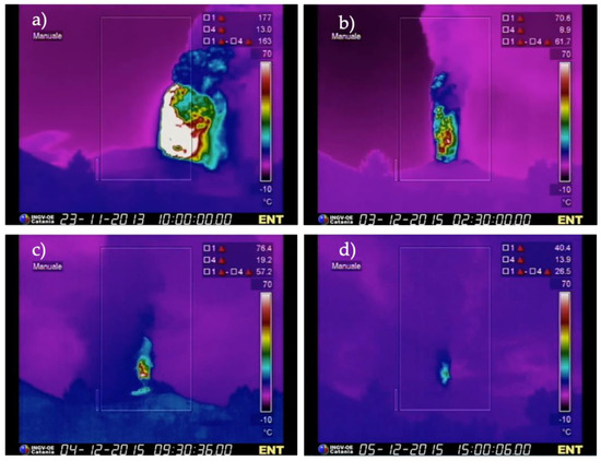
Figure 3.
Frame of the TIR camera in Nicolosi (named ENT) showing the lava fountains from the NSEC for 23 November 2013, panel (a), and from the VOR for 3–5 December 2015 panel (b–d). On the black line below each image, the date (dd-mm-yyyy) and UTC time (hh:mm:ss:00) of the Etna eruptive event are given, respectively.
The IJR height detection from TIR camera images is derived by imposing a thermal infrared condition , i.e., looking for the height above the crater and along the axis z centered on the vent such that the CTIR is satisfied:
where the vertical bar stands for “conditioned to” and (x,y) are the horizontal coordinates. The various conditions are discussed in the next paragraphs. Using a reference target in the TIR camera images with a known position, we can derive a scale factor and convert the TIR image coordinates from pixel numbers to meters. Starting from the time sequence of TIR camera images we can apply the threshold algorithms in order to extract the lava fountain edges, defined by a high temperature change, in each intensity image.
The first TIR condition uses the Canny edge detection [32], looking for local maxima of the TIR temperature gradient, above the vent, by means of the derivative of a Gaussian filter. The Canny method applies two thresholds, shown in Table 1, for the gradient detection: a high threshold tT1 for low-edge sensitivity and a lower threshold tT2 for high-edge sensitivity. Both values are used in order to set the standard deviation of the Gaussian filter. By using two thresholds, the Canny method is less likely than other methods to be fooled by image noise, and more likely to detect true weak edges. In summary, the first TIR condition imposes that the temperature gradient along the vertical axis z is included between tT1 and tT2 as expressed by:
where () indicate the three coordinates (x,y,z) and the time instant t, whereas the curly brackets stand for a set of rules to be satisfied. This TIR camera approach, supported by (2), is hereinafter named TIR Camera-Edge.

Table 1.
Thermal-infrared camera threshold values for the IJR height detection algorithms.
The second TIR condition is obtained by choosing the suitable temperature gradient threshold values tTIR. The HIJR is derived in conditions of good atmospheric visibility as the maximum height of the image saturated region above the vent whose contour is identified by a rapid temperature variation rather than a fixed temperature value, according to the relation:
where tTIR is the TIR camera temperature threshold (see Table 1). This approach, supported by (3), is hereinafter named TIR Camera.
In both previous methods, the IJR height from TIR imagery at a given instant can be extracted as the mean of all hIJR in (1) satisfying the corresponding TIR condition, that is:
where Mean is the average operator over (x,y) coordinates.
3.2. Simulated X-Band Radar Responses
In order to better understand the radar response, we introduce and discuss the main polarimetric radar observables:
- (i).
- The reflectivity factor Zhh, expressed in units of mm6 m−3 or commonly as decibels dBZ. Zhh, is equal within Rayleigh scattering conditions to the integral of the sixth-order moment of the detected particle size distribution, i.e., N(D)D6dD, with N(D) the number distribution (m−3) of particle with diameter D (mm) and size interval dD (mm);
- (ii).
- The differential reflectivity Zdr related to the ratio of reflectivity between the horizontal and vertical polarizations, expressed in dB;
- (iii).
- The copolar correlation coefficient ρhv is a measure of the correlation degree between horizontally and vertically polarized echoes, hence a measure of the variety of particle shapes in a pulse volume between horizontal (H) and vertical (V) polarization radar returns [33].
Starting from the assumptions on the dielectric microphysical model of the tephra particles dispersion, we use the Tephra Particle Ensemble Scattering Simulator (TPESS) for distinguishing tephra orientation, concentration, and typology inside eruptive columns [12,13]. The TPESS simulator is run at X-band frequency for three dimensional tephra classes: coarse ash (CA, particle sizes between 0.063 mm and 2 mm), fine lapilli (FL, particle sizes between 2 mm and 4 mm), and medium lapilli (ML, particle sizes between 4 mm and 16 mm) [34,35] and generated at specific concentration: medium concentration (MC, mass density between 10−1 and 100 g/m3), high or large concentration (LC, mass density between 100 and 101 g/m3) and very high concentration or intense (IC, mass density between 101 and 3∙101 g/m3). The particle average orientations are oblate (red), prolate (blue), and tumbling (green).
In Figure 4, we show the scatterplots of Zhh as a function of ρhv and Zdr. These values are derived from a Monte Carlo generation in the framework of TPESS [13,32,36]. The copolar correlation coefficient shows a response that changes with the increase of particle size and according to the particle orientation (Figure 4). In fact, the largest variations are due to oblate particles, which show a decreasing copolar correlation coefficient as a function of particle size. This superposition, among the particle’s orientation states, makes distinguishing among the three different orientations (oblate, prolate, and tumbling) quite difficult. With increasing particle size, the Zdr signature of the three orientations tends to be merged but they remain distinguishable among each other.
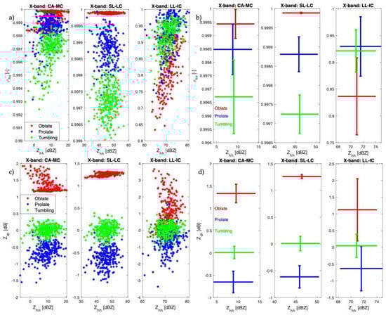
Figure 4.
In panels (a,c) distribution of scatterplots of Zhh (dBZ) as a function of ρhv (adim) and Zdr (dB), respectively, whereas in panels (b,d) the statistic trend of same observables. The intersection of bars represents the mean value and the bar the standard deviation of each radar polarimetric observable, where the different colors refer to particle average orientations: oblate (red), prolate (blue) and tumbling (green).
3.3. Microwave Radar Algorithms
We use the Volcanic Advanced Radar Retrieval (VARR, previously termed as volcanic ash radar retrieval, e.g., [12,13]) to analyze the time series of X-band radar data in order to quantitatively estimate the tephra particle category, mass concentration, MERs and plume height every ten minutes within eruptive columns [13]. The VARR methodology, supported by numerical simulations of plume coupled with lava fountain [10], has been improved in order to consider the strong heterogeneity of the volcanic jet, e.g., composition in microlite, vesicle content, or spindle composition [37].
In contrast with X-band radar and TIR camera that can provide a more direct estimate of HIJR, from L-band radar data we can derive directly the tephra exit velocity vex as a normal projection of the measured radial Doppler velocities [17,25]. However, the latter can be used to retrieve HIJR, based on the Torricelli’s equation [2]. This equation, also deducible from energy conservation, can provide an estimate of HIJR associated with the vertically directed outflow velocity vex of a constant jet from the eruptive vent, and vice-versa. Indeed, the Torricellli equation is a valid approximation when most of the pyroclasts are sufficiently large to be considered as being uniformly accelerated projectiles that do not enter into the upper convective region of the plume [2,25] as well as atmospheric density variations and drag effects are negligible. Under these assumptions, at each timestep t using for the L-band fixed-pointing radar we can write:
where g (m/s2) is the Earth gravity acceleration and the superscript L stands for L-band radar.
The multisensor approach to IJR height detection and retrieval aims at:
- (1)
- Exploring X-band radar data potential to detect and estimate the height of the IJR from its polarimetric signatures.
- (2)
- Integrating X-band radar estimates with the IJR height retrievals from L-band estimates used as a constraint.
- (3)
- Comparing X-band radar and TIR camera observations in order to better understand the link between the IJR and the lava fountains and to reduce errors in their respective IJR height estimates.
Physically speaking, we can consider the IJR area as a turbulent volume above the crater in which the gas represents the driving component of the pyroclastic jet. In this region, based on the polarimetric X-band synthetic signatures discussed in the previous Section 3.2, the copolar correlation coefficient should show lower values at lower altitudes within the jet region and tends to increase as the turbulent motion decreases. At the same time, the reflectivity factor should reach quite high values (say, greater than 45 dBZ at X band), related to the increase in the heterogeneity of tephra coarse particles being pushed out of the crater at high speed. From Figure 4, in particular, we should expect a significant decrease of Zhh near the top of the IJR due to the decrease of the average particle size in the plume-fed by lava fountain, as well as a decrease of ρhv due to the predominant tumbling effect and turbulence within the eruption column. This behavior is typical of the transition zone between the lava fountains and the convective zone of volcanic plumes [2]. Moreover, near the top of IJR, the Zdr values tend to increase due to larger non-spherical particles and reduced turbulence inducing less tumbling above the lava fountain. This is the physical rationale of the incandescent jet region radar retrieval algorithm (JR3A) approach, based on the analysis of the vertical gradients of polarimetric observables Zhh and ρhv as well as L-band estimates if available.
The JR3A methodology is a decision approach for detecting HJIR, based on the following steps:
(i) Select an area AWR = (Δx, Δy) within the Cartesian horizontal coordinates x and y (derived from the radar projected azimuth and range coordinates at the lowest elevation), centered on volcanic vent expected position and define a volume VWR = (AWR, Δz) = (Δx,Δy,Δz) where vertical interval Δz above the vent extends preliminarily up to the expected maximum IJR height. In this work (Δx, Δy) are set to less than 3 km and Δz is set equal to 3 km (an IJR higher than 3 kilometers is improbable).
(ii) Calculate the mean value and standard deviation of Zhh and ρhv within the selected volume VWR and compute the standardized values of and , centered with respect to respective mean values and divided with respect to standard deviation of Zhh and ρhv. Then select within the volume VWR, the incandescent jet-region sub-volume VIJR verifying a combined polarimetric condition , i.e., both (x,y,t) lower than tz and (x,y,t). lower than tρ, that is similarly to (2) and (3):
where the polarimetric thresholds values, used in this work for the X-band radar, are tz = 2 and tρ = 1 (both adimensional).
(iii) Compute the vertical gradient ∇ along z for each column (x∈Δx, y∈Δy) within the volume VWR at each time step (depending on the scanning radar sampling time) of the reflectivity factor, named (x,y,t), and of the copolar correlation coefficient, named (x,y,t).
(iv) Search for the IJR heights above the crater and along the vertical coordinate axis z, such that previous conditions in (6) are satisfied on X-band radar reflectivity and copolar correlation coefficient, where the superscript X stands for X-band radar.
(v) Apply the Torricelli equation in (5) to the exit velocity vex normal to the crater surface, derived from the L-band radar measurements, to estimate the IJR height ;
(vi) Select the set heights corresponding and different to zero within the X-band radar volume, minimizing the difference between , derived from L-band radar velocities measurements ([25,38]), and each height of X-band radar volumes, that is we can write:
where Min is the minimization operator over (x,y) and WR stands for X-band weather radar. If L-band radar data are not available, this step can be skipped.
(vii) Compute the maximum height within all estimates in (7) and add the uncertainty ΔhHPBW representing the half-opening of the radar beam with respect to its boresight, namely at each time step we can obtain:
where Max is the maximum operator over (x,y). It should be noted that is the altitude above the summit crater (in the Etna case, about 3 km above sea level), whereas the half cross-section ΔhHPBW of the radar main-beam along the vertical above the crater is range dependent (in our case, around 300 m [25]).
4. Etna Case Studies
The recent paroxysmal activity at Etna was characterized by more than 150 lava fountain-fed tephra plume events lasting from 20 min up to several hours. Typically, these ash-rich events generate sustained plumes whose heights often exceed 10 km above sea level (a.s.l.) and usually impact the local population and air traffic [19,39,40,41]. Here, we analyzed 5 paroxysmal episodes that occurred between 2013 and 2015.
4.1. Paroxysm of 23 November 2013
On 23 November 2013 a lava fountain produced an intense explosive activity from the NSEC (Figure 5) for about an hour. Previous studies on this event focused on the eruptive processes and tephra volumes [22], integration of observational data [41], tephra fallout characterization [42], plume dynamics [43] and total grain-size distribution retrievals [25,44]. Figure 5 shows the range-height distribution of reflectivity factor, copolar correlation coefficient and differential reflectivity. Looking at these measurements, close to the NSEC, we notice a column showing increasing Zhh values (pixels in red/orange) above the crater and decreasing values of ρhv (pixels in green/blue). A similar trend is shown in the Zhh and Zdr signatures. For the 23 November 2013 eruption, shown in Figure 5, the lowest values of ρhv are observed only in the lateral parts of the first portion of the eruptive column. As observed by [43], ρhv displays a notably low signature above the crater during the violent phase of the explosive activity corresponding to what we call the IJR.
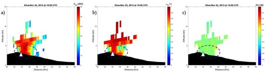
Figure 5.
X-Band radar retrieval of Etna explosive activity of 23 Nov. 2013 at 10:00 UTC. Range-Height Indicator (RHI) of the reflectivity factor Zhh (dBZ) in panel (a), copolar correlation coefficient ρhv (admin) in panel (b) and in (c) Zdr (dB) of X-band radar along the radar azimuth intercepting the volcanic vent. The white triangle identifies the position of the NSEC.
4.2. Paroxysms on 3–5 December 2015
Starting in the second half of October 2015, the VOR produced an intra-crater Strombolian activity that progressively increased and culminated in four lava fountains on 3, 4 and 5 December. These episodes, each lasting 50–60 min, generated eruptive columns reaching 15 km asl [45]. Figure 6 shows the RHI (from left to right) of the range-height distribution of reflectivity factor, copolar correlation coefficient and differential reflectivity for those events on 3 December 2015 at 02:30 UTC (a), on 4 December 2015 at 09:30 UTC (b), 4 December 2015 at 21:00 UTC (c) and on 5 December 2015 at 15:00 UTC (d). In the case of the 2015 events, the different polarimetric responses of the IJR are also visible in the RHI patterns. In particular, the lava fountain and the eruption column are well detectable since, corresponding to high Zhh value near the crater, moderate values of ρhv and a high Zdr are observed for each event.
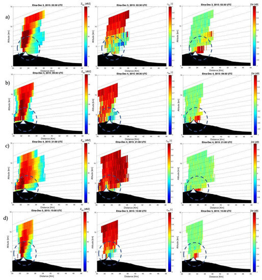
Figure 6.
X-Band radar retrievals of Etna explosive activity on 3 December 2015 at 02:30 UTC (a), on 4 December 2015 at 09:30 UTC (b), 4 December 2015 at 21:00 UTC and (c) on 5 December 2015 at 15:00 UTC (d). Range-Height Indicator (RHI) of the reflectivity factor Zhh (dBZ), copolar correlation coefficient ρhv (admin) and Zdr (dB) of X-band radar along the radar azimuth intercepting the vent. The white triangle identifies the position of the NSEC and VOR craters.
5. Results
In this section, we will demonstrate the potential of using X-band polarimetric radar observables, such as ρhv jointly with Zhh, together with L-band radar constraints, to detect and estimate the IJR height. As anticipated, we will compare radar-based retrievals of IJR height with the estimates extracted from the TIR camera.
The left panels of Figure 7 (related to 23 November 2013 paroxysm) and Figure 8 (related to 3, 4, and 5 December 2015 events) show the horizontally averaged vertical profile at a certain time of Zhh and ρhv at the instant of maximum X-band radar HJIR estimates (above the vent). The vertical profile of ρhv gradually increases with altitude, whereas the Zhh profiles initially increase at middle altitude and then decrease as they reach the plume top height. The drop of ρhv in the far side of the column is likely related to a low signal-to-noise ratio (SNR), as it corresponds to low reflectivity values [46]. A general increase in the copolar correlation coefficient with increasing altitudes can be due to a reduction of turbulent motion. Interestingly, the lowest value of ρhv coincides with the top of the IJR. Based on radar signatures shown in Figure 4, the IJR internal patterns of Zhh and ρhv are associated with the behavior of a jet dominated by ballistic blocks, bombs, and lapilli. Moreover, these signatures could be related to the relative amplification of particle heterogeneity due to the reduction of size sorting depending on the vertical velocity [30]. The continuous lines in the left panels of Figure 7 and Figure 8 identify the HIJR (as the center height of the radar beam) in function of time (as indicated in the title of each panel). The dashed lines represent the two edges of the main-beam aperture at the same height, i.e., the uncertainty of the HIJR estimates.
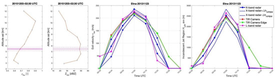
Figure 7.
On the left: horizontally averaged vertical profile at the specific time of the copolar correlation coefficient ρhv (adim) and the reflectivity factor Zhh (dBZ) during the explosive activity on 23 November 2013 at 10:10 UTC. The brown line identifies the mean value, whereas the small horizontal blue bars correspond to the standard deviations computed at each altitude related to radar elevation angles above the vent. The magenta line identifies the altitude where the algorithm, at the specified time, simultaneously maximizes Zhh and minimizes as much as possible ρhv, whereas the two dashed magenta lines quantify the altitude variability range. In the middle and on the right panels, we show the time-series having a time step of 10 min of vex and HIJR respectively. The HIJR is directly extracted from two TIR camera approaches, TIR Camera and TIR Camera-Edge, and the L-band and X-band radar, latter expressed as in function of the uncertainty ΔhHPBW (about 300 m) correlated to half-power beam width of X-band radar.
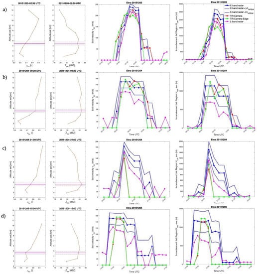
Figure 8.
Horizontally averaged vertical profile at the specific time of the copolar correlation coefficient ρhv (adim) and the reflectivity factor Zhh (dBZ) during the explosive activity on 3 December 2015 at 02:30 UTC (a), 4 December 2015 at 09:30 UTC (b) and at 21:00 UTC (c) and 5 December 2015 at 15:00 UTC (d), respectively. The brown line identifies the mean value, whereas the small horizontal blue bars identify the standard deviations computed at each altitude related to radar elevation angles above the crater. Two dashed magenta lines identify the altitude variability range where the algorithm searches at the specified time to maximize Zhh and minimize ρhv. In the middle and on the right panels, we show the time-series having a time step of 10 min of vex and HIJR respectively. The HIJR is directly extracted from two TIR camera approaches, TIR Camera and TIR Camera-Edge as in (2) and (3) respectively, and the L-band and X-band radar, latter expressed as in function of the uncertainty ΔhHPBW (about 300 m) related to half-power beam width of X-band radar.
The central and right-hand panels of Figure 7 and Figure 8, panels a–d, show the comparisons among the time-series of vex and HIJR, derived respectively from the TIR camera (TIR Camera and TIR Camera-Edge), X-band and L-band radar. In detail, the central panel of Figure 7 shows an increasing trend of vex with a maximum value of 215–225 m/s at 10:00 UTC. In the left-hand panel, a similar increasing trend of TIR camera-derived HIJR starting from 9:30 UTC is observed with a peak of 2500 m at 10:00 UTC, using the TIR Camera algorithm as expressed in (2), then decreasing to a few meters at 10:30 UTC, and a peak of 2460 m, using the TIR Camera algorithm as expressed in (3), at 10:00 UTC, decreasing similarly to previous estimation. The X-band radar observes HIJR only from 09:30–10:20 UTC with a final estimate between 10:00 UTC of 2530 m above the vent. An uncertainty ΔhHPBW (about 300 m) is associated to X-band radar retrievals and expressed as a function of half power beam width. Accordingly, this uncertainty is plotted in each panel as dashed lines indicated by HIJR +/− ΔhHPBW. The height peaks observed by each sensor method show a very similar value of 2500 m. This minimal difference among retrievals is probably due to the X-band radar sensitivity to the microphysical characteristics of the detected particle, according to the combination of radar observables.
In the panel (a) of the central part of Figure 8, each vex values range between 200 and 250 m/s from 02:00 to 03:20 UTC, highlighting a good agreement among values obtained by all methods, with the greatest value detected by the X-band radar and lowest by the L-band radar; in (b) the variability of vex detected by the X-band radar incorporates the TIR camera values from 09:00 until 10:10 UTC with values ranging between 130 and 170 m/s, whereas the L-band velocities show the lowest values; in (c) all retrievals indicate a peak value of 140–200 m/s at the same time, i.e., 20:40 UTC. In this case, the time range detected by TIR camera is limited to 20:30 until 20:50 UTC; in (d) Similarly, the variability of vex detected by the X-band radar incorporates the TIR camera values between 09:00 and 10:10 UTC, whereas the L-band shows the lowest values that range between 130 and 170 m/s from 14:20 to 15:10 UTC.
In the panel (a) on the right of Figure 8 there is a longer temporal extension of the HIJR from the TIR camera (01:30 and 03:30 UTC), while for the radar the IJR-detected interval is between 01:50–03:50 UTC. The maximum of IJR height is obtained by X-band radar estimates at 02:30 UTC, with a value of 2900 m ± 300 m (ΔhHPBW) and two TIR camera peaks of 2250 m at 02:20 and of 2600 m at 02:40 UTC. In the right panel (b) a temporal agreement is observed in the identification of heights among the various methods between 09:00 and 10:30 UTC. The peaks for the TIR camera are at 09:20 UTC with a value around 1300 m. The X-band radar estimate presents a constant value of 1150 m ± 300 m (ΔhHPBW) between 09:10 and 09:30 UTC. On the evening of 4 December 2015, right panel (c) the TIR camera estimates are limited to a small interval between 20:20 and 20:50 UTC with a peak at 20:40 UTC of about 1000 m and 1150 m. The X-band radar estimates, instead, present a longer time interval going from 20:10 to 21:40 UTC with a peak of 1700 m ± 300 m (ΔhHPBW) at 20:40 UTC. Similarly to the previous case, on 5 December 2015 (right panel (d)), the incandescent region height estimates from TIR camera show a consistent estimate only between 14:20 and 15:10 UTC, probably for the poor visibility due to weather clouds and an HIJR value of 1150 m and 1250 m.
The X-band radar, thanks to its scanning capacity in elevation and azimuth and little sensitivity to small water droplets of non-precipitating clouds, provides an estimate of HIJR within the interval between 14:10 UTC to 16:30 UTC. Its estimated height between 14:10 UTC and 15:10 UTC is quite constant (about 1200 m ± 300 m (ΔhHPBW)) and with a secondary peak of 200 m at 16:20 UTC. It should be noted that a temperature drop detected by the TIR camera of about ten degrees has been observed, correlated to some meteorological phenomenon, as confirmed by the video cameras of INGV-OE, that is interposed between the TIR camera and the eruptive plume with consequent lowering of the HIJR identification thresholds. Observing the various HIJR retrievals from the X-band radar compared to those obtained from the TIC camera, it emerges that the radar can detect the IJR observed by the camera. If we take into account the discretization of the altitudes detected by the X-band radar, due to the observation angle and the distance between the radar and the volcanic plume, and given its uncertainty relative to the ΔhHPBW, the HIJR estimates of the X-band radar are quite similar to the TIR camera estimates.
The lower estimates of the TIR camera, especially between 20:00 and 22:00 UTC on 4 December and during the 5 December 2015 events (Figure 8c,d) are mainly due to bad weather conditions. Indeed, the presence of meteorological water clouds in Etna’s summit area results in a strong degradation of the detected brightness temperature. For this reason, the detected heights are limited to narrow time intervals with respect to what was detected by the two radars. This variation is less evident when comparing both X-band radar and L-band radar estimates, although the X-band radar polarimetric signatures appear significantly cleaner in November 2013, due to the absence of any meteorological phenomenon at the same time as the eruption, than in December 2015 (see Figure 7 and Figure 8), as well as for a different resolution of the radar beam.
In addition, we quantified the vertical gradient variability of reflectivity factor and copolar correlation coefficient involved in the HIJR determination (panel a) in the Figure 9a). The values of ∇Zhh follow the range (7.20 dBZ +/− 8.50 dBZ), whereas the values of ∇ρhv are in within (−0.06 +/− 0.16). In Figure 9b, the bars of vertical gradient of reflectivity factor and copolar correlation coefficient, related to five events, are plotted in different colors. Moreover, to quantify the difference in the IJR height estimates with the two sensors, we compute the difference between the retrievals , derived from X-band radar using (8), and from TIR camera using (4) (TIR Camera algorithm), as expressed below:
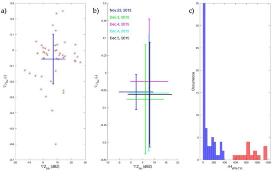
Figure 9.
Panel (a) shows the scatterplot of the reflectivity factor vertical gradient ∇Zhh and copolar correlation coefficient vertical gradient ∇ρhv for all analyzed events with the horizontal and vertical bars delimiting the dispersion of gradients. In panel (b) the dispersion bar of ∇Zhh and ∇ρhv related to five eruptive events are plotted in different colors, whereas panel (c) is the histogram of difference between the HIJR derived from X-band radar and the TIR camera for both Etna events. Red bars refer in panel (c) to the cases where TIR camera is obscured by clouds.
The few higher values, shown in the tail of the histogram, ranging between 590 m and 1180 m and with mean value of 890 m, are related to the limited operativity of the TIR camera instrument for lava fountain detection due to the occurrence of meteorological clouds, as described before (Figure 9c). The X-band radar generally guarantees a “microwave” visibility of both plume and lava fountain activity in the cases of limited view conditions as during an explosive activity, thanks to the very good receiver sensitivity and effective penetration into volcanic jets and plumes.
The comparison of the results, obtained for the event of 23 November 2013 and 3–5 December 2015, shows a promising agreement. Our comparative analyses of the polarimetric radar measurements provides estimates of the IJR heights. Here, we might validate the use of such heights to retrieve first order estimates of MER during paroxysms at Etna [20,25,30]. Indeed, MER can be derived using the area of the eruptive vent, the magma-gas mixture density and the exit velocity (surface flux approach in [25]). If we consider the IJR height as a proxy for the height of the lava fountain [22,23,27], it can then be related to an exit velocity vex through the well-known Torricelli equation for a non-viscous ballistic flow [25,26,27]. When making this assumption, it is, however, important to bear in mind that the IJR can be higher than the lava fountains due to hot blocks, bombs, and lapilli that reach higher levels or lower levels when covered by volcanic ash.
Assuming that lava fountains feed the associated tephra plumes, the retrieved MER can be used to estimate the total mass of tephra emitted during a paroxysmal episode at Etna. Part of them will build the scoria cone [28,47] while the finest particles will feed the eruption column.
6. Conclusions
Describing lava fountain-fed tephra plumes and quantifying their dynamics is crucial to monitoring and hazard assessment but it is by no means trivial. The thermal-infrared camera provides 2D information on the near-source environment of the eruptive columns at Etna. However, the internal structure of the eruption column cannot be investigated, and thermal images suffer from severe degradation when meteorological clouds are present. The L-band radar with fixed pointing on the eruptive crater can only scan the first portion of the plume. On the contrary, X-band radar can scan the entire eruptive column in 3D volumes, providing accurate information of its geometrical and microphysical parameters with less weather restrictions. In this study, we also confirm the capacity of X-band radar to investigate the lava fountains and tephra plume activity during explosive eruptions.
Our analyses have shown how the patterns of the polarimetric observables Zhh and ρhv, as detected from the X-band radar, provide a good estimate of the IJR height when compared to those obtained from the TIR camera. The radar signature of IJR is compatible with a jet of blocks, bombs, and lapilli. As previously discussed, the IJR can be of different height with respect to the lava fountain due to hot blocks, bombs and lapilli that reach higher levels or lower levels when covered by volcanic ash. Nonetheless, for the sake of simplicity, and in agreement with previous studies [22,23,27], the height of IJR has been used as a proxy for the height of the lava fountain in order to derive the exit velocity of the mixture. The exit velocity of the mixture can then be used to determine the associated MER and total erupted mass. In any case, it is important to also stress that the IJR and the lava fountain cannot be considered as a proxy of the gas thrust region of the associated plume [10].
In this work, we have demonstrated the importance of the combined use of TIR camera, X-band polarimetric and L-band Doppler radars for the characterization of paroxysmal activity at Etna. Further quantitative information should be obtained from multi-sensor strategies to investigate the link between lava fountains and IJR at other volcanoes and or eruptive events.
Author Contributions
Conceptualization, L.M. and F.S.M.; methodology, L.M. and F.S.M.; software, L.M.; validation, L.M.; formal analysis, L.M. and F.S.M.; investigation, L.M., S.S., C.B., V.F.-L., and F.S.M.; resources, L.M.; data curation, L.M.; writing—original draft preparation, L.M.; writing—review and editing, F.SM., S.S., C.B., and V.F.-L.; visualization, L.M.; supervision, F.S.M. and S.S.; project administration, F.S.M. and C.B.; funding acquisition, C.B. All authors have read and agreed to the published version of the manuscript.
Funding
This project has received funding from the European Union’s Horizon 2020 research and innovation programme under grant agreement No 731070 (EUROVOLC).
Acknowledgments
The Thermal Infrared Camera on Etna is operated with INGV-OE and we thank all technicians of INGV-OE who are involved in the maintenance of the camera. We also thank F. Donnadieu of CNRS, IRD, OPDG of Université of Clermont Auvergne for the VOLDORAD data and the Italian Department of Civil Protection (DPC, Italy) for providing the X-band radar. VOLDORAD 2B is operated jointly by the OPGC and INGV-OE (Catania, Italy) in the framework of a collaboration agreement between INGV-OE, the French CNRS, and the OPGC-Université Clermont Auvergne in Clermont-Ferrand (France). Stephen Conway, an English native mother speaker for INGV-OE is also thanked.
Conflicts of Interest
The authors declare no conflict of interest.
References
- Du Preez, D.V.; Bencherif, H.; Bègue, N.; Clarisse, L.; Hoffman, R.F.; Wright, C.Y. Investigating the Large-Scale Transport of a Volcanic Plume and the Impact on a Secondary Site. Atmosphere 2020, 11, 548. [Google Scholar] [CrossRef]
- Sparks, R.S.J. The dimensions and dynamics of volcanic eruption columns. Bull. Volcanol. 1986, 48, 3–15. [Google Scholar] [CrossRef]
- Woodhouse, M.J.; Hogg, A.J.; Phillips, J.C. A global sensitivity analysis of the PlumeRise model of volcanic plumes. J. Volcanol. Geotherm. Res. 2016, 326, 54–76. [Google Scholar] [CrossRef]
- Self, S. The effects and consequences of very large explosive volcanic eruptions. Philos. Trans. R. Soc. A Math. Phys. Eng. Sci. 2006, 364, 2073–2097. [Google Scholar] [CrossRef] [PubMed]
- Carazzo, G.; Kaminski, E.; Tait, S. On the dynamics of volcanic columns: A comparison of field data with a new model of negatively buoyant jets. J. Volcanol. Geotherm. Res. 2008, 178, 94–103. [Google Scholar] [CrossRef]
- Suzuki, Y.J.; Koyaguchi, T. A three-dimensional numerical simulation of spreading umbrella clouds. J. Geophys. Res. 2009, 114, B03209. [Google Scholar] [CrossRef]
- Esposti Ongaro, T.; Clarke, A.B.; Neri, A.; Voight, B.; Widiwijayanti, C. Fluid dynamics of the 1997 Boxing Day volcanic blast on Montserrat, West Indies. J. Geophys. Res. 1995, 113, B03211. [Google Scholar] [CrossRef]
- Wilson, L.; Parfitt, E.A.; Head, J.W. Explosive volcanic eruptions—VIII. The role of magma recycling in controlling the behaviour of Hawaiian-style lava fountains. Geophys. J. Int. 1995, 121, 215–225. [Google Scholar] [CrossRef]
- Taddeucci, J.; Edmonds, M.; Houghton, B.; James, M.R.; Vergniolle, S. Hawaiian and Strombolian Eruptions. The Encyclopedia of Volcanoes; Elsevier Inc.: Amsterdam, The Netherland; University of Rhode Island: Narragansett, RI, USA, 2015; pp. 485–503. [Google Scholar]
- Snee, E.; Degruyter, W.; Bonadonna, C.; Scollo, S.; Rossi, E.; Freret-Lorgeril, V. A model for buoyant tephra plumes coupled to lava fountains with an application to paroxysmal eruptions at Mount Etna. JGR Solid Earth 2020. submitted. [Google Scholar]
- Bonadonna, C.; Folch, A.; Loughlin, S.; Puempel, H. Future developments in modelling and monitoring of volcanic ash clouds: Outcomes from the first IAVCEI-WMO workshop on Ash Dispersal Forecast and Civil Aviation. Short Sci. Commun. Bull. Volcanol. 2011, 74, 1–10. [Google Scholar] [CrossRef]
- Marzano, F.S.; Picciotti, E.; Vulpiani, G.; Montopoli, M. Synthetic signatures of volcanic ash cloud particles from X-band dual-polarization radar. IEEE Trans. Geosci. Remote Sens. 2012, 50, 193–211. [Google Scholar] [CrossRef]
- Mereu, L.; Marzano, F.S.; Montopoli, M.; Bonadonna, C. Retrieval of tephra size spectra and mass flow rate from C-Band radar during the 2010 Eyjafjallajökull eruption, Iceland. IEEE Trans. Geosci. Remote Sens. 2015, 3, 5644–5660. [Google Scholar] [CrossRef]
- Scollo, S.; Prestifilippo, M.; Bonadonna, C.; Cioni, R.; Corradini, S.; Degruyter, W.; Rossi, E.; Silvestri, M.; Biale, E.; Carparelli, G. Near-Real-Time Tephra Fallout Assessment at Mt. Etna, Italy. Remote Sens. 2019, 11, 2987. [Google Scholar] [CrossRef]
- Ripepe, M.; Bonadonna, C.; Folch, A.; Delle Donne, D.; Lacanna, G.; Marchetti, E.; Hoskuldsson, A. Ash-plume dynamics and eruption source parameters by infrasound and thermal imagery: The 2010 Eyjafjallajokull eruption. Earth Planet. Sci. Lett. 2013, 366, 112–121. [Google Scholar] [CrossRef]
- Donnadieu, F. Volcanological applications of Doppler radars: A review and examples from a transportable pulse radar in L-band. In Doppler Radar Observations-Weather Radar, Wind Profiler, Ionospheric Radar, and Other Advanced Applications; Bech, J., Chau, J.L., Eds.; InTech: London, UK, 2012; pp. 409–446. ISBN 978-953-51-0496-4. [Google Scholar]
- Freret-Lorgeril, V.; Donnadieu, F.; Scollo, S.; Provost, A.; Fréville, P.; Guéhenneux, Y.; Hervier, C.; Prestifilippo, M.; Coltelli, M. Mass eruption rates of tephra plumes during the 2011–2015 lava fountain paroxysms at Mt. Etna from Doppler radar retrievals. Front. Earth Sci. 2018, 6. [Google Scholar] [CrossRef]
- Marzano, F.S.; Barbieri, S.; Vulpiani, G.; Rose, I.W. Volcanic Ash Cloud Retrieval by Ground-Based Microwave Weather Radar. IEEE Trans. Geosci. Remote Sens. 2006, 44, 11. [Google Scholar] [CrossRef]
- Scollo, S.; Prestifilippo, M.; Spata, G.; D’Agostino, M.; Coltelli, M. Monitoring and forecasting Etna volcanic plume. Nat. Hazards Earth Syst. Sci. 2009, 9, 1573–1585. [Google Scholar] [CrossRef]
- Calvari, S.; Cannavò, F.; Bonaccorso, A.; Spampinato, L.; Pellegrino, A.G. Paroxysmal Explosions, Lava Fountains and Ash plumes at Etna Volcano: Eruptive Processes and Hazard Implications. Front. Earth Sci. 2018, 6, 107. [Google Scholar] [CrossRef]
- Corradini, S.; Montopoli, M.; Guerrieri, L.; Ricci, M.; Scollo, S.; Merucci, L.; Marzano, F.S.; Pugnaghi, S.; Prestifilippo, M.; Ventress, L.; et al. A multi-sensor approach for the volcanic ash cloud retrievals and eruption characterization. Remote Sens. 2016, 8, 58. [Google Scholar] [CrossRef]
- Bonaccorso, A.; Calvari, S.; Linde, A.; Sacks, S. Eruptive processes leading to the most explosive lava fountain at Etna volcano: The 23 November 2013 episode. Geophys. Res. Lett. 2014, 41, 4912–4919. [Google Scholar] [CrossRef]
- Carbone, D.; Zuccarello, L.; Messina, A.; Scollo, S.; Rymer, H. Balancing bulk gas accumulation and gas output before and during lava fountaining episodes at Mt. Etna. Nat. Sci. Rep. 2015. [Google Scholar] [CrossRef]
- Sciotto, M.; Cannata, A.; Prestifilippo, M.; Scollo, S.; Fee, D.; Privitera, E. Unravelling the links between seismo-acoustic signals and eruptive parameters: Etna lava fountain case study. Nature 2019, 9, 16417. [Google Scholar] [CrossRef] [PubMed]
- Marzano, F.S.; Mereu, L.; Scollo, S.; Donnadieu, F.; Bonadonna, C. Tephra Mass Eruption Rate from Ground-Based X-Band and L-Band Microwave Radars During the November 23, 2013, Etna Paroxysm. IEEE Trans. Geosci. Remote Sens. 2019, 58, 3314–3327. [Google Scholar] [CrossRef]
- Sparks, R.S.J.; Bursik, M.I.; Carey, S.N.; Gilbert, J.S.; Glaze, L.S.; Sigurdsson, H.; Woods, A.W. Volcanic Plumes; John Wiley & Sons: West Sussex, UK, 1997; 574p. [Google Scholar]
- Calvari, S.; Salerno, G.G.; Spampinato, L.; Gouhier, M.; La Spina, A.; Pecora, E.; Harris, A.J.L.; Labazuy, P.; Biale, E.; Boschi, E. An unloading foam model to constrain Etna’s 11–13 January 2011 lava fountaining episode. J. Geophys. Res. 2011, 116, B11207. [Google Scholar] [CrossRef]
- Behncke, B.; Falsaperla, S.; Pecora, E. Complex magma dynamics at Mount Etna revealed by seismic, thermal and volcanological data. J. Geophys. Res. Atmos. 2009. [Google Scholar] [CrossRef]
- Delle Donne, D.; Ripepe, M. High-frame rate thermal imagery of Strombolian explosions: Implications for explosive and infrasonic source dynamics. J. Geophys. Res. 2012, 117, B09206. [Google Scholar] [CrossRef]
- Vulpiani, G.; Ripepe, M.; Valade, S. Mass discharge rate retrieval combining weather radar and thermal camera observations. J. Geophys. Res. Solid Earth 2016, 121, 5679–5695. [Google Scholar] [CrossRef]
- Montopoli, M.; Vulpiani, G.; Cimini, D.; Picciotti, E.; Marzano, F.S. Interpretation of observed microwave signatures from ground dual polarization radar and space multi-frequency radiometer for the 2011 Grimsvotn volcanic eruption. Atmos. Meas. Tech. 2014, 7, 537–552. [Google Scholar] [CrossRef]
- Canny, J. A Computational Approach to Edge Detection. IEEE Trans. Pattern Anal. Mach. Intell. 1986, PAMI-8, 679–698. [Google Scholar] [CrossRef]
- Mereu, L.; Scollo, S.; Mori, S.; Boselli, A.; Leto, G.; Marzano, F.S. Maximum-Likelihood Retrieval of Volcanic Ash Concentration and Particle Size from Ground-Based Scanning Lidar. IEEE Trans. Geosci. Remote Sens. 2018, 56, 5824–5842. [Google Scholar] [CrossRef]
- Fisher, R.V.; Schmincke, H.-U. Pyroclastic Rocks; Springer: New York, NY, USA, 1984; 472p. [Google Scholar]
- White, J.D.L.; Houghton, B.F. Primary volcaniclastic rocks. Geology 2006, 34, 677–680. [Google Scholar] [CrossRef]
- Mishchenko, M.I. Calculation of the amplitude matrix for a nonspherical particle in a fixed orientation. Appl. Opt. 2001, 39, 1026–1031. [Google Scholar] [CrossRef] [PubMed]
- Hamilton, C.W.; Fitch, E.P.; Fagents, S.A.; Thordarson, T. Rootless tephra stratigraphy and emplacement processes. Bull Volcanol. 2017, 79, 11. [Google Scholar] [CrossRef]
- Donnadieu, F.; Freville, P.; Hervier, C.; Coltelli, M.; Scollo, S.; Prestifilippo, M.; Valade, S.; Rivet, S.; Cacault, P. Near-source Doppler radar monitoring of tephra plumes at Etna. J. Volcanol. Geotherm. Res. 2016, 312, 26–39. [Google Scholar] [CrossRef]
- Ulivieri, G.; Ripepe, M.; Marchetti, E. Infrasound reveals transition to oscillatory discharge regime during lava fountaining: Implication for early warning. Geophys. Res. Lett. 2013, 40, 3008–3013. [Google Scholar] [CrossRef]
- Scollo, S.; Prestifilippo, M.; Pecora, E.; Corradini, S.; Merucci, L.; Spata, G.; Coltelli, M. Eruption column height estimation of the 2011–2013 Etna lava fountains. Ann. Geophys. 2014, 57, S0214. [Google Scholar] [CrossRef]
- Coltelli, M.; Miraglia, L.; Scollo, S. Characterization of shape and 816 terminal velocity of tephra particles erupted during the 2002 eruption 817 of Etna volcano, Italy. Bull. Volcanol. 2008, 70, 1103–1112. [Google Scholar] [CrossRef]
- Andronico, D.; Scollo, S.; Cristaldi, A. Unexpected hazards from tephra fallouts at Mt Etna: The 23 November 2013 lava fountain. J. Volcanol. Geotherm. Res. 2015, 304, 118–125. [Google Scholar] [CrossRef]
- Montopoli, M. Velocity profiles inside volcanic clouds from three- dimensional scanning microwave dual-polarization Doppler radars. J. Geophys. Res. Atmos. 2016, 121, 7881–7900. [Google Scholar] [CrossRef]
- Poret, M.; Corradini, S.; Merucci, L.; Costa, A.; Andronico, A.; Montopoli, M.; Vulpiani, G.; Freret-Lorgeril, V. Reconstructing volcanic plume evolution integrating satellite and ground-based data: Application to the 23rd November 2013 Etna eruption. Atmos. Chem. Phys. Discuss. 2017. [Google Scholar] [CrossRef]
- Pompilio, M.; Bertagnini, A.; Del Carlo, P.; Di Roberto, A. Magma dynamics within a basaltic conduit revealed by textural and compositional features of erupted ash: The December 2015 Mt. Etna Paroxysms. Sci. Rep. 2017, 7, 4805. [Google Scholar] [CrossRef] [PubMed]
- Bringi, V.N.; Chandrasekar, V. Polarimetric Doppler Weather Radar; Cambridge University Press: Cambridge, UK, 2011; p. 636. [Google Scholar]
- De Beni, E.B.; Behncke, S.; Branca, I.; Nicolosi, R.; Carluccio, F.; D’Ajello, C.; Chiappini, M. The continuing story of Etna’s New Southeast Crater (2012–2014): Evolution and volume calculations based on field surveys and aerophotogrammetry. J. Volcanol. Geotherm. Res. 2015, 303, 175–186. [Google Scholar] [CrossRef]


Publisher’s Note: MDPI stays neutral with regard to jurisdictional claims in published maps and institutional affiliations. |
© 2020 by the authors. Licensee MDPI, Basel, Switzerland. This article is an open access article distributed under the terms and conditions of the Creative Commons Attribution (CC BY) license (http://creativecommons.org/licenses/by/4.0/).