Flood Mapping in Vegetated Areas Using an Unsupervised Clustering Approach on Sentinel-1 and -2 Imagery


Abstract
:
1. Introduction
2. Materials
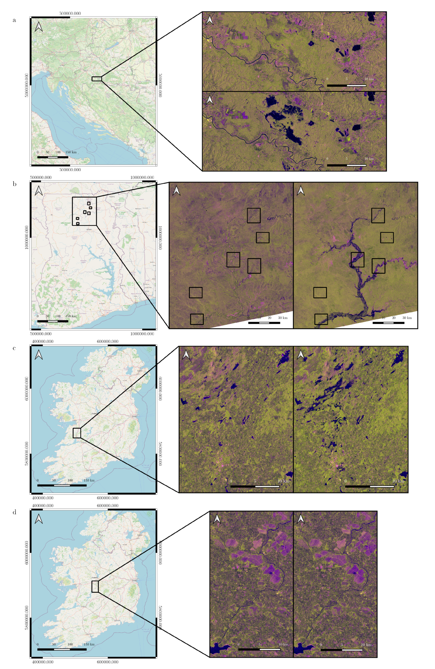
2.1. Study Cases
2.2. Data
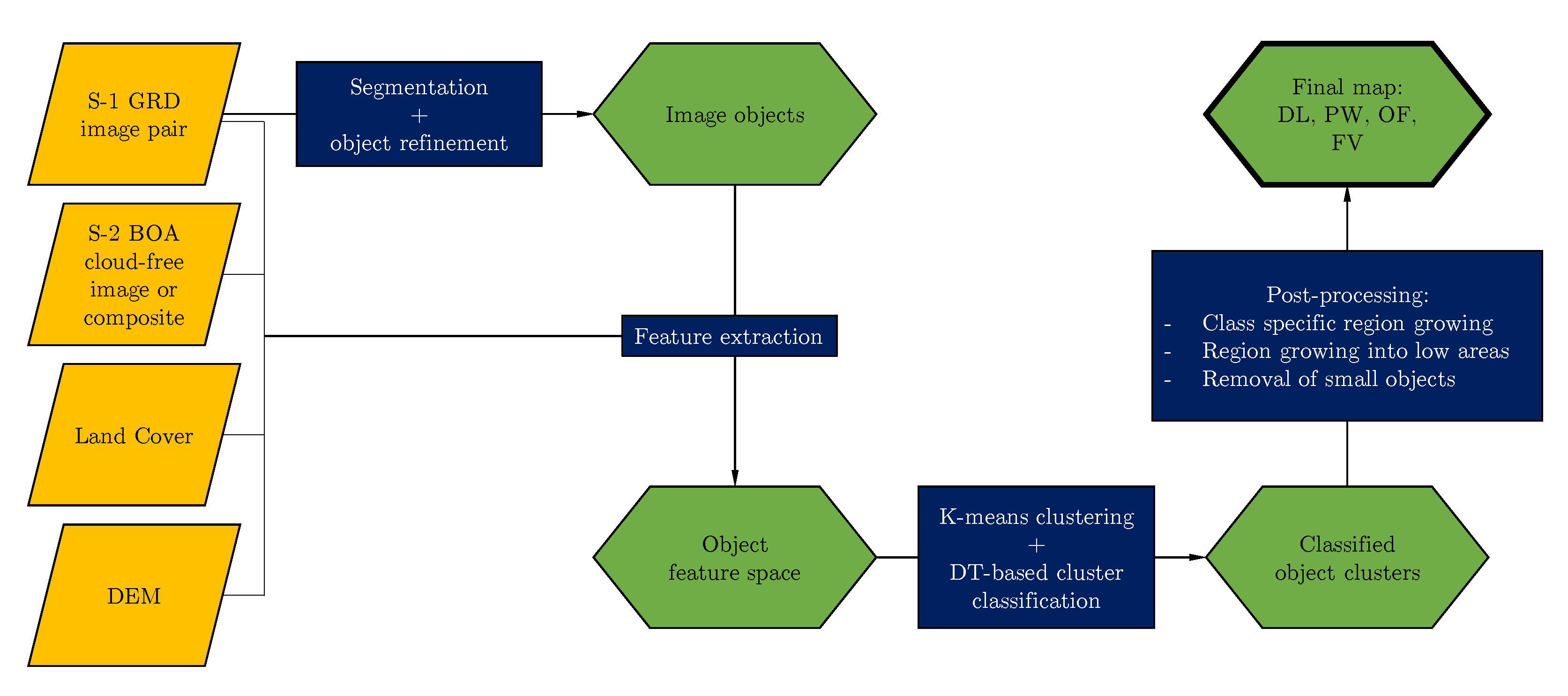
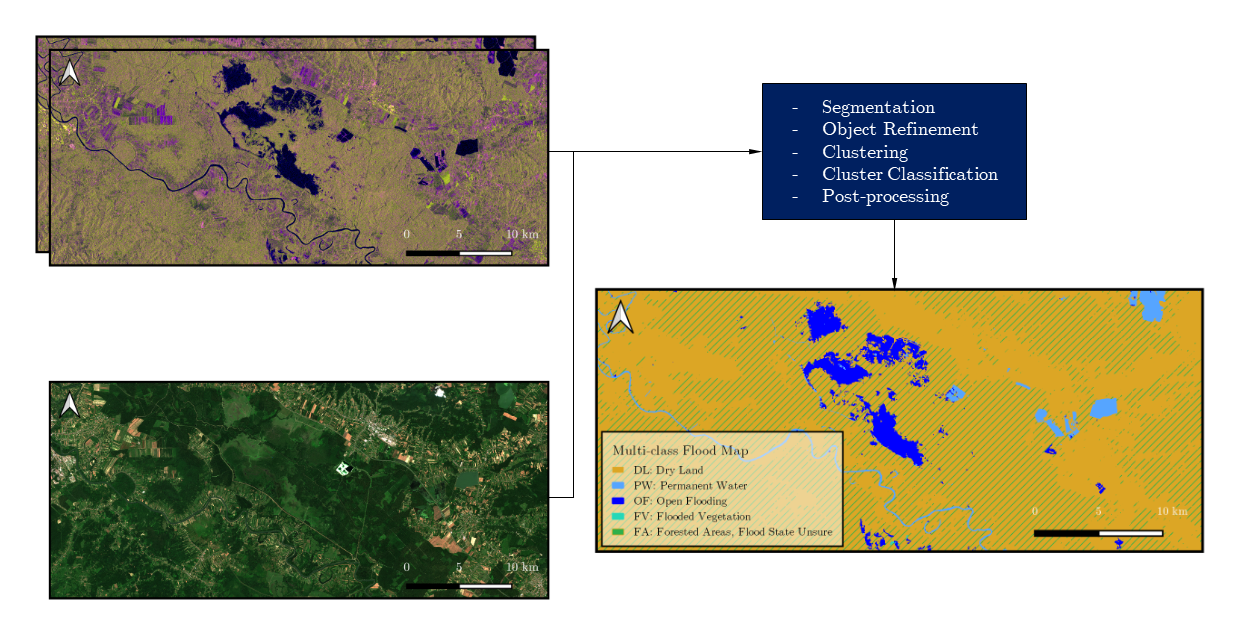
3. Methods
3.1. Image Segmentation Using the Quickshift Algorithm
3.2. Object-Based Clustering
3.3. Cluster Classification
3.4. Post-Processing Refinement
3.5. Accuracy Assessment
4. Results and Discussion
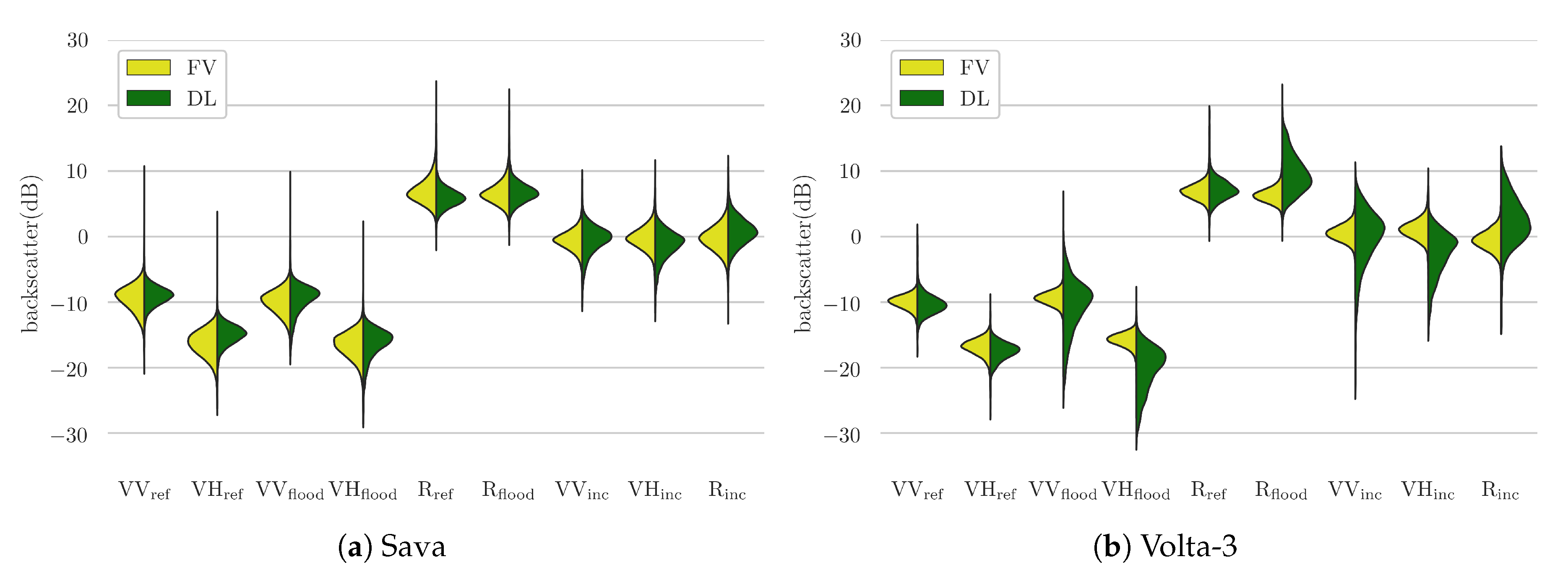
4.1. Separability of Flooded Vegetation
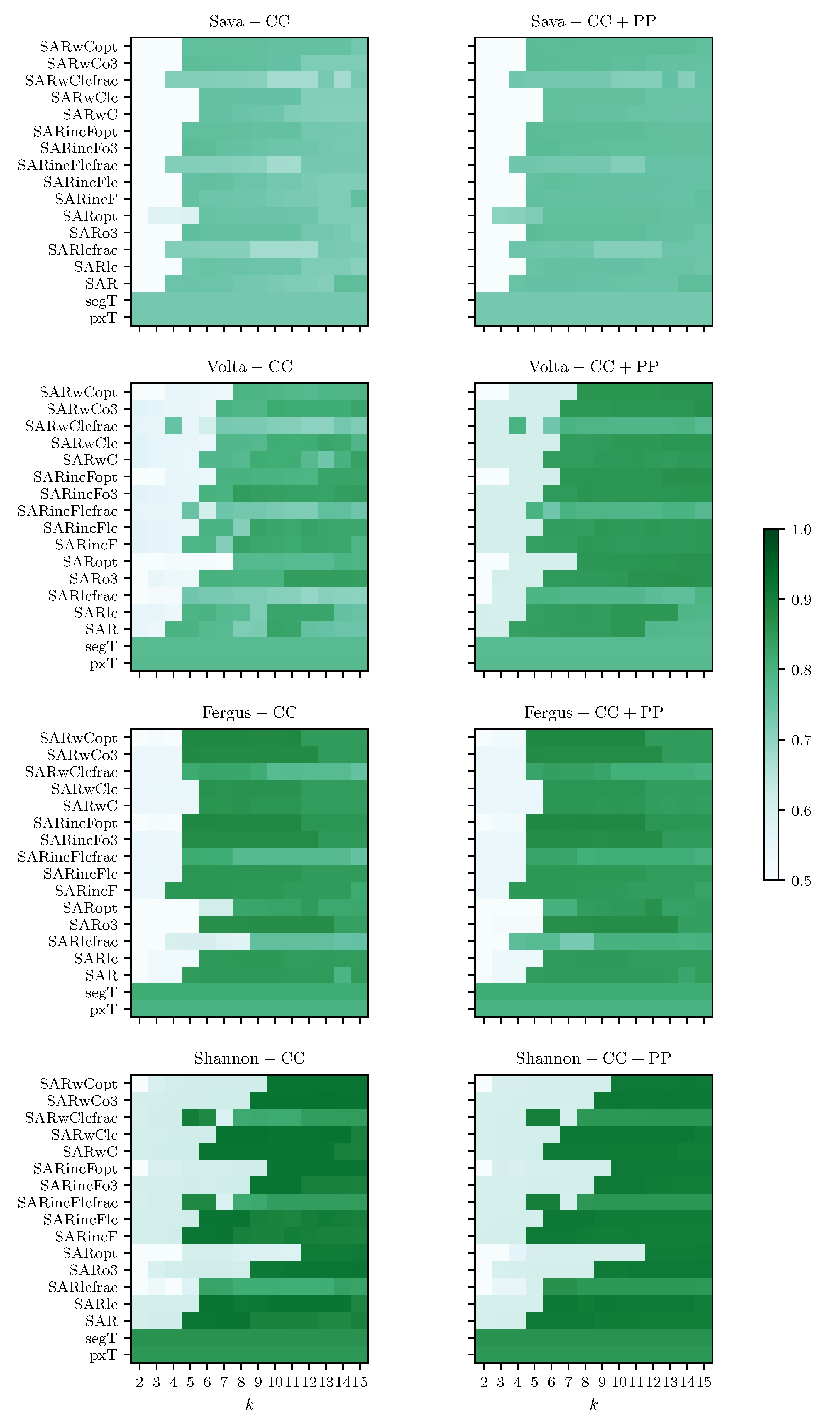
4.2. K-Means Cluster Classification
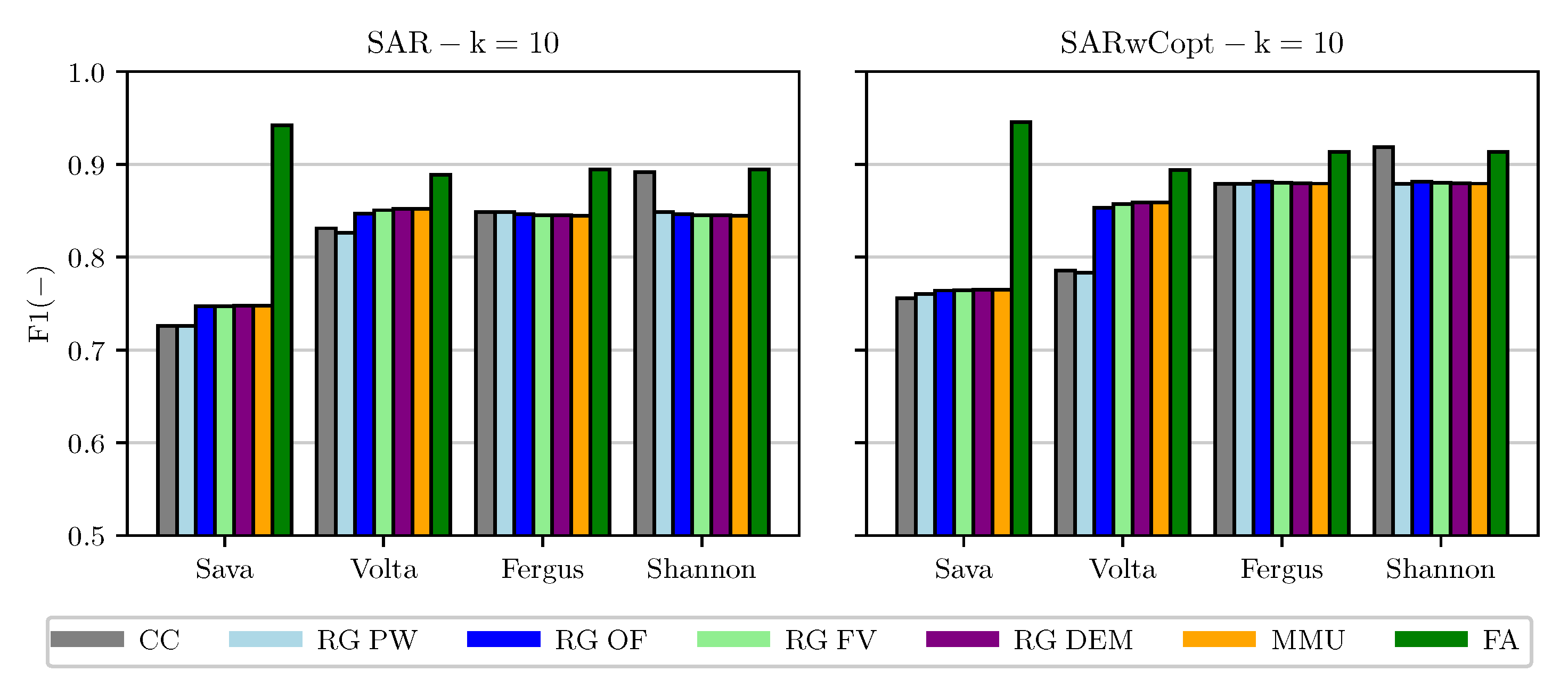
4.3. Post-Processing Refinement
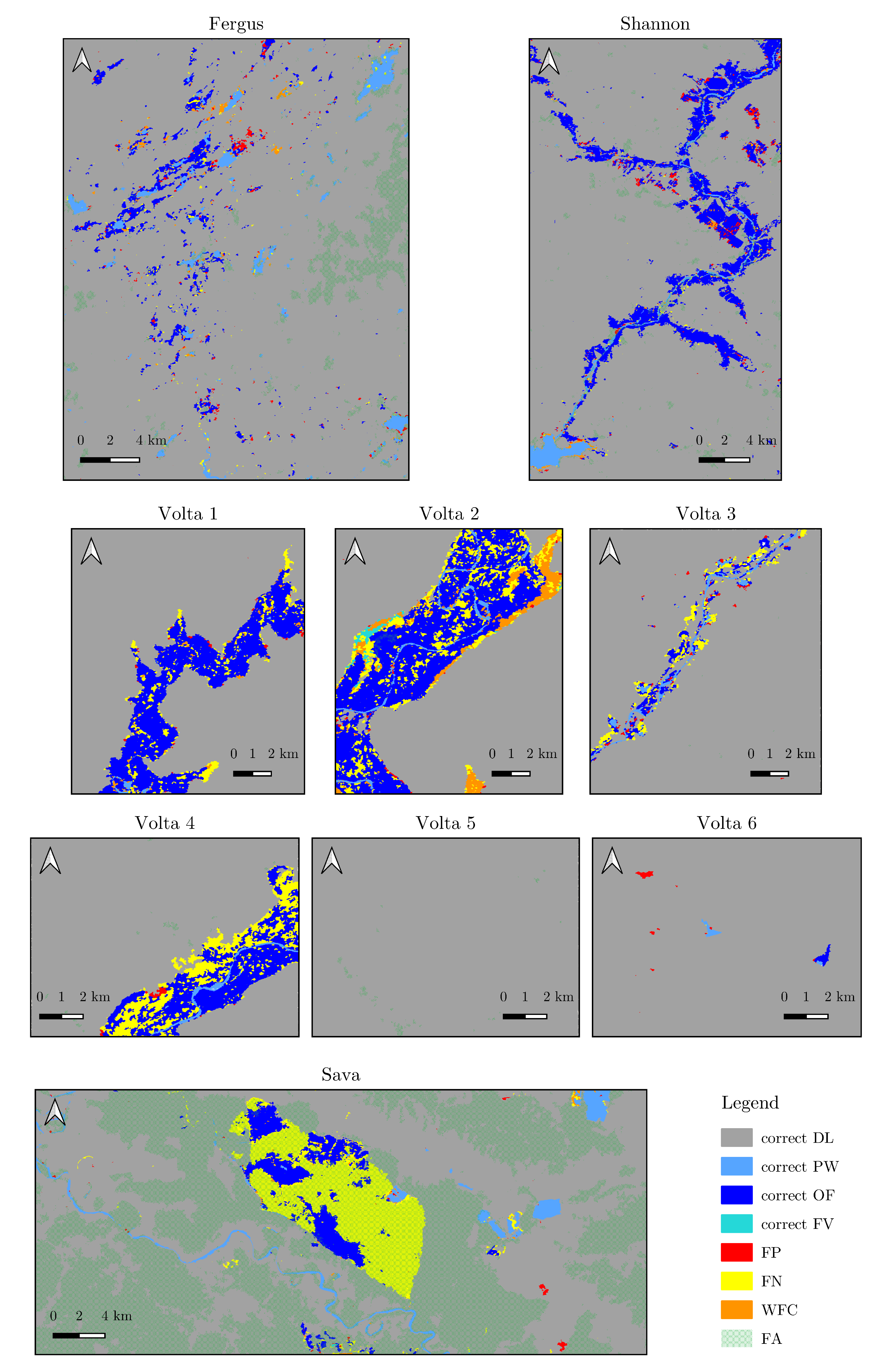
4.4. Final Flood Maps
4.5. Limitations and Future Improvements
5. Conclusions
Author Contributions
Funding
Acknowledgments
Conflicts of Interest
Abbreviations
| CGLS | Copernicus Global Land Service |
| DEM | Digital Elevation Model |
| DL | dry land |
| ESA | European Space Agency |
| FA | forested areas |
| FV | flooded vegetation |
| FS | feature space |
| OF | open flood |
| LC | land cover |
| MMU | minimal mapping unit |
| PW | permanent water |
| RG | region growing |
| ROI | region of interest |
| S-1 | Sentinel-1 |
| S-2 | Sentinel-2 |
| SAR | Synthetic Aperture Radar |
| SRTM | Shuttle Radar Topography Mission |
References
- Centre for Research on the Epidemiology of Disasters (CRED); United Nations Office for Disaster Risk Reduction (UNISDR). The Human Cost of Weather-Related Disasters 1995–2015. 2015. Available online: https://www.cred.be/sites/default/files/HCWRD_2015.pdf (accessed on 30 July 2020).
- Centre for Research on the Epidemiology of Disasters (CRED). Natural Disasters 2019. 2020. Available online: https://emdat.be/sites/default/files/adsr_2019.pdf (accessed on 30 July 2020).
- Milly, P.C.D.; Wetherald, R.T.; Dunne, K.; Delworth, T.L. Increasing risk of great floods in a changing climate. Nature 2002, 415, 514–517. [Google Scholar] [CrossRef] [PubMed]
- Voigt, S.; Giulio-Tonolo, F.; Lyons, J.; Kučera, J.; Jones, B.; Schneiderhan, T.; Platzeck, G.; Kaku, K.; Hazarika, M.K.; Czaran, L.; et al. Global trends in satellite-based emergency mapping. Science 2016, 353, 247–252. [Google Scholar] [CrossRef] [PubMed]
- Plank, S. Rapid Damage Assessment by Means of Multi-Temporal SAR—A Comprehensive Review and Outlook to Sentinel-1. Remote Sens. 2014, 6, 4870–4906. [Google Scholar] [CrossRef] [Green Version]
- Van Wesemael, A.; Verhoest, N.E.C.; Lievens, H. Assessing the Value of Remote Sensing and In Situ Data for Flood Inundation Forecasts. Ph.D. Thesis, Ghent University, Ghent, Belgium, 2019. [Google Scholar]
- Woodhouse, I.H. Introduction to Microwave Remote Sensing; CRC Press: Boca Raton, FL, USA, 2005. [Google Scholar] [CrossRef]
- Meyer, F. Spaceborne Synthetic Aperture Radar: Principles, Data Access, and Basic Processing Techniques. In The SAR Handbook: Comprehensive Methodologies for Forest Monitoring and Biomass Estimation; NASA: Washington, DC, USA, 2019; Chapter 1. [Google Scholar]
- Adeli, S.; Salehi, B.; Mahdianpari, M.; Quackenbush, L.J.; Brisco, B.; Tamiminia, H.; Shaw, S. Wetland Monitoring Using SAR Data: A Meta-Analysis and Comprehensive Review. Remote Sens. 2020, 12, 2190. [Google Scholar] [CrossRef]
- Grimaldi, S.; Li, Y.; Pauwels, V.R.N.; Walker, J.P. Remote Sensing-Derived Water Extent and Level to Constrain Hydraulic Flood Forecasting Models: Opportunities and Challenges. Surv. Geophys. 2016, 37, 977–1034. [Google Scholar] [CrossRef]
- Schumann, G.; Di Baldassarre, G.; Bates, P.D. The Utility of Spaceborne Radar to Render Flood Inundation Maps Based on Multialgorithm Ensembles. IEEE Trans. Geosci. Remote Sens. 2009, 47, 2801–2807. [Google Scholar] [CrossRef]
- Twele, A.; Cao, W.; Plank, S.; Martinis, S. Sentinel-1-based flood mapping: A fully automated processing chain. Int. J. Remote Sens. 2016, 37, 2990–3004. [Google Scholar] [CrossRef]
- Matgen, P.; Hostache, R.; Schumann, G.; Pfister, L.; Hoffmann, L.; Savenije, H. Towards an automated SAR-based flood monitoring system: Lessons learned from two case studies. Phys. Chem. Earth Parts A/B/C 2011, 36, 241–252. [Google Scholar] [CrossRef]
- Long, S.; Fatoyinbo, T.E.; Policelli, F. Flood extent mapping for Namibia using change detection and thresholding with SAR. Environ. Res. Lett. 2014, 9, 035002. [Google Scholar] [CrossRef]
- Li, Y.; Martinis, S.; Plank, S.; Ludwig, R. An automatic change detection approach for rapid flood mapping in Sentinel-1 SAR data. Int. J. Appl. Earth Obs. Geoinf. 2018, 73, 123–135. [Google Scholar] [CrossRef]
- Dasgupta, A.; Grimaldi, S.; Ramsankaran, R.; Pauwels, V.R.; Walker, J.P. Towards operational SAR-based flood mapping using neuro-fuzzy texture-based approaches. Remote Sens. Environ. 2018, 215, 313–329. [Google Scholar] [CrossRef]
- Amitrano, D.; Di Martino, G.; Iodice, A.; Riccio, D.; Ruello, G. Unsupervised Rapid Flood Mapping Using Sentinel-1 GRD SAR Images. IEEE Trans. Geosci. Remote Sens. 2018, 56, 3290–3299. [Google Scholar] [CrossRef]
- Schlaffer, S.; Chini, M.; Giustarini, L.; Matgen, P. Probabilistic mapping of flood-induced backscatter changes in SAR time series. Int. J. Appl. Earth Obs. Geoinf. 2017, 56, 77–87. [Google Scholar] [CrossRef]
- Tsyganskaya, V.; Martinis, S.; Marzahn, P.; Ludwig, R. Detection of temporary flooded vegetation using Sentinel-1 time series data. Remote Sens. 2018, 10, 1286. [Google Scholar] [CrossRef] [Green Version]
- Markert, K.N.; Chishtie, F.; Anderson, E.R.; Saah, D.; Griffin, R.E. On the merging of optical and SAR satellite imagery for surface water mapping applications. Results Phys. 2018, 9, 275–277. [Google Scholar] [CrossRef]
- DeVries, B.; Huang, C.; Armston, J.; Huang, W.; Jones, J.W.; Lang, M.W. Rapid and robust monitoring of flood events using Sentinel-1 and Landsat data on the Google Earth Engine. Remote Sens. Environ. 2020, 240, 111664. [Google Scholar] [CrossRef]
- Huang, W.; DeVries, B.; Huang, C.; Lang, M.; Jones, J.; Creed, I.; Carroll, M. Automated Extraction of Surface Water Extent from Sentinel-1 Data. Remote Sens. 2018, 10, 797. [Google Scholar] [CrossRef] [Green Version]
- Bonafilia, D.; Tellman, B.; Anderson, T.; Issenberg, E. Sen1Floods11: A Georeferenced Dataset to Train and Test Deep Learning Flood Algorithms for Sentinel-1. In Proceedings of the IEEE/CVF Conference on Computer Vision and Pattern Recognition (CVPR) Workshops, Seattle, WA, USA, 14–19 June 2020. [Google Scholar]
- Pierdicca, N.; Pulvirenti, L.; Chini, M. Flood Mapping in Vegetated and Urban Areas and Other Challenges: Models and Methods. In Flood Monitoring through Remote Sensing; Springer International Publishing: Cham, Switzerland, 2018; pp. 135–179. [Google Scholar] [CrossRef]
- Mason, D.C.; Dance, S.L.; Vetra-Carvalho, S.; Cloke, H.L. Robust algorithm for detecting floodwater in urban areas using synthetic aperture radar images. J. Appl. Remote Sens. 2018, 12, 1–20. [Google Scholar] [CrossRef] [Green Version]
- Chini, M.; Pelich, R.; Pulvirenti, L.; Pierdicca, N.; Hostache, R.; Matgen, P. Sentinel-1 InSAR Coherence to Detect Floodwater in Urban Areas: Houston and Hurricane Harvey as a Test Case. Remote Sens. 2019, 11, 107. [Google Scholar] [CrossRef] [Green Version]
- Li, Y.; Martinis, S.; Wieland, M.; Schlaffer, S.; Natsuaki, R. Urban Flood Mapping Using SAR Intensity and Interferometric Coherence via Bayesian Network Fusion. Remote Sens. 2019, 11, 2231. [Google Scholar] [CrossRef] [Green Version]
- Brisco, B.; Kapfer, M.; Hirose, T.; Tedford, B.; Liu, J. Evaluation of C-band polarization diversity and polarimetry for wetland mapping. Can. J. Remote Sens. 2011, 37, 82–92. [Google Scholar] [CrossRef]
- Tsyganskaya, V.; Martinis, S.; Marzahn, P.; Ludwig, R. SAR-based detection of flooded vegetation—A review of characteristics and approaches. Int. J. Remote Sens. 2018, 39, 2255–2293. [Google Scholar] [CrossRef]
- Martinez, J.M.; Le Toan, T. Mapping of flood dynamics and spatial distribution of vegetation in the Amazon floodplain using multitemporal SAR data. Remote Sens. Environ. 2007, 108, 209–223. [Google Scholar] [CrossRef]
- Pistolesi, L.I.; Ni-Meister, W.; McDonald, K.C. Mapping wetlands in the Hudson Highlands ecoregion with ALOS PALSAR: An effort to identify potential swamp forest habitat for golden-winged warblers. Wetl. Ecol. Manag. 2015, 23, 95–112. [Google Scholar] [CrossRef]
- San Martín, L.S.; Morandeira, N.S.; Grimson, R.; Rajngewerc, M.; González, E.B.; Kandus, P. The contribution of ALOS/PALSAR-1 multi-temporal data to map permanently and temporarily flooded coastal wetlands. Int. J. Remote Sens. 2020, 41, 1582–1602. [Google Scholar] [CrossRef]
- Evans, T.L.; Costa, M.; Telmer, K.; Silva, T.S.F. Using ALOS/PALSAR and RADARSAT-2 to Map Land Cover and Seasonal Inundation in the Brazilian Pantanal. IEEE J. Sel. Top. Appl. Earth Obs. Remote Sens. 2010, 3, 560–575. [Google Scholar] [CrossRef]
- Townsend, P.A. Mapping seasonal flooding in forested wetlands using multi-temporal Radarsat SAR. Photogramm. Eng. Remote Sens. 2001, 67, 857–864. [Google Scholar]
- Voormansik, K.; Praks, J.; Antropov, O.; Jagomägi, J.; Zalite, K. Flood Mapping with TerraSAR-X in Forested Regions in Estonia. IEEE J. Sel. Top. Appl. Earth Obs. Remote Sens. 2014, 7, 562–577. [Google Scholar] [CrossRef]
- Hess, L.L.; Melack, J.M. Remote sensing of vegetation and flooding on Magela Creek Floodplain (Northern Territory, Australia) with the SIR-C synthetic aperture radar. In Aquatic Biodiversity: A Celebratory Volume in Honour of Henri J. Dumont; Springer: Dordrecht, The Netherlands, 2003; pp. 65–82. [Google Scholar] [CrossRef]
- Lang, M.W.; Townsend, P.A.; Kasischke, E.S. Influence of incidence angle on detecting flooded forests using C-HH synthetic aperture radar data. Remote Sens. Environ. 2008, 112, 3898–3907. [Google Scholar] [CrossRef]
- Richards, J.A.; Woodgate, P.W.; Skidmore, A.K. An explanation of enhanced radar backscattering from flooded forests. Int. J. Remote Sens. 1987, 8, 1093–1100. [Google Scholar] [CrossRef]
- Töyrä, J.; Pietroniro, A.; Martz, L.W. Multisensor Hydrologic Assessment of a Freshwater Wetland. Remote Sens. Environ. 2001, 75, 162–173. [Google Scholar] [CrossRef]
- Refice, A.; Zingaro, M.; D’Addabbo, A.; Chini, M. Integrating C- and L-Band SAR Imagery for Detailed Flood Monitoring of Remote Vegetated Areas. Water 2020, 10, 2745. [Google Scholar] [CrossRef]
- Martinis, S.; Rieke, C. Backscatter Analysis Using Multi-Temporal and Multi-Frequency SAR Data in the Context of Flood Mapping at River Saale, Germany. Remote Sens. 2015, 7, 7732–7752. [Google Scholar] [CrossRef] [Green Version]
- Brisco, B.; Shelat, Y.; Murnaghan, K.; Montgomery, J.; Fuss, C.; Olthof, I.; Hopkinson, C.; Deschamps, A.; Poncos, V. Evaluation of C-Band SAR for Identification of Flooded Vegetation in Emergency Response Products. Can. J. Remote Sens. 2019, 45, 73–87. [Google Scholar] [CrossRef]
- Chaabani, C.; Chini, M.; Abdelfattah, R.; Hostache, R.; Chokmani, K. Flood Mapping in a Complex Environment Using Bistatic TanDEM-X/TerraSAR-X InSAR Coherence. Remote Sens. 2018, 10, 1873. [Google Scholar] [CrossRef] [Green Version]
- Pulvirenti, L.; Chini, M.; Pierdicca, N.; Boni, G. Use of SAR Data for Detecting Floodwater in Urban and Agricultural Areas: The Role of the Interferometric Coherence. IEEE Trans. Geosci. Remote Sens. 2016, 54, 1532–1544. [Google Scholar] [CrossRef]
- Zhang, M.; Li, Z.; Tian, B.; Zhou, J.; Zeng, J. A method for monitoring hydrological conditions beneath herbaceous wetlands using multi-temporal ALOS PALSAR coherence data. Remote Sens. Lett. 2015, 6, 618–627. [Google Scholar] [CrossRef]
- Brisco, B.; Schmitt, A.; Murnaghan, K.; Kaya, S.; Roth, A. SAR polarimetric change detection for flooded vegetation. Int. J. Digit. Earth 2013, 6, 103–114. [Google Scholar] [CrossRef]
- Plank, S.; Jüssi, M.; Martinis, S.; Twele, A. Mapping of flooded vegetation by means of polarimetric Sentinel-1 and ALOS-2/PALSAR-2 imagery. Int. J. Remote Sens. 2017, 38, 3831–3850. [Google Scholar] [CrossRef]
- Tsyganskaya, V.; Martinis, S.; Marzahn, P. Flood Monitoring in Vegetated Areas Using Multitemporal Sentinel-1 Data: Impact of Time Series Features. Water 2019, 11, 1938. [Google Scholar] [CrossRef] [Green Version]
- Olthof, I.; Tolszczuk-Leclerc, S. Comparing Landsat and RADARSAT for Current and Historical Dynamic Flood Mapping. Remote Sens. 2018, 10, 780. [Google Scholar] [CrossRef] [Green Version]
- Pierdicca, N.; Pulvirenti, L.; Boni, G.; Squicciarino, G.; Chini, M. Mapping Flooded Vegetation Using COSMO-SkyMed: Comparison With Polarimetric and Optical Data Over Rice Fields. IEEE J. Sel. Top. Appl. Earth Obs. Remote Sens. 2017, 10, 2650–2662. [Google Scholar] [CrossRef]
- Grimaldi, S.; Xu, J.; Li, Y.; Pauwels, V.R.; Walker, J.P. Flood mapping under vegetation using single SAR acquisitions. Remote Sens. Environ. 2020, 237, 111582. [Google Scholar] [CrossRef]
- International Federation of Red Cross (IFRC); Red Crescent Societies. Ghana: Floods in Upper East Region—Emergency Plan of Action Final Report; IFRC: Geneva, Switzerland, 2019. [Google Scholar]
- Campanyà i Llovet, J.; McCormack, T.; Naughton, O. Remote Sensing for Monitoring and Mapping Karst Groundwater Flooding in the Republic of Ireland. In Proceedings of the EGU General Assembly 2020, Vienna, Austria, 4–8 May 2020; p. 18921. [Google Scholar] [CrossRef]
- Copernicus Emergency Management Service (©2015 European Union), EMSR149.
- Buchhorn, M.; Lesiv, M.; Tsendbazar, N.E.; Herold, M.; Bertels, L.; Smets, B. Copernicus Global Land Cover Layers—Collection 2. Remote Sens. 2020, 12, 1044. [Google Scholar] [CrossRef] [Green Version]
- Hostache, R.; Matgen, P.; Wagner, W. Change detection approaches for flood extent mapping: How to select the most adequate reference image from online archives? Int. J. Appl. Earth Obs. Geoinf. 2012, 19, 205–213. [Google Scholar] [CrossRef]
- Simonetti, D.; Simonetti, E.; Szantoi, Z.; Lupi, A.; Eva, H.D. First Results From the Phenology-Based Synthesis Classifier Using Landsat 8 Imagery. IEEE Geosci. Remote Sens. Lett. 2015, 12, 1496–1500. [Google Scholar] [CrossRef]
- Lehner, B.; Verdin, K.; Jarvis, A. New Global Hydrography Derived From Spaceborne Elevation Data. Eos Trans. Am. Geophys. Union 2008, 89, 93–94. [Google Scholar] [CrossRef]
- Vedaldi, A.; Soatto, S. Quick shift and kernel methods for mode seeking. In European Conference on Computer Vision; Springer: Berlin/Heidelberg, Germany, 2008; pp. 705–718. [Google Scholar] [CrossRef] [Green Version]
- Hartigan, J.A.; Wong, M.A. Algorithm AS 136: A k-means clustering algorithm. J. R. Stat. Soc. Ser. C Appl. Stat. 1979, 28, 100–108. [Google Scholar] [CrossRef]
- Landuyt, L.; Van Wesemael, A.; Schumann, G.J.P.; Hostache, R.; Verhoest, N.E.C.; Van Coillie, F.M.B. Flood Mapping Based on Synthetic Aperture Radar: An Assessment of Established Approaches. IEEE Trans. Geosci. Remote Sens. 2019, 57, 722–739. [Google Scholar] [CrossRef]
- Debusscher, B.; Van Coillie, F. Object-Based Flood Analysis Using a Graph-Based Representation. Remote Sens. 2019, 11, 1883. [Google Scholar] [CrossRef] [Green Version]
- Stephens, E.; Schumann, G.; Bates, P. Problems with binary pattern measures for flood model evaluation. Hydrol. Process. 2014, 28, 4928–4937. [Google Scholar] [CrossRef]
- Weydahl, D.J.; Sagstuen, J.; Dick, O.B.; Rønning, H. SRTM DEM accuracy assessment over vegetated areas in Norway. Int. J. Remote Sens. 2007, 28, 3513–3527. [Google Scholar] [CrossRef]
- Olthof, I.; Rainville, T. Evaluating Simulated RADARSAT Constellation Mission (RCM) Compact Polarimetry for Open-Water and Flooded-Vegetation Wetland Mapping. Remote Sens. 2020, 12, 1476. [Google Scholar] [CrossRef]
- Jet Propulsion Laboratory (JPL). NISAR: Mission Concept. Available online: https://nisar.jpl.nasa.gov/mission/mission-concept/ (accessed on 1 September 2020).
- Pierdicca, N.; Davidson, M.; Chini, M.; Dierking, W.; Djavidnia, S.; Haarpaintner, J.; Hajduch, G.; Laurin, G.V.; Lavalle, M.; López-Martínez, C.; et al. The Copernicus L-band SAR mission ROSE-L (Radar Observing System for Europe) (Conference Presentation). In Proceedings of the SPIE Remote Sensing—Active and Passive Microwave Remote Sensing for Environmental Monitoring, Strasbourg, France, 9–12 September 2019. [Google Scholar] [CrossRef]
- Chini, M.; Hostache, R.; Giustarini, L.; Matgen, P. A Hierarchical Split-Based Approach for Parametric Thresholding of SAR Images: Flood Inundation as a Test Case. IEEE Trans. Geosci. Remote Sens. 2017, 55, 6975–6988. [Google Scholar] [CrossRef]
- Esch, T.; Bachofer, F.; Heldens, W.; Hirner, A.; Marconcini, M.; Palacios-Lopez, D.; Roth, A.; Üreyen, S.; Zeidler, J.; Dech, S.; et al. Where We Live—A Summary of the Achievements and Planned Evolution of the Global Urban Footprint. Remote Sens. 2018, 10, 895. [Google Scholar] [CrossRef] [Green Version]


| Study Area | S-1 Ref. Image | S-1 Flood Image | S-2 CFC Date Range |
|---|---|---|---|
| Sava | 9 May 2019 | 8 June 2019 | 17 July 2019 |
| Volta | 1 August 2018 | 18 September 2018 | 1 May–1 August 2018 |
| Fergus | 29 October 2015 | 16 December 2015 | 1 September–1 December 2016 |
| Shannon | 29 October 2015 | 9 January 2016 | 1 September–1 December 2016 |
| Feature Subspace | Bands | Band Description |
|---|---|---|
| SAR | , , , | VV and VH band of the reference and flood S-1 image |
| wC | , , , , | ratio (linear scale) of VV and VH band of reference and flood S-1 image; increase of VV, VH and R band between reference and flood S-1 image |
| incF | , , | increase of VV, VH and R band between reference and flood S-1 image |
| lc | LC | CGLS land cover class |
| lcfrac | , , , , , , , | CGLS land cover fractions for bare, grass, crops, shrubs, trees, permanent water, seasonal water and urban classes (cfr. Section 2.2) |
| o3 | , , | B4, B8 and B12 of S-2 image/composite |
| opt | , , , , , , , , , | B2, B3, B4, B5, B6, B7, B8, B9, B10, B11 and B12 of S-2 image/composite |
| Class | Seed Class | Source Class | Growing Condition |
|---|---|---|---|
| PW | PW | OF/DL | |
| OF | PW/OF/FV | DL | |
| FV | OF/FV | DL | |
| LL | PW/OF/FV | DL |
| Measure | Sava | Volta | Fergus | Shannon |
|---|---|---|---|---|
| F1 three-class | 0.7648 | 0.8588 | 0.8793 | 0.9098 |
| F1 single | 0.7467 | 0.9287 | 0.9461 | 0.9625 |
| F1 change | 0.7031 | 0.9117 | 0.8904 | 0.9449 |
Publisher’s Note: MDPI stays neutral with regard to jurisdictional claims in published maps and institutional affiliations. |
© 2020 by the authors. Licensee MDPI, Basel, Switzerland. This article is an open access article distributed under the terms and conditions of the Creative Commons Attribution (CC BY) license (http://creativecommons.org/licenses/by/4.0/).
Share and Cite
Landuyt, L.; Verhoest, N.E.C.; Van Coillie, F.M.B. Flood Mapping in Vegetated Areas Using an Unsupervised Clustering Approach on Sentinel-1 and -2 Imagery. Remote Sens. 2020, 12, 3611. https://doi.org/10.3390/rs12213611
Landuyt L, Verhoest NEC, Van Coillie FMB. Flood Mapping in Vegetated Areas Using an Unsupervised Clustering Approach on Sentinel-1 and -2 Imagery. Remote Sensing. 2020; 12(21):3611. https://doi.org/10.3390/rs12213611
Chicago/Turabian StyleLanduyt, Lisa, Niko E. C. Verhoest, and Frieke M. B. Van Coillie. 2020. "Flood Mapping in Vegetated Areas Using an Unsupervised Clustering Approach on Sentinel-1 and -2 Imagery" Remote Sensing 12, no. 21: 3611. https://doi.org/10.3390/rs12213611
APA StyleLanduyt, L., Verhoest, N. E. C., & Van Coillie, F. M. B. (2020). Flood Mapping in Vegetated Areas Using an Unsupervised Clustering Approach on Sentinel-1 and -2 Imagery. Remote Sensing, 12(21), 3611. https://doi.org/10.3390/rs12213611