Article

An OSM Data-Driven Method for Road-Positive Sample Creation

1
School of Geomatics, Liaoning Technical University, Fuxin 123000, China
2
Institute of Spatiotemporal Transportation Data, Liaoning Technical University, Fuxin 123000, China
3
Beijing Key Laboratory of Urban Spatial Information Engineering, Beijing 100038, China
4
China Land Surveying and Planning Institute, Beijing 100035, China
5
Key Laboratory of Surveying and Mapping Science and Geospatial Information Technology of Ministry of Natural Resources, Beijing 100036, China
6
The Chinese Academy of Surveying and Mapping, Beijing 100036, China
*
Author to whom correspondence should be addressed.
Remote Sens. 2020, 12(21), 3612; https://doi.org/10.3390/rs12213612
Submission received: 18 September 2020 / Revised: 30 October 2020 / Accepted: 2 November 2020 / Published: 3 November 2020

Abstract

:
Determining samples is considered to be a precondition in deep network training and learning, but at present, samples are usually created manually, which limits the application of deep networks. Therefore, this article proposes an OpenStreetMap (OSM) data-driven method for creating road-positive samples. First, based on the OSM data, a line segment orientation histogram (LSOH) model is constructed to determine the local road direction. Secondly, a road homogeneity constraint rule and road texture feature statistical model are constructed to extract the local road line, and on the basis of the local road lines with the same direction, a polar constraint rule is proposed to determine the local road line set. Then, an iterative interpolation algorithm is used to connect the local road lines on both sides of the gaps between the road lines. Finally, a local texture self-similarity (LTSS) model is implemented to determine the road width, and the centerpoint autocorrection model and random sample consensus (RANSAC) algorithm are used to extract the road centerline; the road width and road centerline are used to complete the creation of the road-positive samples. Experiments are conducted on different scenes and different types of images to demonstrate the proposed method and compare it with other approaches. The results demonstrate that the proposed method for creating road-positive samples has great advantages in terms of accuracy and integrity.

Graphical Abstract

1. Introduction

Extracting roads from high-resolution remote sensing images is an effective way to update road information, which can provide not only reference data for map updates [1] and traffic flow assignment [2] but also decision-making bases for vehicle navigation [3] and smart city planning [4]. Therefore, many scholars have performed research in this field. According to the time sequence of road extraction research, this article divides the road extraction methods into traditional methods and deep convolution neural network methods. Traditional methods construct the theoretical mathematical model and compute the solution. For example, considering a road’s geometric features, the road extraction methods include parallel edge [5,6], line segment [7], and path morphology [8]. Furthermore, Kass et al. [9] proposed a snake model, which fully uses the road geometric features and extracts roads by solving the extreme value of the energy function in a certain region. Considering the spectral texture homogeneity of a road, the classical method is an object-oriented method [10]. In this method, the road is regarded as a region with a certain geometric regularity and texture homogeneity. The road region is divided by segmentation, and the road is extracted by classification and post-processing methods.
Due to the complex environmental changes inside and outside a road, the automation and accuracy of the traditional methods are still deficient. With the advent of the era of artificial intelligence and deep learning, many scholars have turned to the study of deep networks for road extraction. A deep network mines image features based on a large number of samples and uses a discriminant function to predict the probability value of a road image at the pixel level. Since 2012, some scholars have introduced deep networks into the field of road extraction [11,12,13,14,15]. For example, Teerapong et al. [16] proposed an enhanced deep convolution neural network framework. The activation function of the exponential linear unit is embedded into the neural network to extract roads, and then a method based on landscape measurement and a conditional random field is used to improve the accuracy of the road extraction. Through the training of the image sample sets, the deep network can effectively solve the occlusion problem in road extraction [13,17,18,19]. At present, the sample creating is usually performed manually, which often leads to a shortage of sample sets, and reduces the performance of the deep learning [17,18,19,20].
At present, there are three types of sample creating methods, namely, strong supervised learning, weak supervised learning, and semi supervised learning. Among them, strong supervised learning simplifies the problems in the real scene, which means that it does not hold true in many real scenes. What we get in real scenes is relatively weak supervision information, so weak supervised learning and semi supervised learning have been widely considered by researchers [21,22,23]. Generally, weak supervision can be classified into incomplete supervision, imprecise supervision, and inaccurate supervision. Semi supervised learning uses a small number of labeled samples and a large number of unlabeled samples to train the classification model. Semi supervised learning is mainly divided into the four categories of a generative-based method [24,25], low density segmentation-based method [26,27], divergence-based method [28,29], and graph-based method [21,22,23]. The above methods are based on the existing samples, but the problem of creating samples without prior samples has not been discussed in depth.
In recent years, with the help of Web2.0, more and more volunteers are creating voluntary geographic information (VGI). VGI includes OSM data, GPS data, navigation data, etc. Some researchers have attempted to extract roads from existing geographic data [30,31,32]. For example, Cao and Sun [31] determined the candidate road seed points through an analysis of GPS points, ascertained the segmentation peak perpendicular to the road by filtering and difference, established the road centerpoint through the gray mean value and segmentation size, and connected the road centerpoints to form the road centerline. The above methods can extract roads from geographic data, but the extracted roads are misclassified or fractured, which leads to the low accuracy of extraction and sometimes requires manual participation. OSM is the most influential and far-reaching project in VGI, where volunteers share map data all over the world by using crowdsourcing. The volunteers who participate in the project do not necessarily have the professional qualifications or background in the field of geographic data collection or measurement. Consequently, these data may not necessarily meet professional standards in terms of accuracy [33]. However, considering that OSM data can provide some initial road information, some scholars turn to OSM data to extract roads [32,33,34,35]. For example, Li et al. [32] proposed a method for extracting highway networks from OSM data. However, due to the complexity of road structures, this method easily identifies non-roads as multi-lane roads. Compared with other geographic data, OSM data cover a wide range and are easy to obtain. Therefore, inspired by the road extraction that uses OSM data, to solve the problems of the current road sample creation described above, we propose an OSM data-driven method for road-positive sample creation. The rest of the article is arranged as follows: Section 2 introduces the materials and methods; Section 3 describes the experimental analysis and evaluation; a discussion is presented in Section 4; and a summary and future work are described in Section 5.

2. Materials and Method

2.1. Experimental Data

The proposed method is based on panchromatic high-resolution remote sensing images with a resolution of less than 1 m and their corresponding OSM data. The algorithms were implemented in C ++ by using the Visual Studio 2013 platform. The input remote sensing images are orthophoto images generated through pixel-by-pixel correction, mosaics, and clipping. Orthophoto has the characteristics of a high geometric accuracy, rich image information, and intuitive reality [36]. The orthophoto images in Experiments 1 and 2 were provided by Beijing Longyufangyuan Information Technology Co., Ltd., and the orthophoto images in Experiment 3 were provided by Beijing Guocexinghui Information Technology Co., Ltd. Their corresponding OSM data were downloaded at the same time from https://www.openstreetmap.org/.
To verify the effectiveness and universality of the method, considering that the OSM data in densely populated areas are generally more accurate than that in sparsely populated areas [37], and the road types between urban and rural areas are different, the following three ortho-corrected images covering urban, rural, and suburban areas were selected for the experiments.
The image shown for Experiment 1 (urban area) is a remote sensing image of the GeoEye-1 optical satellite that covers the urban area of Hobart, Australia, and was taken in February 2009 (leaf-on). The image size is 5000 × 5000 pixels with a spatial resolution of 0.41 m and the WGS-84 coordinate system. The roads in the image may be hidden by a small amount of vehicle noise, shadow shading, and the local road width has continuous change phenomenon. To verify the effectiveness of the proposed method, Experiment 1 images were selected as data for the comparative experiment. We compared the method with the deep learning model [13,38]. It is mainly considered that the current methods are usually based on prior samples for sample enhancement. However, our method is based on no prior samples to create samples automatically, which leads to less comparison methods. The proposed method was implemented using a PC with an NVIDIA GTX 1060TI and 8 GB of onboard memory. This image was cut into 1521 images according to the size of 128 × 128 pixels. After image reverse and rotation data enhancement, 3240 images were generated. These images were divided into 10 samples, of which 90% of the images (2916 images) were used as the training set, and the remaining 324 images constituted the verification set. The test set contained an image with a resolution of 5000 × 5000 pixels.
The image shown for Experiment 2 (rural area) is a remote sensing image of the high-view optical satellite that covers the rural area of Huludao, China, and was taken in August 2017 (leaf-on). The image size is 2000 × 2000 pixels with a spatial resolution of 0.5 m and a WGS-84 coordinate system. Compared with urban roads, the characteristics of rural roads in the image show the larger curvature of the local roads.
The image shown for Experiment 3 (suburban area) is a remote sensing image of the GF2 optical satellite that covers the suburban area of Huludao, China, and was taken in July 2015 (leaf-on). The image size is 3000 × 3000 pixels with a spatial resolution of 0.81 m and a WGS-84 coordinate system. The image contains two different types of roads, specifically, urban roads and provincial roads.

2.2. Methodology

Inconsistencies in orientation and position appear when the OSM is superimposed on the orthophotos. These inconsistencies cannot be ignored as they will reduce the reliability of the road-positive samples. Hence, to obtain more reliable road-positive samples, with regard to the proposed method of the article, we (a) propose in Section 2.2.1 an LSOH model to determine the local road direction; (b) in Section 2.2.2 propose the road homogeneity constraint rules, road texture feature statistical model, and polar constraint rule to extract the local road line set; (c) in Section 2.2.3 the iterative interpolation algorithm is used to connect the local road lines on both sides of the gaps between the road lines; and (d) in Section 2.2.4 an LTSS model, a centerpoint autocorrection model, and the RANSAC algorithm are used in turn to extract the road width and road centerline to complete the creation of the road-positive samples. Figure 1 shows a flowchart of the proposed method.

2.2.1. Local Road Direction Determination

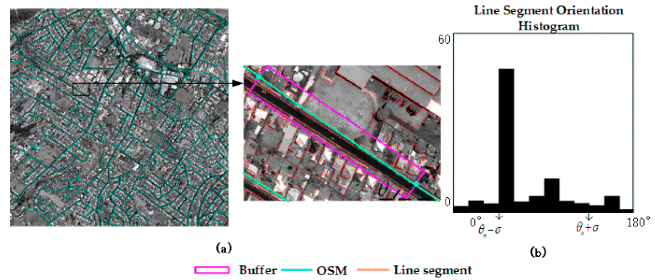
Since the direction indicated by the OSM data is not necessarily consistent with the road directions in the image, it is necessary to adjust them. The line segment between a pair of adjacent nodes of OSM data is defined as the local OSM vector, and the local road direction is consistent with the corrected direction of local OSM vector in the proposed method. Generally, there is a certain relationship between the road direction and the edge information in the road neighborhood. For example, the edge information of the indication line in the road, the motor vehicle, the separation zone, and buildings are consistent with the road direction. Therefore, from the perspective of road geometric characteristics, an LSOH model is proposed to adjust the direction of the OSM data to the road direction in the Figure 2.
(1) Buffer settings
In OSM data, roads are usually organized and expressed in the form of connected nodes. In the proposed method, the local OSM vector is used as the buffer axis. The statistical analysis of a large number of OSM data and road images shows that, in our case, the error between them is usually less than 3 m. Therefore, Equation (1) is used to determine the buffer width in the proposed method:
w = 2 W 0 / r
where w is the buffer width, W0 is 3 m, and r is the image spatial resolution.
(2) LSOH model
Figure 2a shows the overlay of OSM data and the line segment extraction results with the image and a locally enlarged image. The red line segment is the result extracted from the remote sensing image by using the line extraction method for chain code tracking with phase verification [39]. In the buffer, the road, buildings, and other features provide a large number of edges. In the road direction, the road edges provide a long line segment, while in the non-road direction, the edges of the buildings and other features are short line segments. Accordingly, the LSOH model is constructed by counting the length of the line segment from different orientations and adding it to the line segment orientation histogram. The error between the OSM data direction and the road direction in the image is small; therefore, the angle constraint threshold σ is set. Based on the OSM data direction θn, the line segments within the range of [θnσ, θn + σ] are analyzed. The angle constraint threshold σ setting is shown in detail in the parameter settings of Section 3.2. Figure 2b shows the LSOH model. It is constructed with the angle of the line segment as the X-axis, the magnitude unit is γ, the range is 0–180°, and the accumulated length of the line segment from different orientations in the buffer represents the Y-axis. The magnitude unit γ is shown in detail in the parameter settings of Section 3.2. To ensure the accuracy of the local road direction and avoid the interference of other features, the statistical peak of the orientation provided by the model is constrained in the proposed method as follows. When Equation (2) is satisfied, the peak of the angle is the local road direction.
H F λ H S
where HF is the maximum peak in the LSOH model, HS is the secondary peak, and λ is the scale factor. The scale factor λ is shown in detail in the parameter settings of Section 3.2.

2.2.2. Local Road Line Set Extraction

As an artificial ground object, roads generally have texture homogeneity and linear geometric characteristics [40]. However, in an image, roads may be hidden by vehicles (traffic noise), shadow from surrounding buildings, or other phenomena. Therefore, based on the local road direction determination, the following steps are carried out to extract the local road line set: the road homogeneity constraint rule; the road texture feature statistical model; and local road line set extraction. A road segment in the image corresponding to the local OSM vector is defined as the local road line, and several adjacent local road lines with the same direction constitute the local road line set.
(1) Road homogeneity constraint rule
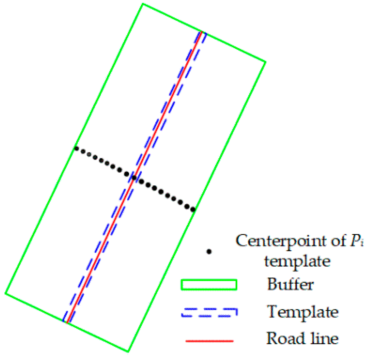
According to the idea that the road homogeneity is higher than that of adjacent features, the candidate local road line buffer is first constructed in the proposed method, which takes the corrected local OSM vector as the symmetry axis and w as the width, where w is calculated by Equation (1). In the buffer, based on the centerpoint of the corrected local OSM vector and by taking the corrected local OSM vector as the symmetry axis, a template with a width of 1 is constructed, as shown in Figure 3. Then, along the direction perpendicular to the local road direction, the template is then selected in Step 1. Consequently, the black point in Figure 3 is the centerpoint of the template, which forms the candidate local road line template set V, where V = {V1, V2... Vi... Vn}. The texture variance TFVi and image mean value Gi of the Vi template are calculated, TFVi are ordered from smallest to largest, the minimum value TFVmin and its corresponding Vi are determined, and TFVmin and the image mean value Gi of Vi are tracked. Meanwhile, the secondary minimum value TFVn_min and Gn_i are tracked, where Gi and Gn_i should satisfy Equation (3).
G n _ i G i η
where Gn_i is the TFVn_min corresponding to the image mean value, and η represents the constraint threshold of the image value. The constraint threshold of image values η is shown in detail in the parameter settings of Section 3.2.
(2) Road texture feature statistical model
In most cases, the pavement material is the same or similar and has similar texture feature information. Sometimes, in an image, local roads may be hidden by noises, which indicates the difference between the image mean value of the candidate local road line template and the image mean value of the entire road. However, most parts of the candidate local road line templates still have a similar image mean value. Thus, the image mean value of the candidate local road line templates with the same direction is statistically analyzed. To highlight the characteristics of the image value homogeneity in the road interior, two groups of parameters (αmin, Gi) and (αn_min, Gn_i) are determined: αmin is 1, and αn_min is TFVmin/TFVn_min. A histogram is constructed according to the image mean value G as the X-axis and the accumulated value α as the Y-axis to obtain the peak value αmax and corresponding Gmax, and the Gmax is taken as the road texture feature in the proposed method. Figure 4 clearly shows that the Gmax roughly ranges from 20 to 30.
(3) Local road line set extraction
After the road texture features are determined, the local road line set must be optimized. This step includes local road line location selection and the optimization of the local road line set based on the polar constraint.
  • Local road line location selection
The Gi and Gn_i of the candidate local road line templates are analyzed according to the image mean value of the overall road Gmax to determine whether it meets the road texture feature, in accordance with Equation (4). If one of the candidate local road lines satisfies Formula (4), then it can be determined as the local road line, but when no candidate local road line satisfies Formula (4), then the template set V = {V1, V2... Vi... Vn} is reordered according to the variance TFV from smallest to largest. Then, the local road line of the corresponding G value that satisfies Equation (4) is found:
Abs ( G m a x G ) δ
where G is the image mean value of the candidate local road line and δ is the constraint threshold. The constraint threshold δ is shown in detail in the parameter settings of Section 3.2.
2.
Optimization of the local road line set based on the polar constraint
As shown in Figure 5, the local road line set can be determined by using the local road line obtained earlier, but it is difficult to ensure collinearity, because the local road line is determined by the image texture in the proposed method. When there is noise in the local road, the local road line may not be accurately extracted. As shown in Figure 5, according to the Hough model [41], the polar coordinates ρ of the different collinear local road lines are the same. Therefore, different local road lines can form a set of [ρ0, ρ1…, ρn]. Considering that the middle position of the road line is appropriate, in the proposed method, the median value of the set is selected as the local road line set parameter and moves the local road line to conform to the slope of this position.
As shown in Figure 5, the polar coordinate ρ values of the differently colored parallel local road lines are calculated, the median value in the set of ρ is selected to translate the local road line, and the optimization results of the local road line set shown in Figure 5b are obtained.

2.2.3. Road Line Connection

Roads generally have continuous straight lines or smooth curves with slow changes. The complete road line extraction in the image that corresponds to any OSM vector is defined as the road line in the proposed method. However, due to large curvature, it is difficult to accurately fit straight lines. In addition, the road texture feature is used to extract the local road line set. When there is vehicle occlusion in the image, it is likely that no suitable local road line is extracted, which results in road line fracture; simultaneously, due to less linear information at the intersection, it is difficult to extract the road line. In view of the above situation, first, if the local road lines on both sides are collinear—this phenomenon is often the fracture caused by road congestion—then the local road lines on both sides of the fracture can be directly connected. Secondly, when the local road lines on both sides of the fracture are not collinear, the iterative interpolation algorithm [42] is used to connect the local road lines on both sides of the fracture to ensure the connectivity of the road lines.
As shown in Figure 6, the endpoints of the local road lines on both sides obtained in the early stage are regarded as the seed points; a connection line is established between the seed points, and the optimal road points are searched on the vertical line of the connection lines. The optimal road points are regarded as the new seed points, and the optimal road points are again searched between each pair of seed points until the Euclidean distance of all adjacent seed points is less than the specified threshold value. Finally, all seed points are connected with straight line segments. The optimal matching template of the road points is as follows:
f i = ( ( W m a x | W i W I S T | ) / W m a x ) a + | c o s ( θ i ) | b
where fi is the similarity probability of the template, Wmax = max {WiWIST|, i is the template number }, Wi = avg {W (xi, yi) xi, yi ∈ the coordinates of the ith template on the vertical line}, WIST = avg {W (x, y) (x, y ∈ the coordinates in the initial seed template}, and W (x, y) = G (x, y) − avg (RAT), and avg (RAT) is the image mean value of the image in the road point template.

2.2.4. Road-Positive Sample Creation

The width of an entire road is usually uniform. Based on this consideration, on the basis of the previously determined road line and according to the image texture and consistency of the overall road width, a LTSS model is first constructed to determine the road width; then, the road centerline is extracted using a centerpoint autocorrection model and the RANSAC algorithm. The road width and road centerline are finally used to create road-positive samples. In the image, the connection line of the centerpoints of the road cross section is defined as the road centerline. The creation of a road-positive sample is divided into the following steps.
(1) Road width determination
According to the characteristics of the large internal similarity of the road and the great difference between the road and the background, a LTSS model is constructed to determine road width, which is divided into the following three steps.
  • Statistical region construction
By referring to the composition of the template set V in Figure 3, the statistical region template set P, P = {P1, P2... Pi... Pm} is formed. The difference is that, as shown in Figure 7, the buffer is centered on the local road line, and its width is determined according to the basic knowledge of the road (for example: if the maximum width of an urban road is 40 m, then 1.5 times the upper limit of the scope is the buffer width).
2.
Local road width determination
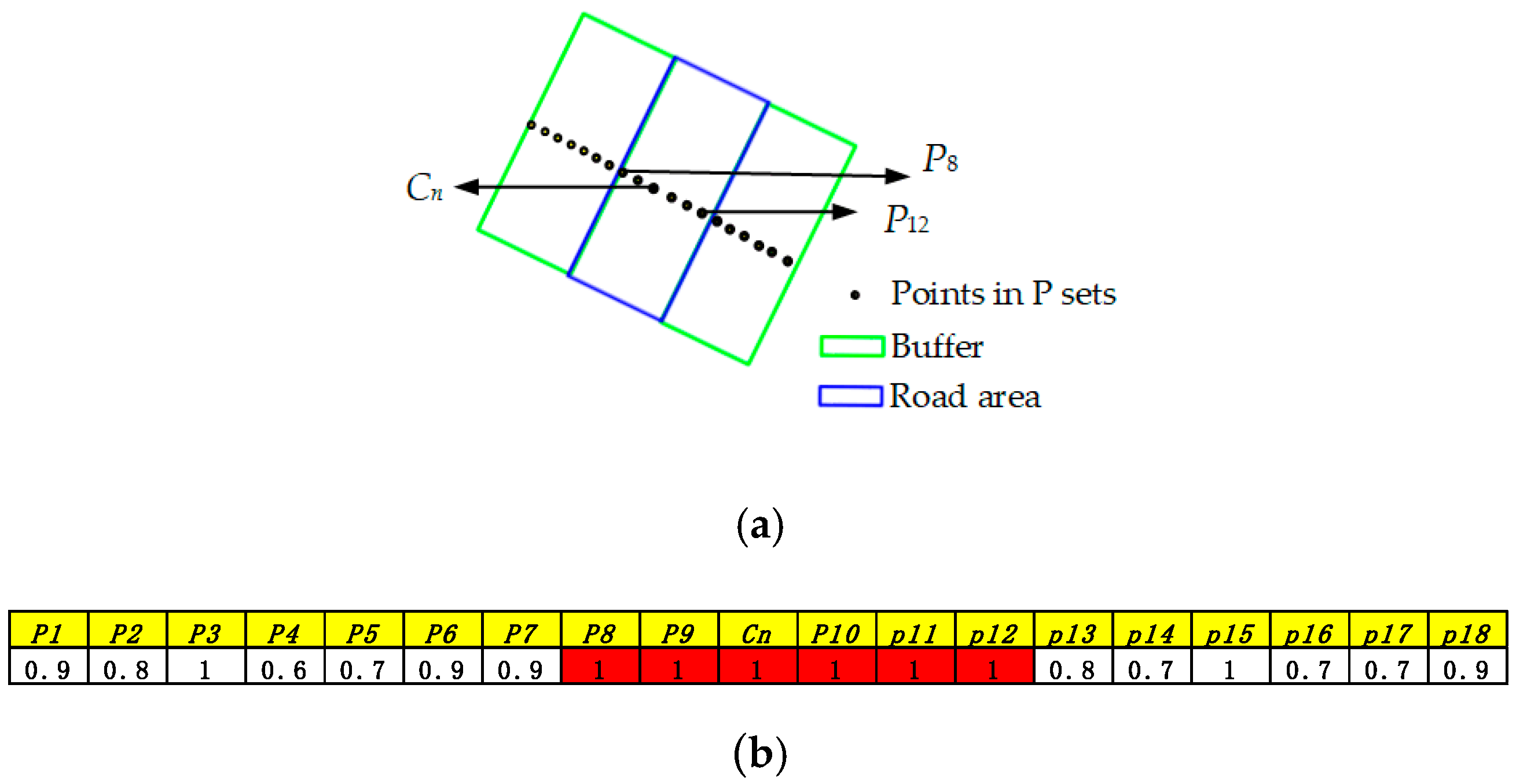
According to the characteristics of the high internal similarity of roads and the great difference between roads and backgrounds, the image value level of 0~255 is linearly compressed to the range of [0, 255/G] in the proposed method, where G is the magnitude unit. The magnitude unit G is shown in detail in the parameter settings of Section 3.2. As shown in Figure 8a, the texture self-similarity Rm between the different Pi template and the local road line Cn template is calculated as follows:
R m = 1 a b s ( ( s n s m ) / s m a x )
where sn is the ratio of the image mean value of the local road line to G, sm is the ratio of the image mean value of each template in the P set to G, and smax is the maximum value of the s difference between the local road line template and each template in the P set.
Figure 8b takes the local road line Cn as a reference, generates samples in sequence according to a distance of 2 pixels, and uses Equation (6) to search for the texture similarity value Rm from both sides to obtain the local road width of 12 pixels.
3.
Road width determination
The road image is partially disturbed by noise such as vehicles, and the local road width may have deviations; however, the entire road width is uniform. Therefore, probability statistics is carried out in the proposed method for all local widths of a road to determine the overall road width.
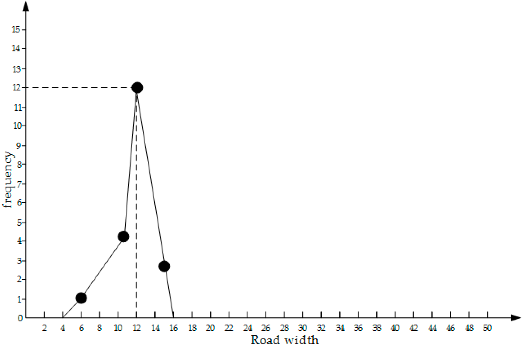
As shown in Figure 9, we constructed a histogram with the road width as the horizontal axis and the frequency as the vertical axis, and the statistical peak point is the road width W.
(2) Centerpoint autocorrection
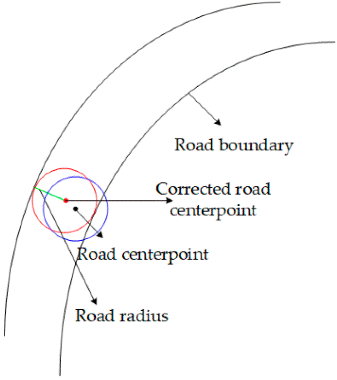
If a road line is located in the center of the road, based on the determined road width, road-positive samples can be accurately created by extending both sides of the road. When there is interference in the road, the extracted road line is might not coincide with the road centerline in the image, so it is necessary to extract the road centerline. Based on the determination of the road width, the circular template [43] method is used to update the position of the points on the road line. This method uses the gradient comparison of the circular template of the current point and the neighborhood points to complete the calculation of the road centerpoint and the road width. However, in our method, the road width was determined in the early stage, and we thus use the circular template with a fixed width to update the position. As shown in Figure 10, the green line is the determined road width, the red and blue circles are the correction templates, the black points are the points on the original road line, and the red points are the points on the road line after correction.
(3) Road-positive sample creation
By starting from the road centerline, and searching both sides with half the road width, the road-positive sample can be created. However, the corrected centerpoints may still contain inaccurate points. To solve this problem, the RANSAC algorithm [44] is used in the proposed method to fit the road centerpoints that have been obtained to form a more accurate road centerline:
Y = a x 2 + b x + c
where a, b, and c are parabolic parameters.
Equation (7) is the parabola road line fitting model selected in the proposed method. The RANSAC model is used to calculate three points each time to determine the parameters. By setting the sampling times as 1000, the maximum points in accordance with Formula (7) are selected to determine the parabola parameters and the beginning and ending points of the parabola are determined by the projection of two ends of the OSM vector line on a road cross section. Accordingly, a more accurate road centerline is obtained.

3. Experimental Analysis and Evaluation

3.1. Comparison Method

The deep learning method is the focus of road extraction. To verify the effectiveness of our method, we compared it with the deep learning method and used U Net [13] and CNN [38]. The residual U-shaped network [13] is based on the U-shaped network. Adding the residual module increases the depth of the network without changing the image resolution; the end-to-end road extraction target is achieved by using the jump structure. An improved CNN structure based on the road [38] first uses the first 13 convolution layers of VGG [45] to extract the levels instead of the manual features in previous road extraction methods. Secondly, three additional convolution layers are used to adapt to the road structure. Then, a deconvolution and fusion layer are combined, and a cross entropy loss function with road structure constraints is proposed. In the parameter setting, the number of network iterations is set to 30. The specific experimental settings are shown in Table 1.

3.2. Parameter Analysis

The proposed method sets six parameters, which are the angle constraint threshold σ, the magnitude unit γ, the scale factor λ, the constraint threshold of image value η, the constraint threshold δ, and the magnitude unit G. The reason for setting these parameters is discussed in this section.
(1) Angle constraint threshold σ.
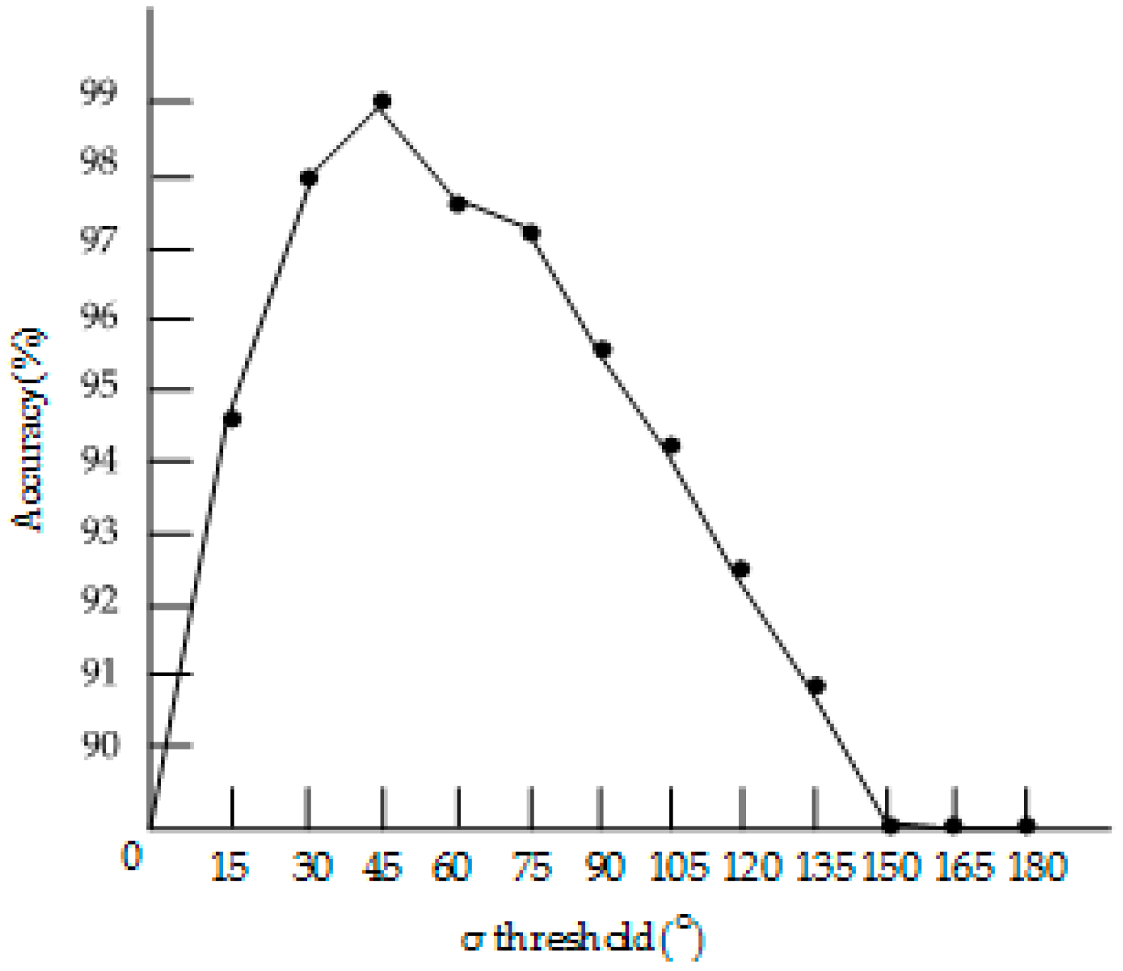
Considering the result of the line segment extraction in the image, it includes not only the edge of the road-related features but also the edges of the buildings perpendicular to the road direction. To reduce the interference, the angle constraint threshold σ is set. To obtain the best threshold, the threshold analysis chart is drawn with the angle constraint threshold as the horizontal axis and the local road directional accuracy as the vertical axis. As shown in Figure 11, when σ is 45°, the accuracy is the highest. Therefore, σ is set as 45° in this article.
(2) Magnitude unit γ.
In the local road line, the road direction usually changes little, so the magnitude unit γ is set as 15 in this article.
(3) Scale factor λ.
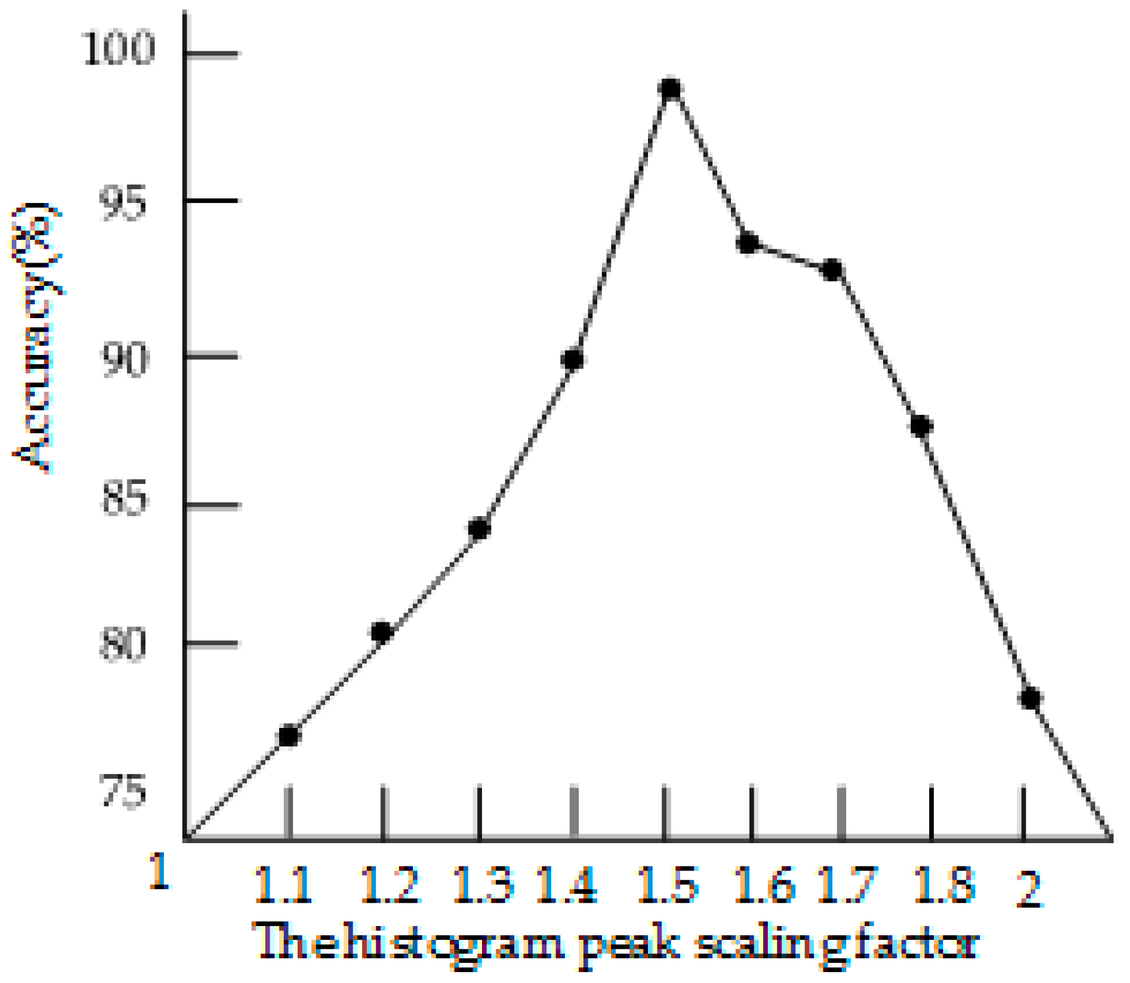
This parameter mainly highlights the relationship between the peak value of the line segment and the local road direction. If the value of λ is too small, it is easy to extract the wrong local road direction in the case of multiple peaks; if the value of λ is too large, it will lead to the problem of difficulty to predict the local road direction. Therefore, as shown in Figure 12, the local road direction accuracy obtained under different λ conditions is analyzed in this article, from which it can be determined that the local road direction accuracy is the highest when λ is 1.5.
(4) Constraint threshold of the image value η.
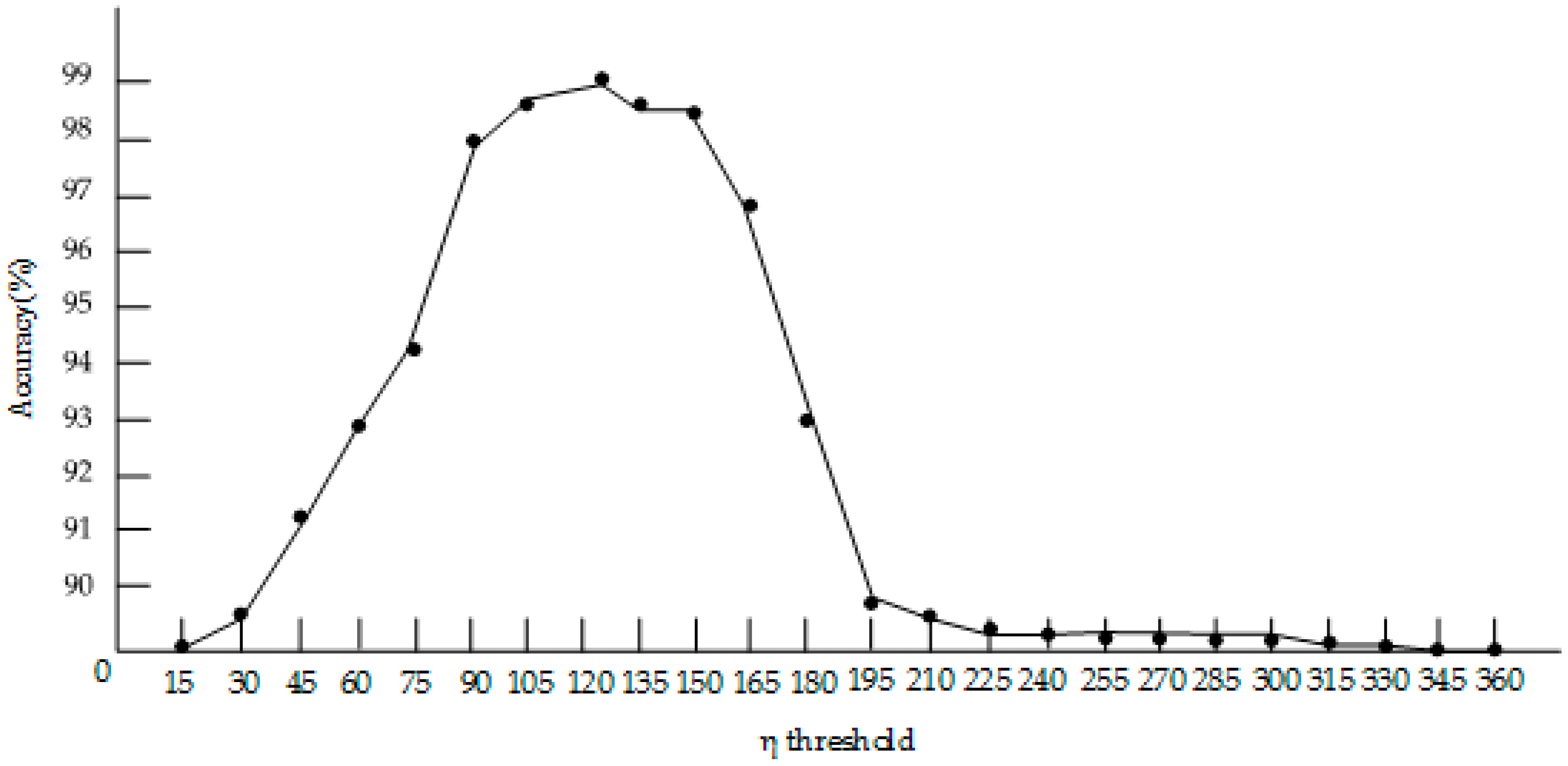
This parameter mainly considers the determination of candidate local road lines under the condition of road interference. To highlight the difference between the different candidate local road lines, the local road line extraction accuracy obtained under different η conditions is analyzed in this article. As shown in Figure 13, when the constraint threshold of the image value of η is 125, the accuracy of the local road line is the highest. Therefore, the constraint threshold of image value η is set to 125 in the proposed method.
(5) Constraint threshold δ.
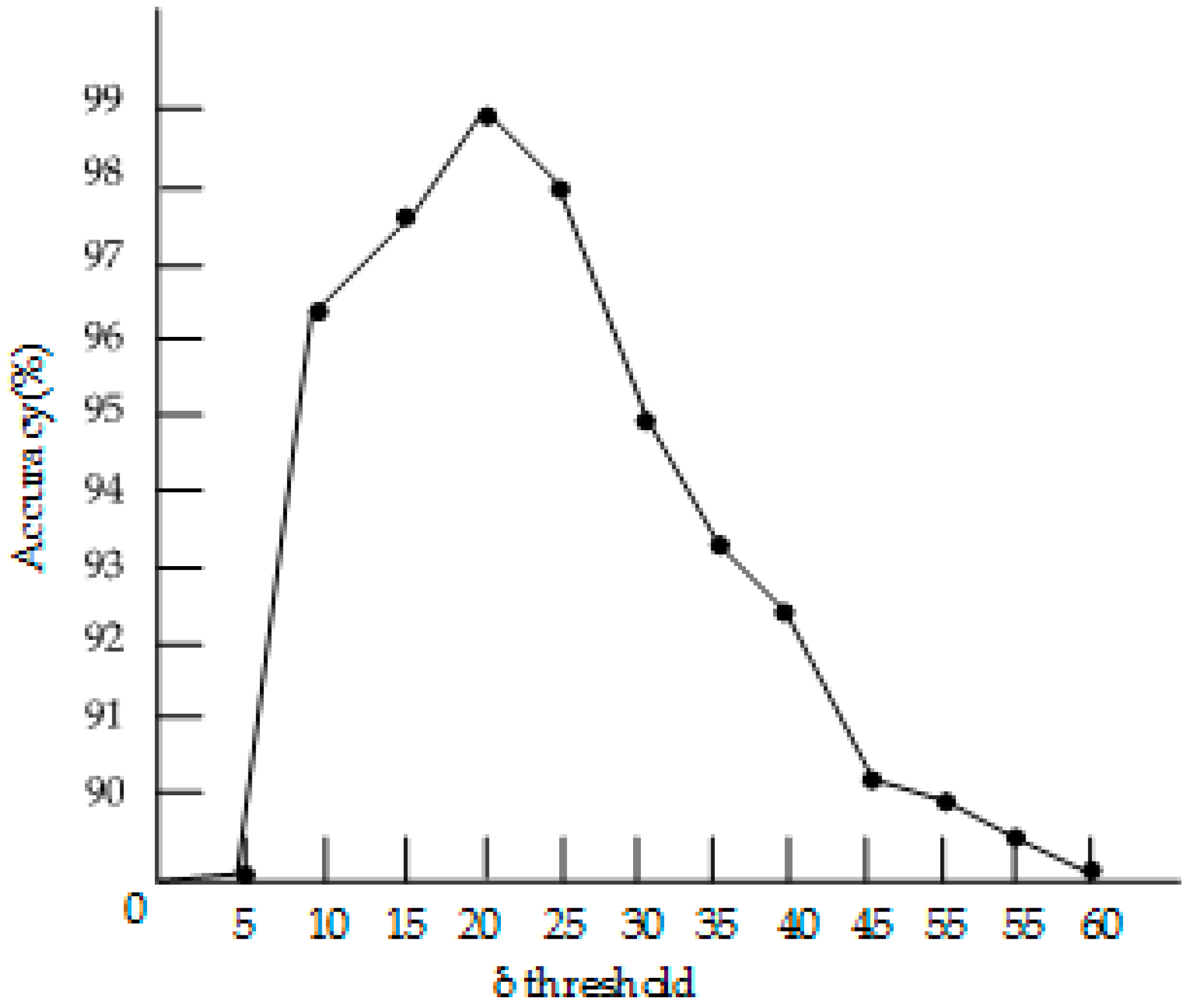
The threshold is mainly used to judge whether the candidate local road line is an effective local road line. If it is set too low, it is easy to exclude the correct local road line. If it is set too high, it is easy to reduce the accuracy of the local road line extraction. As shown in Figure 14, the local road line accuracy obtained under the different δ conditions was analyzed and thus δ was set to 20.
(6) Magnitude unit G.
Due to the influence of noise, the homogeneity of the road texture is bound to decline. If the setting of G is too small, the homogeneity of the road texture cannot be reflected. If G is too large, the non-road line may be mistaken for the road. Thus, G is set as 15 in this article.

3.3. Evaluation Index

To evaluate the effect of the extraction method in this article, three quantitative evaluation indexes were selected, namely, the integrity rate, accuracy rate, and extraction quality [46]. The calculation formulas of the three evaluation methods are as follows:
Integrity rate:
Com = C / ( C + N )
Accuracy rate:
Cor = C / ( C + I )
Extraction quality:
Q = C / ( C + N + I )
Among them, C is the total area of the correctly extracted road-positive samples, I is the total area of incorrectly extracted road-positive samples, and N is the total area of the unextracted road-positive samples.

3.4. Experimental Results and Analysis

3.4.1. Experiment 1

As shown in Figure 15, there is a certain position deviation after the OSM data were superimposed onto the orthophoto. We compare the proposed method with other methods. As shown in Figure 15, the CNN model and UNet model do not achieve a good extraction effect for most types of road, and there are road over-extraction and fracture phenomena. Especially for the road line with tree occlusion shown in the CNN model’s local view in Figure 15e, there are errors in the road extraction, which are caused by the deep learning mechanism. Similarly, as shown in the local enlarged view of the UNet model in Figure 15, the road extraction that uses the UNet model fails to show a good extraction effect, and some non-road areas are incorrectly extracted, which does not meet the standard of road-positive samples. Moreover, due to the shadow occlusion phenomenon on the road, the method does not have great anti-noise ability, and the occluded road line is broken, which has not been extracted completely and accurately. Compared with the two models, the experimental results of the method proposed in this article have the characteristics of high accuracy, which can be clearly shown in the local view of the proposed method in Figure 15. For the road with less noise and occlusion shown in the local view in Figure 15b–d, the proposed method can complete the creation of positive road samples. However, for large occlusion areas, as shown in Figure 15e, the proposed method can still guarantee the connectivity of the roads. The method proposed in this article is effective for road intersections, road bends and road lines shaded by vehicles and trees, and the quality advantage of the extraction is obvious. However, the CNN model and UNet model cannot extract roads well, especially the CNN model, which is unsuitable for creating road-positive samples.

3.4.2. Experiment 2

The local views of Figure 16a–e show the presence of vehicle noise, edge blur, a large curvature change, and tree shadow occlusion in the road. To verify the proposed method, we show the results of each step.
As shown in Figure 16, the blue line is the OSM vector line. From the local view, we can see that there is a deviation between the road direction provided by the OSM and the road direction in the image. This problem will increase the difficulty of the subsequent road line extraction. Therefore, this article introduces the results of the line segment extraction and creates the LSOH model to adjust the direction of the OSM to determine the local road direction. As shown in Figure 16, in the local road direction determination step, the violet line is the corrected OSM vector line. It can be seen that the corrected OSM vector line can more accurately indicate the local road direction.
Based on the local road direction determination, the road homogeneity constraint, road texture feature statistical model, and local road line set determination were used to extract the local road line set in some areas, as shown in the local road line set steps in Figure 16b,c. However, it is also found that when the road has an occlusion problem, as shown in Figure 16d,e, the local road line in this area is not extracted, and road line fracture occurs. To solve this problem, this article uses the iterative interpolation algorithm to take the endpoints of the local road lines on both sides obtained earlier as seed points and searches for the optimal seed points on the vertical line. As shown in the local view of the road lines in Figure 16d,e, the road lines at the fracture are connected.
According to the visual analysis of the results of road line extraction in Figure 16, it can be seen that, although the road line is inside the road, it is not necessarily in the central area of the road. Therefore, this article creates the LTSS model to obtain the road width. Based on the determination of the road width, the centerpoint autocorrection model is established, and the RANSAC algorithm is used for fitting to obtain the road centerline. At the same time, the road-positive sample is created by combining the road width. As shown in Figure 16, the road-positive sample has been extracted. This indicates that the method is effective for complex rural roads with noise, fuzzy road edges, shadow shading, and large curvature variation.

3.4.3. Experiment 3

As shown in Figure 17, the isolation belt is set in the middle of the local road, and there are high levels of tree shadows and vehicle noise. The greatest difficulty lies in the fact that the local road has a two-way lane, which leads to the poor texture homogeneity of the road, and greatly increases the difficulty of road-positive sample creation. However, through the positive sample creation results in Figure 17, it can be found that the method proposed in this article is still effective for road lines with shadows, noise, and isolation bands. Due to the large amount of noise at the edge of the road, the obtained local road width is generally slightly smaller than the real local road width, which results in the statistical road width being less than the real road width, and leads to the incomplete extraction of the road-positive samples. However, considering the complexity of the image and compared with the ground truth, we can determine that the method proposed in this article still shows a good level of accuracy.

3.4.4. Experimental Analysis

Most road samples are produced manually, and no study has provided samples for deep learning by using traditional methods. Deep learning methods have strong generalizability, and the accuracy of automatic extraction is widely recognized. Therefore, to fully verify the effectiveness of the method proposed in this article, we compare the artificial road-positive sample method and two deep learning network methods [13,38] with the proposed method.
The results of the three groups of experiments (Figure 15, Figure 16 and Figure 17) and the ground truthing show that the proposed method has good effects for road-positive sample creation. However, according to the result map of the deep learning method shown in Experiment 1, the road extraction results are not very satisfactory; there are a lot of over-extraction or under-extraction phenomena, and the extraction effects for the shadow occlusion in the image are poor (Figure 15 CNN and UNet results). The specific data are shown in Table 2. In terms of the integrity rate, accuracy rate, and extraction quality, the UNet network and CNN network are lower than the proposed method. This is because deep learning is a supervised learning method. In the process of network training, the network parameters are updated by iterating the network training based on the existing samples, so that the network model can effectively extract and represent the deep features and complete the complex feature mapping task. Therefore, the number, quality, type of samples, and training model will impact the results, which makes the performance of a network model limited and fails to fully reflect the advantages of the deep learning method. Therefore, it is necessary to create multi-regions and different types of road samples automatically. The method proposed in this article can effectively solve the problems of shadow and tree occlusion and create road-positive samples with good extraction quality. Furthermore, as shown in Table 2, the total training and prediction time of the CNN network and U Net network were 366 min and 352 min, respectively.
To verify the effectiveness of this method, the integrity rate, accuracy rate, and extraction quality were used to evaluate the road-positive samples. As shown in Table 3, the results of the experiments show that the extraction results of the proposed method suggest high integrity. Although Experiment 3 is greatly disturbed by noise, the integrity and extraction quality still reach approximately 85%. Moreover, the three experiments took different times, among which Experiment 1 took the longest time but was still within 10 min. This result is mainly due to the different coverage types and noise types of the three groups of data. In Experiment 1, the image coverage area is Hobart City, Australia. The OSM integrity is high, the image resolution is high, the road boundary is obvious, and the noise is less. Therefore, the extraction integrity, accuracy, and extraction quality are high in the experiment. In Experiment 2, the image covers rural areas, and the population density affects the integrity of the OSM data. The data in densely populated areas are more complete than the data in sparsely populated areas [47]. The image coverage area has a low population density, and only a few main roads have OSM data. The roads in the image with corresponding OSM data are analyzed in this article, where the number of roads is relatively small, and a small number of local error corrections directly reduces the accuracy of the extraction results; therefore, the accuracy is the lowest in Experiment 2 among the three experiments. In Experiment 3, the area covered by the image is suburban, densely populated, and the scene is complex. There is a lot of vehicle noise at the edge of the road, and the situation is complex and changeable. The road width determined by this method is smaller than the road width in the image, which results in a low integrity and relatively low extraction quality.

4. Discussion

To provide reliable road-positive samples for deep learning, the following four aspects are studied in this article: considering the non-overlapping phenomenon between the OSM direction and the local road direction in the image, the local road direction is determined by using the LSOH model; the local road line set is obtained by using the road homogeneity constraint rule, road texture feature statistical model, and local road line set extraction; the road line with an iterative interpolation algorithm is connected for the road line fracture; and an LTSS model is created to determine road width, the road centerline is obtained by using the centerpoint autocorrection model and the RANSAC algorithm, and the road-positive sample is created using the road width and road centerline. The specific significance of this work is as follows:
(1)
Effective connection between traditional methods and deep learning methods.
Traditional deep learning is dependent on samples mainly produced manually. To solve the problem of insufficient samples, we usually expand the samples on the basis of existing samples, but experiments show that the method of sample expansion does not have strong migration [48]. Thus, the creation of samples remains an obstacle that restricts the application of deep learning. Compared with the deep learning method, the proposed method in this article is a traditional method. The purpose of this method is to create road-positive samples automatically; that is, a process from 0 to 1, which aims to achieve the automatic creation of positive road samples, and provides basic samples for the application of deep learning. This method therefore offers an effective connection between the traditional method and the deep learning method.
(2)
Enhancement of the universality of the deep learning method.
The deep learning method is limited by the number and type of samples, and it is difficult to transfer different sample data. On the one hand, it increases the demand of sample production, but on the other hand, it reduces the scope of the application of the deep learning method. The proposed method in this article is based on OSM data to create road positive-samples and can form a variety of road-positive samples under different interference conditions, such as occlusion, trees, and vehicles. As a result, the pressure of sample creation is reduced, and an effective guarantee for the application of the deep learning method is obtained.

5. Conclusions

Based on prior information provided by the OSM data, we propose a method for creating road-positive samples. To solve the problem of divergence between the direction indicated by OSM data and the local road direction in the image, we make full use of the image line segment to obtain the local road direction, which is convenient for subsequent road line extraction. The local road line set is extracted by the road homogeneity constraint rule, road texture feature statistical model, and local road line set extraction. The problem of road line fracture is solved by using an iterative interpolation algorithm. An LTSS model is established to obtain the road width. A centerpoint autocorrection model and the RANSAC algorithm are used to solve the problem of the inaccurate location of the road line, and the road centerline is obtained. Based on the road width and road centerline, the road-positive sample creation is completed. Through the analysis of three groups of different types of experimental data, the effectiveness of the algorithm is verified. In addition, we compare the results of the road-positive sample creation with those of artificial production and the deep network learning method. The experimental results show that the proposed method can effectively create road-positive samples under interference from vehicles, trees, and local shadows with a high extraction accuracy of approximately 97%. However, the proposed method in this article still has shortcomings. For example, the template is used to find the centerpoint pixel-by-pixel, and the parameter setting usually depends on the statistical results of the data set, which will affect the timeliness and generalization ability of the method. In addition, the premise of creating road-positive samples in this article is that the road is clear and the interference is relatively small; it is not suitable for images with noise accounting for more than 20% of the total road area or without corresponding OSM data. We will further improve the robustness, generalization, and timeliness of the method in future studies.

Author Contributions

Conceptualization, C.L.; funding acquisition, J.D.; methodology, J.D.; project administration, Y.Z.; resources, H.A.; writing—original draft, C.L.; writing—review and editing, C.L. All authors have read and agreed to the published version of the manuscript.

Funding

This research was funded by The National Natural Science Foundation of China (42071428); The National Natural Science Foundation of China (420713743); the Key Laboratory of Land Satellite Remote Sensing Application Center, Ministry of Natural Resources of the People’s Republic of China (KLSMNR-202004); Liaoning Provincial Department of Education Project Services Local Project under Grant (LJ2019FL008); Beijing Key Laboratory of Urban Spatial Information Engineering (2020221); Key Laboratory for National Geography State Monitoring (National Administration of Surveying, Mapping and Geoinformation) (2018NGCM01); Key Laboratory of Surveying and Mapping Science and Geospatial Information Technology of Ministry of Natural Resources (2020-3-5).

Acknowledgments

The authors wish to thank the editors and reviewers.

Conflicts of Interest

The authors declare no conflict of interest.

References

  1. Ziemsa, M.; Gerkeb, M.; Heipke, C. Automatic road extraction from remote sensing imagery incorporating prior information and colour segmentation. Remote Sens. Spat. Inf. Sci. 2007, 36, 141–147. [Google Scholar]
  2. Huang, X.; Lu, Q.; Zhang, L. A multi-index learning approach for classification of high-resolution remotely sensed images over urban area. ISPRS J. Photogramm. Remote Sens. 2014, 90, 36–48. [Google Scholar] [CrossRef]
  3. Steger, C.; Glock, C.; Eckstein, W. Model-based road extraction from images. In Automatic Extraction of Man-Made Objects from Aerial and Space Images; Birkhäuser: Basel, Switzerland, 1995. [Google Scholar]
  4. Baumgartner, A.; Steger, C.T.; Mayer, H.; Eckstein, W. Semantic objects and context for finding roads. Proc. SPIE Int. Soc. Opt. Eng. 1997, 3072, 98–109. [Google Scholar]
  5. Treash, K.; Amaratunga, K. Automatic road detection in grayscale aerial images. J. Comput. Civ. Eng. 2000, 14, 60–69. [Google Scholar] [CrossRef] [Green Version]
  6. Sghaier, M.O.; Lepage, R. Road extraction from very high resolution remote sensing optical images based on texture analysis and beamlet transform. IEEE J. Sel. Top. Appl. Earth Obs. Remote Sens. 2016, 9, 1946–1958. [Google Scholar] [CrossRef]
  7. Shao, Y.; Guo, B.; Hu, X.; Di, L. Application of a fast linear feature detector to road extraction from remotely sensed imagery. IEEE J. Sel. Top. Appl. Earth Obs. Remote Sens. 2010, 4, 626–631. [Google Scholar] [CrossRef]
  8. Talbot, H.; Appleton, B. Efficient complete and incomplete path openings and closings. Image Vis. Comput. 2007, 25, 416–425. [Google Scholar] [CrossRef]
  9. Kass, M.; Witkin, A.; Terzopoulos, D. Snakes: Active contour models. Int. J. Comput. Vis. 1988, 1, 321–331. [Google Scholar] [CrossRef]
  10. Blaschke, T.; Hay, G.; Kelly, M.; Lang, S.; Hofmann, P.; Addink, E.; Feitosa, R.; Meer, F.; Werff, H.; Coillie, F.; et al. Geographic object-based image analysis—Towards a new paradigm. ISPRS J. Photogramm. Remote Sens. 2014, 87, 180–191. [Google Scholar] [CrossRef] [Green Version]
  11. Alshehhi, R.; Marpu, P.R. Hierarchical graph-based segmentation for extracting road networks from high-resolution satellite images. ISPRS J. Photogramm. Remote Sens. 2017, 126, 245–260. [Google Scholar] [CrossRef]
  12. Cheng, G.; Zhou, P.; Han, J. RIFD-CNN: Rotation-invariant and fisher discriminative convolutional neural networks for object detection. In Proceedings of the IEEE Conference on Computer Vision and Pattern Recognition (CVPR), Las Vegas, NV, USA, 27–30 June 2016; pp. 2884–2893. [Google Scholar]
  13. Zhang, Z.; Liu, Q.; Wang, Y. Road extraction by deep residual U-Net. IEEE Geosci. Remote Sens. Lett. 2017, 99, 1–5. [Google Scholar] [CrossRef] [Green Version]
  14. Liu, R.; Miao, Q.; Song, J.; Quan, Y.; Li, Y.; Xu, P.; Dai, J. Multiscale road centerlines extraction from high-resolution aerial imagery. Neurocomputing 2019, 329, 384–396. [Google Scholar] [CrossRef]
  15. Gong, J.; Ji, S. Photogrammetry and deep learning. Acta Geod. Cartogr. Sin. 2018, 47, 693–704. [Google Scholar]
  16. Teerapong, P.; Kulsawasd, J.; Siam, L.; Panu, S. Road segmentation of remotely-sensed images using deep convolutional neural networks with landscape metrics and conditional random fields. Remote Sens. 2017, 9, 680–698. [Google Scholar]
  17. Xu, Y.; Xie, Z.; Feng, Y.; Chen, Z. Road extraction from high-resolution remote sensing imagery using deep learning. Remote Sens. 2018, 10, 1461. [Google Scholar] [CrossRef] [Green Version]
  18. Ding, G.; Guo, Y.; Chen, K. DECODE: Deep confidence network for robust image classification. IEEE Trans. Image Process. 2019, 28, 3752–3765. [Google Scholar] [CrossRef] [PubMed] [Green Version]
  19. Gao, L.; Zhang, X.; Gao, J. Fusion image based radar signal feature extraction and modulation recognition. IEEE Access 2019, 7, 13135–13148. [Google Scholar] [CrossRef]
  20. Gui, Y.-M.; Wang, R.-J.; Wang, X.; Wei, Y.-Y. Using Deep Neural Networks to improve the performance of protein-protein interactions prediction. Int. J. Pattern Recognit. Artif. Intell. 2020. [Google Scholar] [CrossRef]
  21. Zhu, X.; Ghahramani, Z.; Lafferty, J. Semi-supervised learning using gaussian fields and harmonic functions. In Proceedings of the 20th International conference on Machine learning, Washington, DC, USA, 21–24 August 2003; pp. 912–919. [Google Scholar]
  22. Zhou, D.; Bousquet, O.; Lal, T.N. Learning with local and global consistency. Adv. Neural Inf. Process. Syst. 2004, 16, 321–328. [Google Scholar]
  23. Belkin, M.; Niyogi, P.; Sindhwani, V. Manifold regularization: A geometric framework for learning from labeled and unlabeled examples. J. Mach. Learn. Res. 2006, 7, 2399–2434. [Google Scholar]
  24. Miller, D.J.; Uyar, H.S. A mixture of experts classifier with learning based on both labeled and unlabeled data. Adv. Neural Inf. Process. Syst. 1997, 9, 571–577. [Google Scholar]
  25. Nigam, K.; Mc Callum, A.K.; Thrun, S. Text classification from labeled and unlabeled documents using EM. Mach. Learn. 2000, 39, 103–134. [Google Scholar] [CrossRef] [Green Version]
  26. Chapelle, O.; Zien, A. Semi-supervised learning by low density separation. In Proceedings of the Tenth International Workshop on Artificial Intelligence and Statistics, Bridgetown, Barbados, 6–8 January 2005; pp. 57–64. [Google Scholar]
  27. Li, Y.F.; Tsang, I.W.; Kwok, J.T. Convex and scalable weakly labeled. J. Mach. Learn. Res. 2013, 14, 2151–2188. [Google Scholar]
  28. Zhou, Z.H.; Li, M. Semi-supervised learning by disagreement. Knowl. Inf. Syst. 2010, 24, 415–439. [Google Scholar] [CrossRef]
  29. Blum, A.; Mitchell, T. Combining labeled and unlabeled data with co-training. In Proceedings of the Eleventh Annual Conference on Computational Learning Theory, Madison, WI, USA, 24–26 July 1998; pp. 92–100. [Google Scholar]
  30. Wan, T.; Lu, H.; Lu, Q.; Luo, N. Classification of high-resolution remote-sensing image using openstreetmap information. IEEE Geosci. Remote Sens. Lett. 2017, 14, 2305–2309. [Google Scholar] [CrossRef]
  31. Cao, C.; Sun, Y. Automatic road centerline extraction from imagery using road GPS data. Remote Sens. 2014, 6, 9014–9033. [Google Scholar] [CrossRef] [Green Version]
  32. Li, Q.; Luan, X.; Luan, X.; Yang, B.S.; Liu, L. Polygon-based approach for extracting multilane roads from openstreetmap urban road networks. Int. J. Geogr. Inf. Sci. 2014, 28, 2200–2219. [Google Scholar] [CrossRef]
  33. Chen, B.; Sun, W.; Vodacek, A. Improving image-based characterization of road junctions, widths, and connectivity by leveraging openstreetmap vector map. In Proceedings of the IEEE Geoscience and Remote Sensing Symposium, Quebec City, QC, Canada, 13–18 July 2014. [Google Scholar]
  34. Zhang, J.-l.; Zhang, X.-f.; Xu, D.; Wang, D.-s.; Liu, Q.-h.; Li, N. Road_net data construction for intelligent transportation based on the open street map. Road Traffic Saf. 2014, 1, 8. [Google Scholar]
  35. Haklay, M.; Weber, P. OpenStreetMap: User-generated street maps. IEEE Pervasive Comput. 2008, 7, 12–18. [Google Scholar] [CrossRef] [Green Version]
  36. Zhou, G.; Zhang, R.; Zhang, D.; Huang, J.; Baysal, O. Real-time ortho-rectification for remote-sensing images. Int. J. Remote Sens. 2018, 40, 2451–2465. [Google Scholar] [CrossRef]
  37. Neis, P.; Zipf, A. Analyzing the contributor activity of a volunteered geographic information project—The case of openstreetmap. ISPRS Int. J. Geo Inf. 2012, 1, 146–165. [Google Scholar] [CrossRef]
  38. Wei, Y.; Wang, Z.; Xu, M. Road structure refined CNN for road extraction in aerial image. IEEE Geosci. Remote Sens. Lett. 2017, 14, 709–713. [Google Scholar] [CrossRef]
  39. Jiguang, D.; Zhang, L.; Li, J.; Fang, X. A line extraction method for chain code tracking with phase verification. Acta Geod. Cartogr. Sin. 2017, 46, 218–227. [Google Scholar]
  40. Vosselman, G.; de Knech, J. Automatic Extraction of Manmade Objects from Aerial and Space Images; Birkhauser Verlag: Basel, Switzerland, 1995; pp. 65–74. [Google Scholar]
  41. Ballard, D.H. Generalizing the hough transform to detect arbitrary shapes. Pattern Recognit. 1981, 13, 111–122. [Google Scholar] [CrossRef]
  42. Lian, R.; Wang, W.; Li, J. Road extraction from high-resolution remote sensing images based on adaptive circular template and saliency map. Acta Geod. Cartogr. Sin. 2018, 47, 950–958. [Google Scholar]
  43. Tan, R.; Wan, Y.; Yuan, F. Semi-automatic road extraction of high resolution remote sensing images based on circular template. Bull. Surv. Mapp. 2014, 63–66. [Google Scholar]
  44. Fischler, M.A.; Bolles, R.C. Random Sample Consensus: A Paradigm for Model Fitting with Applications to Image Analysis and Automated Cartography. Commun. ACM 1981, 24, 381–395. [Google Scholar] [CrossRef]
  45. Simonyan, K.; Zisserman, A. Very deep convolutional networks for large-scale image recognition. arXiv 2014, arXiv:1409.1556. [Google Scholar]
  46. Sujatha, C.; Selvathi, D. Connected component-based technique for automatic extraction of road centerline in high resolution satellite images. EURASIP J. Image Video Process. 2015, 2015, 8. [Google Scholar] [CrossRef] [Green Version]
  47. Arsanjani, J.J.; Zipf, A.; Mooney, P.; Helbich, M. Introduction to OpenStreetMap in GIScience: Experiences, research, and applications. In OpenStreetMap in GIScience. Lecture Notes in Geoinformation and Cartography; Springer: Cham, Switzerland, 2015; p. 15. [Google Scholar]
  48. Gao, K.; Zhang, Y.; Zhang, W.; Lin, S. Affine stable characteristic based sample expansion for object detection. In Proceedings of the 9th ACM International Conference on Image and Video Retrieval, CIVR 2010, Xi’an, China, 5–7 July 2010. [Google Scholar]
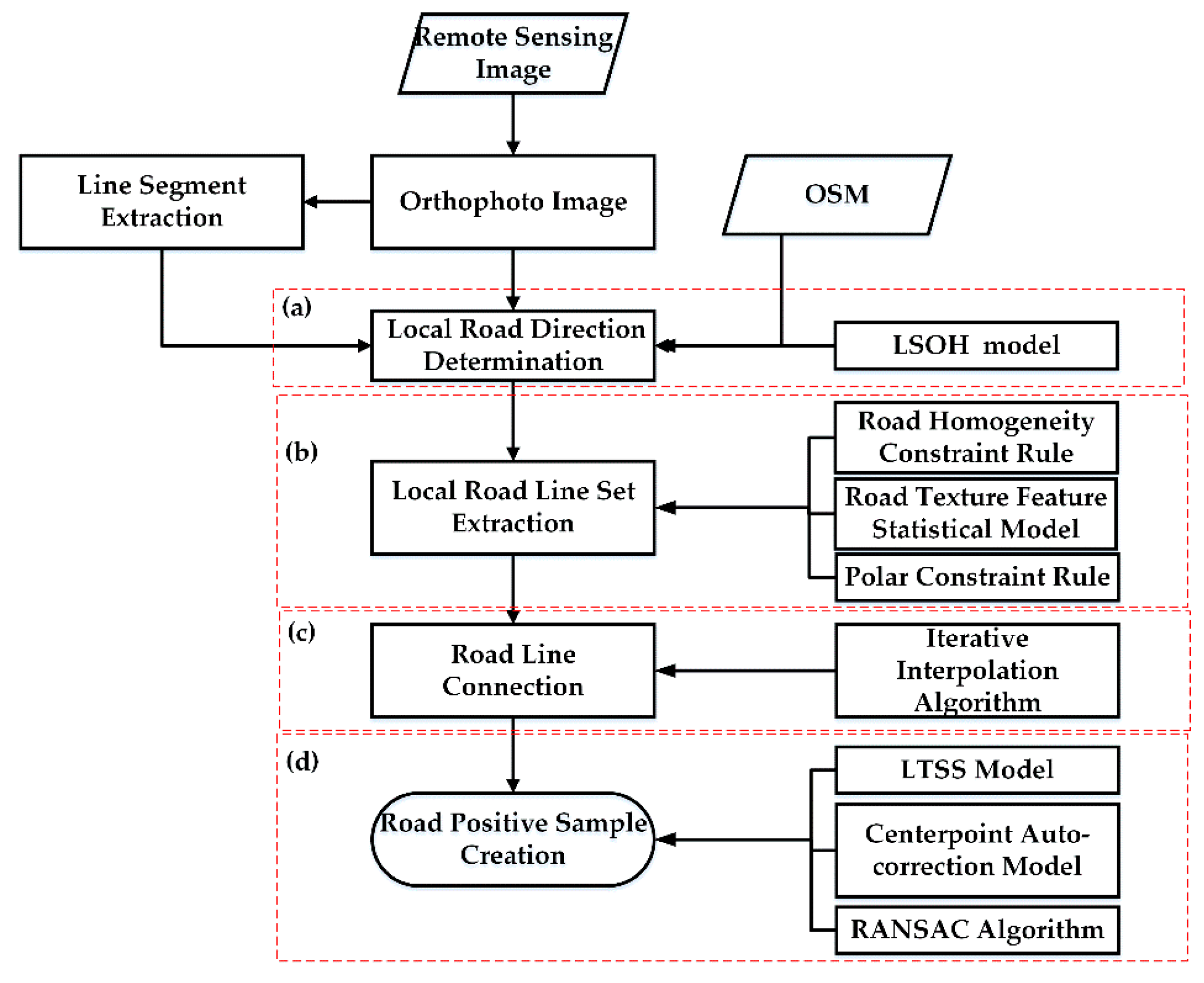
Figure 1. Method flowchart.
Remotesensing 12 03612 g001
Figure 2. Local road direction determination: (a) the overlay of OSM data and the line segment extraction results with the image and a locally enlarged image; (b) the LSOH model.
Remotesensing 12 03612 g002
Figure 3. Road homogeneity constraint.
Remotesensing 12 03612 g003
Figure 4. Road texture feature statistical model.
Remotesensing 12 03612 g004
Figure 5. Local road line set optimization.
Remotesensing 12 03612 g005
Figure 6. Road line connection.
Remotesensing 12 03612 g006
Figure 7. Statistical region construction.
Remotesensing 12 03612 g007
Figure 8. Local texture self-similarity analysis.
Remotesensing 12 03612 g008
Figure 9. Probability statistics of road width.
Remotesensing 12 03612 g009
Figure 10. Centerpoint autocorrection.
Remotesensing 12 03612 g010
Figure 11. Setting of the angle constraint threshold σ.
Remotesensing 12 03612 g011
Figure 12. Setting of the scale factor λ.
Remotesensing 12 03612 g012
Figure 13. Setting of the constraint threshold of image value η.
Remotesensing 12 03612 g013
Figure 14. Setting of the constraint threshold δ.
Remotesensing 12 03612 g014
Figure 15. Effect picture of Experiment 1 and its local enlarged view; (a) OSM data; (bd) the road with less noise and occlusion; (e) large occlusion areas
Remotesensing 12 03612 g015
Figure 16. Partial display of the effect of the different steps; (ae) the presence of vehicle noise, edge blur, a large curvature change, and tree shadow occlusion in the road.
Remotesensing 12 03612 g016
Figure 17. Effect picture of Experiment 3 and its local enlarged view (ae).
Remotesensing 12 03612 g017
Table 1. Comparison method parameter setting table.
CNNUNet
Network layer3757
Convolution kernel size3
Pool size2 * 2
Paddingsame
Activation functionReLU
Optimization functionAdam
Losscategorical_crossentropy
Table 2. Results of the different methods.
MethodCom %Cor %Q %Time (min)
The proposed method96.5897.0893.859
CNN network71.3489.5168.85366
UNet network81.2586.5780.79352
Table 3. Results of the proposed method.
ExperimentCom %Cor %Q %Time (min)
Experiment 294.2197.0291.564
Experiment 385.2297.7183.557
Publisher’s Note: MDPI stays neutral with regard to jurisdictional claims in published maps and institutional affiliations.