Multi-Temporal Predictive Modelling of Sorghum Biomass Using UAV-Based Hyperspectral and LiDAR Data

Abstract

High-throughput phenotyping using high spatial, spectral, and temporal resolution remote sensing (RS) data has become a critical part of the plant breeding chain focused on reducing the time and cost of the selection process for the “best” genotypes with respect to the trait(s) of interest. In this paper, the potential of accurate and reliable sorghum biomass prediction using visible and near infrared (VNIR) and short-wave infrared (SWIR) hyperspectral data as well as light detection and ranging (LiDAR) data acquired by sensors mounted on UAV platforms is investigated. Predictive models are developed using classical regression-based machine learning methods for nine experiments conducted during the 2017 and 2018 growing seasons at the Agronomy Center for Research and Education (ACRE) at Purdue University, Indiana, USA. The impact of the regression method, data source, timing of RS and field-based biomass reference data acquisition, and the number of samples on the prediction results are investigated. R² values for end-of-season biomass ranged from 0.64 to 0.89 for different experiments when features from all the data sources were included. Geometry-based features derived from the LiDAR point cloud to characterize plant structure and chemistry-based features extracted from hyperspectral data provided the most accurate predictions. Evaluation of the impact of the time of data acquisition during the growing season on the prediction results indicated that although the most accurate and reliable predictions of final biomass were achieved using remotely sensed data from mid-season to end-of-season, predictions in mid-season provided adequate results to differentiate between promising varieties for selection. The analysis of variance (ANOVA) of the accuracies of the predictive models showed that both the data source and regression method are important factors for a reliable prediction; however, the data source was more important with 69% significance, versus 28% significance for the regression method.

1. Introduction

Biomass yield is an important trait of biofuel crops such as sorghum, as it is a key factor in determining the amount of biofuel that can be produced. With recent advances in science and technology surrounding genotyping, it has become possible to create numerous genotypes of a plant [1] and then select the genotypes with the maximum biomass production. However, traditional methods of biomass measurement involving labor-intensive and time-consuming destructive sampling do not meet the requirements for timely evaluation of the genotypes in large-scale breeding programs. Recently, remote sensing (RS) data have been explored for estimation of many phenotypic traits, including leaf area index (LAI) [2,3], canopy height [4,5], nitrogen content [6], and biomass [7,8,9,10,11], to replace traditional in-field phenotyping.

Sensors on satellites and manned aircraft can provide data with high spectral resolution, but the spatial and temporal resolutions are inadequate for agricultural breeding programs that are based on small plots. Remote sensing via unmanned aerial vehicles (UAV) is currently being investigated as a means to close the gap because of its capability to acquire the high temporal and spatial resolution data required for high throughput phenotyping over relatively limited areas. UAVs can collect huge quantities of data “on demand”, providing opportunities for estimation and prediction of a wide range of agronomic traits [12,13,14,15,16,17,18,19,20,21,22,23,24].

In this study, remotely sensed biomass prediction of varieties of sorghum is investigated using the data acquired by RGB, hyperspectral and LiDAR sensors mounted on UAV platforms. Sorghum has attracted attention in recent years, both for its broad-based potential usage and its drought and heat tolerance. The grain of some varieties is now used for human consumption and animal feed in developed, as well as developing countries. Recently, some varieties of sorghum have been developed as an energy crop that can produce reasonable quantities of ethanol [25]. Sorghum has an annual growth cycle, high calorific value, and low management cost [25], making it an efficient biofuel crop. Many studies focus on developing enhanced genotypes that can produce more energy-rich plant material (biomass) [26]. It is important for these breeding studies to predict the end-of-season yield biomass of the planted varieties as soon as possible in the growing season to screen varieties, and thus reduce investment of expensive resources in monitoring for the whole season.

Biomass prediction based on data analytics models and RS data is challenging for multiple reasons, including (1) the complex relationship between biomass and RS data [27], (2) limited number of ground reference samples for developing and validating models for an experiment [28], and (3) high variability between the samples in an experiment [29]. Moreover, the relationships between the RS-based features and traits vary across the growing season [27]. Extraction of robust, explanatory features as predictors of the trait of interest is critical to development of machine learning models. A small number of field reference samples relative to the number of features (and thereby potentially the number of parameters to estimate) is a difficult issue for remote sensing-based phenotyping. Unfortunately, reference sampling data is time-consuming and expensive to collect in agricultural fields.

In this study, the objective is to develop baseline predictive models for sorghum biomass yield based on classical machine learning methods using multi-date remote sensing and ground reference data. The impact of timing of the data acquisition relative to days since sowing and the importance of the features extracted from the data are also investigated.

The remainder of this paper is organized as follows. Section 2 surveys the literature on the predictive models based on remote sensing data. In Section 3, the study area, reference data, and remote sensing data are described. Additionally, the methodologies including feature extraction, regression models, as well as statistical analysis are explained. Experimental results are presented in Section 4 and discussed in Section 5, and finally, conclusions are drawn in Section 6.

2. Related Work

Many studies have explored the potential for prediction or estimation of phenotypic traits utilizing spectral data. Potgieter et al. [2] found that indices obtained from a UAV-based multispectral sensor over a sorghum field with two different genotypes were correlated with the LAI measured in the field. Using spectrometer measurements acquired in wheat fields in different locations at multiple times during three growing seasons, Feng et al. [30] demonstrated that the nitrogen content of the leaves are highly correlated with the parameters derived from the first derivative of reflectance. The authors investigated correlation between phenotypic traits and remote sensing-based features. Estimation of the values of quantitative traits such as biomass at a given date, or prediction at a future date based on earlier data are more difficult.

Researchers have developed predictive models based on various remote sensing inputs and modeling approaches. Foster et al. [31] compared the performance of partial least squares regression (PLSR) and linear regression models in estimating biomass of a high-biomass sorghum variety. They concluded that PLSR can provide more accurate predictions using the normalized difference vegetation index (NDVI) calculated from field spectrometer measurements collected in July (three months after sowing). Yue et al. [32] also demonstrated that the PLSR provided the best results among the eight regression techniques investigated for wheat biomass estimation. Fassnacht et al. [33] investigated the importance of the prediction method, as well as sample size and sensor type for biomass predictions in forest environments, with the best results being obtained with a random forest (RF) model. Using airborne LiDAR and spaceborne hyperspectral data, the authors concluded that for their experiments, the sensor type was the most important factor in the prediction accuracy.

Multiple studies have also investigated biomass prediction using LiDAR data [8,34,35,36,37,38,39,40,41,42,43]. Harkel et al. [35] evaluated the accuracy of biomass prediction using LiDAR data for various crops. In [41], the use of LiDAR combined with spectral vegetation indices (VI) derived from multispectral data provided more accurate biomass estimates than LiDAR and multispectral data individually. Luo et al. [42] extracted various features, including variables from discrete-return LiDAR, LiDAR pseudo-waveform, and VIs from hyperspectral imagery and used them to predict biomass in a RF model. They showed that the combined data have potential for improving predictions of crop parameters. Other studies have shown that fusion of airborne-based hyperspectral and LiDAR data provided better results than those achieved using data from either individual sensor type [44].

Most studies have developed predictive models for a limited number of experiments, each including only a few genotypes of a crop, although in breeding programs, hundreds or thousands of genotypes with high variability in biomass, as well as spectral and structural characteristics, are included in each experiment. One contribution of this study is that extensive data are acquired consistently over large breeding trials. Predictive models are developed for nine distinct experimental trials conducted over two years and include thousands of genotypes of sorghum. In this study, the objective is to provide a robust framework for predicting sorghum biomass which is suitable for plant breeding research and industrial applications. To accomplish this, we: (1) evaluate the importance of the features extracted from multiple data sources; (2) evaluate multiple prediction models; (3) investigate the impact of various sorghum genotypes on prediction accuracy; (4) investigate the model performance for early, mid, and late season biomass prediction; (5) investigate the impact of the timing of the RS data acquisition on prediction relative to days since sowing; and (6) evaluate the impact of the number of training samples on the prediction accuracy.

3. Materials and Methods

3.1. Experimental Site

The field experiments were conducted over two years in approximately 2.8 ha sorghum breeding trials in different fields at the Purdue University Agronomy Center for Research and Education (ACRE) farm (see Figure 1). There were four distinct trials in 2017: the hybrid calibration (HyCal-17), the inbred calibration (InCal-17), the sorghum biodiversity (SbDiv-17), and the sorghum bioenergy (SbBAP-17) panels. In 2018, the field experiments consisted of five distinct trials: the hybrid calibration (HyCal-18), the inbred calibration (InCal-18), the inbred calibration test cross (InCalTc-18), the sorghum biodiversity test cross (SbDivTc-18), and the sorghum nitrogen test (SNitTs-18). The experiments were conducted using randomized complete block designs and planted at 220,000 plants per ha. The commercial hybrid varieties planted in the HyCal-17 and HyCal-18 experiments are listed in

Table A1. Commercial varieties planted in the hybrid calibration panel.

Variety	Variety Name	Sorghum Type	Company
1	849F	Forage	Pioneer
2	877F	Forage	Pioneer
3	327 × 36 BMR	Forage	Richardson
4	341 × 10	Forage	Richardson
5	366 × 58	Food grain	Richardson
6	374 × 66	Food grain	Richardson
7	392 × 105 BMR	Forage	Richardson
8	400 × 38 BMR	Sudangrass	Richardson
9	400 × 82 BMR	Sudangrass	Richardson
10	HIKANE II	Forage	Sorghum Partners
11	NK300	Forage	Sorghum Partners
12	NK5418	Grain	Sorghum Partners
13	NK8416	Grain	Sorghum Partners
14	SS405	Forage	Sorghum Partners
15	Sordan 79	Forage	Sorghum Partners
16	Sordan Headless	Forage (photoperiod sensitive)	Sorghum Partners
17	Trudan 8	Forage	Sorghum Partners
18	Trudan Headless	Forage (photoperiod sensitive)	Sorghum Partners

in Appendix A. The RGB images of the field trials are shown in Figure A1 and Figure A2 in Appendix B.

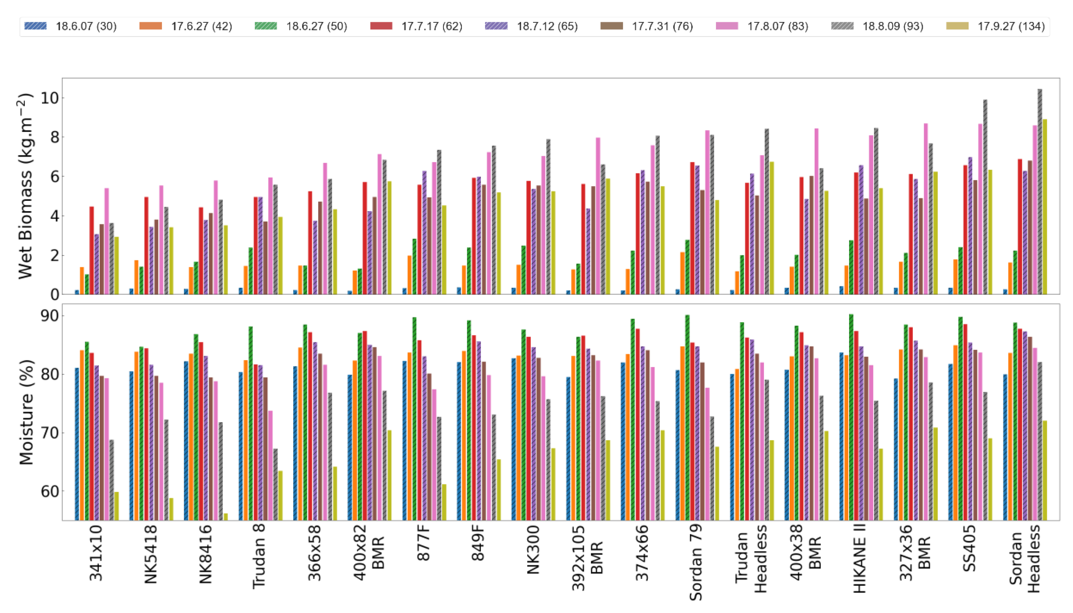
3.2. Ground Reference Data

Details of the experiment trials including sowing date, which differed by approximately one week, and harvest dates are provided in

Table 1. Experiment designs for the 2017 and 2018 growing seasons.

Trial	Year	Genotype	# of Plots	# of Genotypes	Sowing Date	Harvest Date	Available Biomass Data
HyCal-17	2017	Hybrid	72	18	16/05	27/09	27/06, 17/07, 31/07, 08/08, 27/09
InCal-17	2017	Inbred	120	60	16/05	27/09	27/09
SbBAP-17	2017	Inbred	760	350	16/05	28/09	28/09
SbDiv-17	2017	Inbred	1800	840	17/05	09/11	09/11
HyCal-18	2018	Hybrid	72	18	08/05	09/08	27/06, 12/07, 09/08
InCal-18	2018	Inbred	108	54	08/05	09/08	09/08
InCalTc-18	2018	Hybrid	108	54	08/05	06/08	06/08
SbDivTc-18	2018	Hybrid	1260	630	08/05	02/08	02/08 and 14/08
SNitTs-18	2018	Inbred	112	4	04/06	02/10	02/10

. For the HyCal-17 and HyCal-18 panels, biomass data were destructively collected multiple times during each growing season. For all other experiments, the biomass data were collected only once at the end of each growing season using a two-row combine harvester. The weight of the shredded plant material of each plot was considered as the fresh biomass value for that plot. After harvesting, around 500 g of the shredded plant material was used to determine the moisture content of each plot by measuring the fresh weight and dry weight (after drying the plant materials).

Figure 2 shows the distribution of the fresh biomass values for the experimental trials in the 2017 and 2018 growing seasons. Figure 2a,b shows the fresh biomass distribution of the HyCal-17 and HyCal-18 panels, respectively, during the growing seasons. In 2017, the biomass data on 27 June, 17 July, and 7 August were collected by hand harvesting one meter sections of three rows from each plot. Harvesting for all other dates was performed with a two-row combine harvester. These figures indicate that the genotypes have similar biomass early in the season but differ at the end of the season. Figure 2c shows the distribution of the end of the season biomass of the nine trials over both years: (1) the InCal-17 and SbDiv-17 are similar, (2) the HyCal-17 and HyCal-18 have similar shapes but different ranges of values, and (3) SbDivTc-18 and HyCal-17 are similar in both shape and range of values.

3.3. Remote Sensing Data

This study includes RGB, hyperspectral, and LiDAR remote sensing data collected by custom designed UAV platforms. All remote sensing data acquisition platforms were flown with global navigation satellite system/inertial navigation system (GNSS/INS) units for direct georeferencing. The description of the sensors used in this study is provided in

Table 2. Sensor Descriptions.

Sensor	Description
RGB	Sony Alpha ILCE-7R Sony 35mm Lens Full-frame 36.4MP
LiDAR	Velodyne VLP-16 600 rotations per minute (RPM), 360-degree horizontal FOV Maximum range of 100 m
VNIR	Headwall Photonics Nano-Hyperspec imaging sensor 272 spectral bands at 2.2 nm/band from 400 nm to 1000 nm 640 spatial channels at 7.4 µm/pixel, 12 mm lens (in 2017) and 8 mm lens (in 2018)
SWIR	Headwall Photonics Micro-Hyperspec pushbroom 166 spectral bands at 10 nm/band from 900 nm to 2500 nm 384 spatial channels at 24 µm/pixel, 25 mm lens

. RGB data for this study were collected using a Sony Alpha ILCE-7R RGB camera delivering high-resolution UAV-based aerial imagery. LiDAR data were collected with a Velodyne VLP-16 3D LiDAR sensor operating in the strongest return mode providing an average point cloud density of 750 points per m². Both the RGB camera and the VLP-16 sensor are mounted on a DJI Matrice 600 Pro (M600P) platform. Spatial and temporal system calibration for the datasets used in this study were conducted using the approaches described in [45] and [46], respectively. Additionally, the georeferenced orthomosaics were generated using the structure from motion strategies introduced in [47,48].

Visible near infrared (VNIR) and short wave infrared (SWIR) hyperspectral data were collected with two Headwall Photonics push-broom scanners. In 2017, the VNIR sensor was flown at an altitude of 60 m with a 12 mm Schneider lens, resulting in a ground sampling distance (GSD) of ~4 cm. An 8 mm lens was used in 2018, and the flying height was 40 m to maintain the GSD at ~4 cm and accommodate the field of view of other sensors on the platform. In both years, the SWIR sensor was flown with a 25 mm lens at 40 m, resulting in approximately a 4 cm GSD. In 2018, the VNIR and SWIR sensors were integrated and flown together on a single UAV platform. A rigorous boresight calibration process described by Habib et al. [49] was applied, yielding simultaneously collected co-aligned VNIR and SWIR data. Similar to [50], all the hyperspectral data were converted to reflectance using the empirical line method to relate the spectra collected from the UAV to data acquired by an SVC 1024i field spectrometer over the calibration targets placed in the field for each acquisition. The data acquired by the sensors in both 2017 and 2018 are listed in

Table A2. Remote Sensing Data Sets.

Year	Data Type	Field	Dates
2017	RGB and LiDAR	InCal, HyCal, SbDiv, and SbBAP	16/06, 21/06, 27/06, 05/07, 11/07, 14/07, 17/07, 25/07, 02/08, 08/08, 23/08, 3008
	VNIR	HyCal and InCal	21/06, 28/06, 04/07, 12/07, 18/07, 25/07, 08/08, 23/08, 30/08, 10/09, 15/09
		SbDiv	21/06, 27/06, 04/07, 18/07, 25/07, 30/07, 08/08, 14/08, 23/08, 10/09, 24/09, 30/09
		SbBAP	21/06, 27/06, 04/07, 18/07, 25/07, 30/07, 08/08, 14/08, 23/08, 10/09, 24/09
	SWIR	InCal and HyCal	23/08, 30/08, 10/09, 15/09
		SbDiv	02/08, 08/08, 14/08, 23/08, 30/08, 10/09, 30/09
		SbBAP	02/08, 08/08, 14/08, 23/08, 30/08, 10/09
2018	RGB and LiDAR	HyCal, InCal, InCalTc, and SbDivTc	22/05, 29/05, 04/05, 11/06, 20/06, 27/06, 02/07, 11/07, 18/07, 23/07, 01/08, 06/08
		SNitTs	28/06, 03/07, 11/07, 17/17, 23/07, 01/08, 06/08, 16/08, 25/08, 05/09, 19/09
	VNIR and SWIR	HyCal, InCal, InCalTc	04/06, 08/06, 14/06, 29/06, 03/07, 06/07, 11/07, 18/07, 25/07, 02/08, 09/08
		SbDivTc	04/06, 08/06, 14/06, 29/06, 03/07, 06/07, 10/07, 11/07, 25/07, 02/08
		SNitTs	28/06, 03/07, 11/07, 18/07, 25/07, 02/08, 13/08, 28/08, 04/09, 12/09, 18/09

in Appendix A.

3.4. Feature Extraction

As discussed earlier, it is important to extract features that are related to the specific trait of interest and are preferably not redundant. In this study, both traditional and new candidate features focused on the relevance to biomass prediction were extracted from rows 2 and 3 of the 4- or 12-row plots to minimize the border effect. For each acquired data set (listed in Table A2 in Appendix A), we extracted the features described in the following sections.

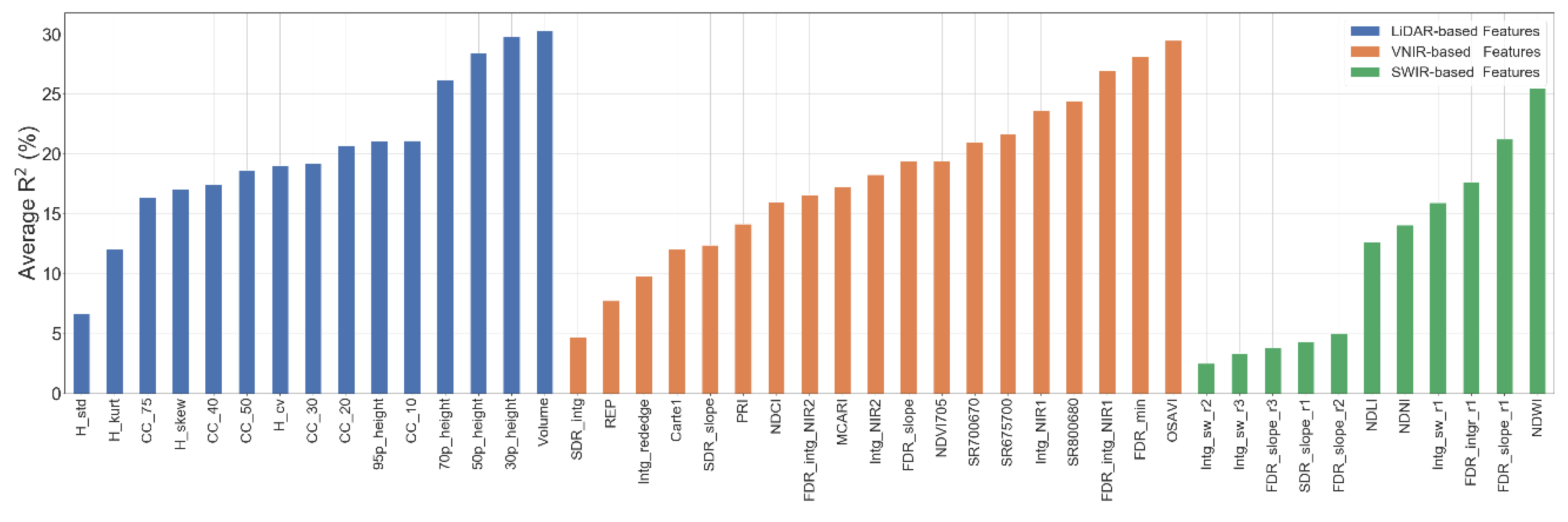
3.4.1. Hyperspectral-Based Features

• Spectral Reflectance

From the Hyperspectral Imaging (HSI) data, the average reflectance values of the plots were calculated from rows 2 and 3 of each plot after masking the shadow and soil pixels.

• Vegetation Indices

Vegetation Indices (VIs) obtained from HSI data have been widely used in different applications, as they are computationally simple and representative of the relevant chemically interpretable absorption and reflectance features in the spectrum. In this study, 13 vegetation indices, listed in

Table A3. Vegetation indices extracted from each HSI spectrum.

Data Type	Index Name	Formulation	References
VNIR	NDVI	(R750 − R705)/(R750 + R705)	[70]
	NDCI	(R762 − R527)/(R762 + R527)	[71]
	Carte1	R695/R420	[72]
	SR800,680	R800/R680	[73]
	SR675,700	R675/R700	[74]
	SR700,670	R700/R670	[75]
	OSAVI	(1 + 0.16) (R800 − R670)/(R800 + R670 + 0.16)	[76]
	MCARI	[(R700 − R670) − 0.2(R700-R550)](R700/R670)	[77]
	REP	700 + 40[(R670 + R780)/2 − R700)]/(R740 − R700))	[78]
	PRI	(R531 − R570)/(R531 + R570)	[79]
SWIR	NDWI	(R860 − R1240)/(R860 + R1240)	[80]
	NDLI	[log(1/R1754) − log(1/R1680)]/[log(1/R1754) + log(1/R1680)]	[81]
	NDNI	[log(1/R1510) − log(1/R1680)]/[log(1/R1510) + log(1/R1680)]	[81]

in Appendix A were extracted and used in the predictive models.

• Integration Features

NIR bands are particularly important for representing plant physiology but are subject to the time during the growing season and environmental conditions. The area under the spectral curve for a given range from λ_a to λ_b is defined as $Intg\left({\lambda }_a,{\lambda }_b\right)={{\displaystyle \int }}_{{\lambda }_a}^{{\lambda }_b}S\left(\lambda \right)d\lambda$, where $S\left(\lambda \right)$ is the reflectance at $\lambda$ nm. Using different ranges of spectral values, six features were extracted from each HSI spectrum as listed in

Table A4. Integration features extracted from each HSI spectrum.

Data Type	Feature Name	λa	λb
VNIR	Intg_rededge	685	745
	Intg_NIR1	770	910
	Intg_NIR2	910	1000
SWIR	Intg_SWIR_r1	920	1353
	Intg_SWIR_r2	1430	1800
	Intg_SWIR_r3	1952	2385

in Appendix A.

• Derivative Features

The spectral derivatives, which quantify slope, curvature, and higher-order aspects of reflectance spectra, can be useful by revealing spectral features that may not be apparent in reflectance data alone [51]. For example, the “red-edge” position (between 680 nm and 750 nm) in crop reflectance data can be easily identified in the derivative spectra, and has been related to crop biomass [52]. Feng et al. analyzed 20 spectral derivative features near the red edge area to estimate wheat leaf nitrogen concentration [53]. In this study, the polished spectra were calculated using a Savitzky–Golay filter [54], then the first derivative (FDR) and second derivative (SDR) of the spectra were extracted. From FDR and SDR, 11 features were extracted and used in the additional analysis as described in

Table A5. Derivative features were extracted from each first derivative (FDR) and second derivative (SDR) spectrum.

Data Type	Feature Name	Description
VNIR	FDR_slope	slope of the line that passes through the minimum of FDR and the maximum of FDR in 660–690 nm range
	FDR_min	minimum of FDR
	FDR_intg_ NIR1	integration of FDR in bands between 670 and 780 nm
	FDR_intg_ NIR2	integration of FDR in bands between 910 and 1000 nm
	SDR_slope_rededge	slope of the line passing through the maximum and the minimum of SDR
	SDR_intg	integration of SDR in all bands
SWIR	FDR_slope_r1	slope of the line that passes through the maximum of FDR in 1000–1050 nm range and the minimum of FDR in 1100–1200 nm range
	FDR_slope_r2	slope of the line that passes through the maximum of FDR in 1475–1525 nm range and the minimum of FDR in 1675–1725 nm range
	FDR_slope_r3	slope of the line that passes through the maximum of FDR in 2000–2050 nm range and the minimum of FDR in 2200–2300 nm range
	FDR_intg-r1	integration of FDR in bands between 920 and 1353 nm
	SDR_ slope_r1	slope of the line that passes through the maximum of SDR in 1100–1200 nm range and the minimum of SDR in 1000–1100 nm range

in Appendix A. These features were selected at wavelengths where spectra of the varieties differed and were also uncorrelated.

3.4.2. LiDAR-Based Features

The 3D structural characteristics of the plants in a plot can be described using various features extracted from LiDAR data. The digital terrain model (DTM) was derived from LiDAR data acquired before the emergence of the plants in each field by interpolating the LiDAR point cloud into a regular grid (8 × 8 cm in this study) using the nearest neighbour interpolation method. The DTM represents the bare earth height information and is assumed to be constant throughout the growing season. For each point cloud data acquired throughout the season, the height of points in the was estimated by subtracting the DTM from the “z” coordinate of each point. Then, the following features were extracted from the point cloud of each plot:

• Height Percentile

To capture the vertical distribution of the LiDAR points in each plot, the 30th, 50th, 75th, 90th, and 95th percentile height values from the point cloud of each plot were calculated.

• Canopy Volume

To estimate volume related characteristics of the canopy in each plot, a grid with cells of size 8 × 8 cm was assigned to each plot, and then the associated height was calculated from the points located in each cell, multiplied by the size of the cell to estimate the volume of the canopy within each cell. The aggregate “volume” in each plot is referred to as the volume of the vegetation within a plot. The height of each cell in this study was calculated as the average of the height of the lowest point and the height of the highest point in each cell.

• Canopy Cover

Canopy cover can be estimated from LiDAR data as the ratio of above-ground points (or, canopy points) to the total number of LiDAR points in a given area. The following approach was used in this study for canopy cover estimation for each plot. First, the field is divided into grid cells of a user-defined dimensions (8 × 8 cm in this study, consistent with the canopy volume calculation). Then, for each grid cell, the LiDAR points are split into two groups, canopy points and bare earth based on their height using a user-defined threshold. The points above the threshold are considered as canopy points. The canopy cover is estimated as the ratio of the number of canopy points to the total number of LiDAR points in each cell. The average of the canopy cover estimated for the cells located in each plot is assigned as the canopy cover for that plot. In this study, candidate threshold values were 0.1, 0.2, 0.3, 0.4, 0.5, and 0.75 multiplied by the 95th percentile height of each plot, resulting in six height-dependent canopy cover related features.

• Height Statistics

The spatial distribution of the height of the LiDAR points in each plot can also be represented using statistical moments of the distribution. These statistics can also be included as candidate input features for predictive models.

3.5. Regression-Based Modeling Approaches

Common regression-based approaches such as partial least squares regression (PLSR), support vector regression (SVR), and random forests (RF) are widely utilized to build predictive models with remote sensing based inputs. PLSR reduces a potentially large number of measured collinear input variables to a few uncorrelated latent variables while seeking to explain the maximum multi-dimensional variance of the dependent variable via a linear model. PLSR has been investigated for developing predictive models to estimate leaf biochemical and biophysical properties [55], chlorophyll content [56], carotenoid content [57], relative water content [58], protein, lignin, and cellulose [59], leaf nitrogen content [60], LAI [61], and biomass [34].

SVR is a supervised non-parametric regression technique, and therefore, no assumptions regarding the underlying data model are required. The original feature space is transformed into a higher dimensional space [62], with the goal of finding a hyperplane to predict the training data set. The optimal values of the kernel function parameters were obtained in this study by a general k-fold cross-validation in a grid search.

Random Forest (RF) modeling is an ensemble learning technique which uses a large set of classification and regression trees (CART) to predict the variable of interest [63]. In random forest regression, each tree is built by randomly choosing a set of variables and a subset of training samples with replacement. The selected samples are used for training, and the remaining observations are used in an internal cross-validation process to determine the performance of the RF model. The outputs of all trees are aggregated to produce a final prediction. A review of RF modeling in remote sensing applications is available in [64]. Similar to SVR, the parameter optimization was accomplished by a general k-fold cross-validation in a grid search method. A grid search method was used to select the best hyperparameters for each model.

Table A6. Grid search parameters for regression methods.

Algorithm	Hyperparameter	Values Tested
PLSR	Number of components	2, 3, 5, 10, 15, 20
SVR (RBF)	C	10, 100, 1000, number of features
	gamma	1/n, 0.0001, 0.001, 0.01, 0.1
Random Forest (RF)	Max tree depth	5, 10, 100
	Min sample split	2, 10
	Number of trees	50, 100, 500

lists the candidate parameters that were tested for each method in the grid search process. The Anaconda Distribution of Python version 3.7 with the Scikit-learn library [65] was used for conducting grid search and developing regression models.

3.6. Statistical Analysis

The one-way analysis of variance (ANOVA) is used to determine whether there is a significant difference among the groups of data. If there is a significant difference, then an honest significant difference (HSD) Tukey test (with α = 0.05) can be conducted to determine which groups are significantly different from each other. We also use two-way ANOVA, to evaluate combinations of several variables or factors to identify those that have a significant effect on the estimates [66]. Prior to these statistical tests, the normality and homoscedasticity were confirmed by visually inspecting the variables. The statsmodels library [67] was used for data preparation and statistical analysis.

4. Results

4.1. Data Screening

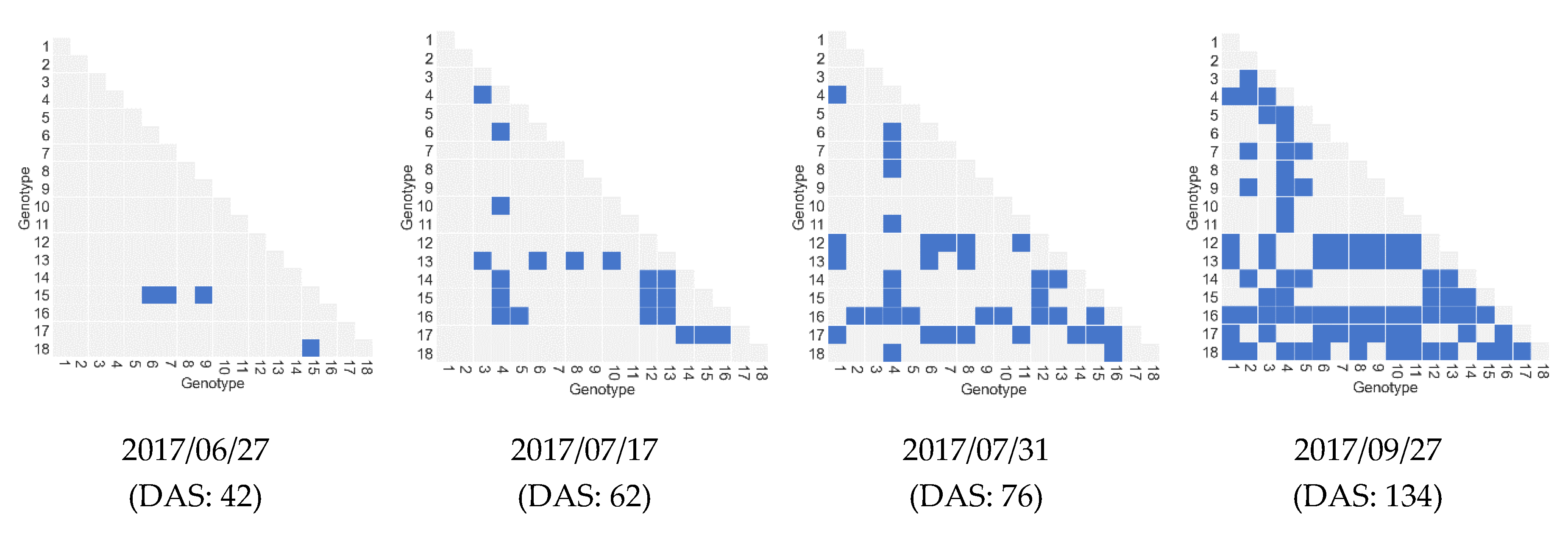
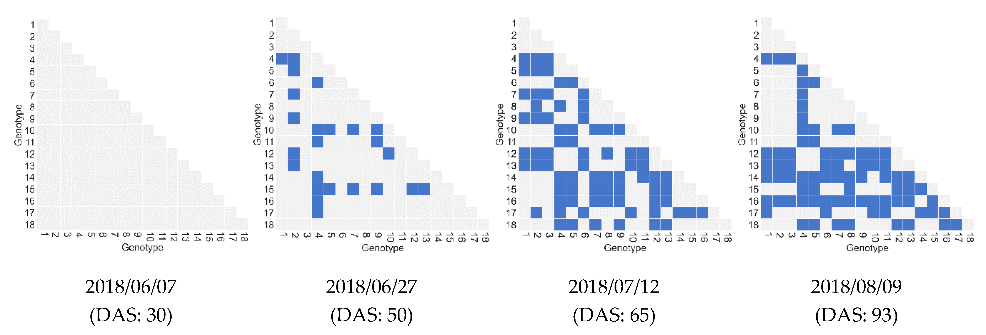
4.1.1. Time Series of Biomass Data

In the 2017 and 2018 growing seasons, the destructive biomass data were collected multiple times (approximately every month) from the hybrid calibration panels. Figure 3 shows the fresh weight and moisture content of the 18 sorghum varieties planted in the HyCal-17 and HyCal-18 experiments. The moisture content increases at the beginning of the season until it reaches its maximum at 50 to 60 days after sowing. The fresh weight of the plants also increases rapidly at the beginning of the season, while at the end of the season, it decreases as the plants senesce. Among the varieties shown in Figure 3, those that are photoperiod sensitive (“Sordan Headless” and “Trudan Headless”) did not flower in the environment in which these experiments were conducted, and continued to add plant material until the end of the season.

Each variety has four replicates in the hybrid Calibration panels, providing adequate sample data to compare the relationship across the varieties and associated changes during the growing season. For each date that the biomass data were collected, an ANOVA test was conducted on the fresh biomass, and if it indicated variability among the varieties was highly significant, a Tukey’s multi-comparison test was performed. Figure 4 shows the results of Tukey’s pairwise multi-comparison test (α = 0.05) for the fresh biomass data collected in the 2017 and 2018 growing seasons. In general, at the beginning of each season, only a few varieties were significantly different, while the variability among the varieties at the end of each growing season was greater. From Figure 4 it is also clear that the two photoperiod sensitive varieties (varieties 16 and 18) were significantly different from the other varieties at the end of both 2017 and 2018 growing seasons.

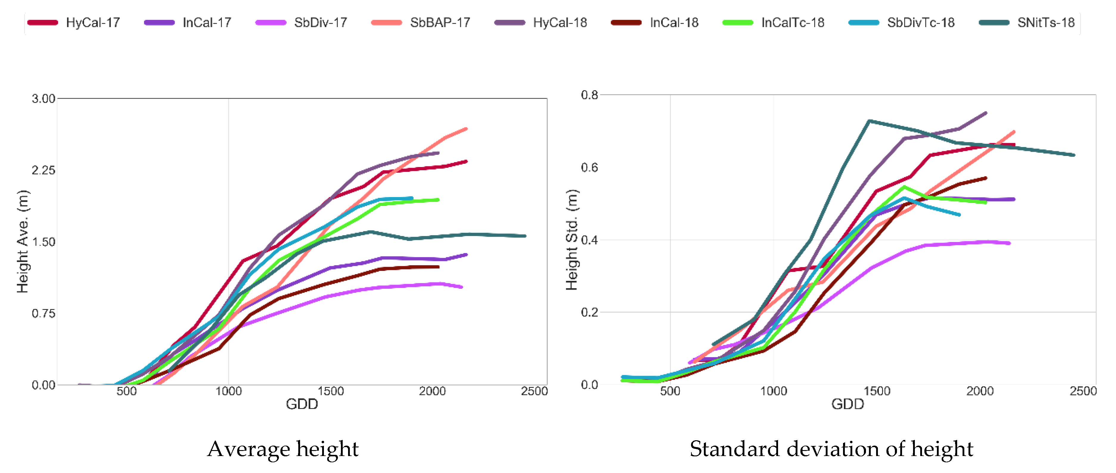
4.1.2. Time Series of Remote Sensing Data

RS spectral signatures varied both across phenotypes and during the growing season. Figure 5 shows the average spectra of the 18 varieties of sorghum in the HyCal-18 panel on 18 July 2018 (day after sowing (DAS) = 71) (see Figure A4 in Appendix B for the variance plot). On that day, the signatures of the 18 varieties were very similar in the visible range of the spectrum, but there was more variability in the NIR portion of spectrum that may reflect variation in biochemical features, including lignin type and composition associated with the brown-midrib (bmr) traits. Figure 6 shows the reflectance of one of the varieties from June to September which shows there is very little change in the visible range of the spectrum, and especially in the blue and green bands, while the reflectance in NIR bands changes from about 35% to 60% on average (see Figure A5 in Appendix B for the variance plot). The maximum reflectance values were observed in the range of 750–850 nm on 3 July (DAS = 56). One of the reasons for changes in the reflectance for sorghum is the appearance of the panicles, which emerge a few days before the flowering date (the date on which 50% of panicles in a plot are flowered). Field notes indicate that the flowering date for “Trudan 8” was 10 July 2018.

Figure 7 shows the Digital Surface Model (DSM) generated from the LiDAR point cloud for the SbDivTc-18 panel from multiple dates in the 2018 growing season. From Figure 7, the plots are more similar at the beginning of the season, with greater differences later in the season. Figure 8 shows the point cloud data for two plots (rows 2 and 3) of the HyCal-18 experiment for multiple dates in the 2018 growing season. “341 × 10” is a dwarf grain sorghum variety (Figure 3), while “Trudan Headless” is a photoperiod sensitive forage sorghum with high biomass accumulation.

Figure 9 shows the mean and standard deviation of the height of all the plots for all the experiments in the 2017 and 2018 growing seasons extracted from the LiDAR point clouds, providing structural characteristics of the varieties planted in each experiment. For both HyCal-17 and HyCal-18, the height increases as the headless varieties continue to grow until the end of the season. The SbBAP-17 experiment also has the maximum average height at the end of the season, as it includes many plots of photoperiod sensitive genotypes that do not flower. The InCal-17, InCal-18, and SbDiv-17 include similar inbred varieties; thus, they have a very similar average height (also the lowest height values among the experiments). As was noted earlier, a histogram of the height of the points from the LiDAR point cloud provides information about the distribution of different height values in a plot. This genotype dependent information may be discriminating in predictive models. Figure A3 in Appendix B shows the histograms for the dwarf grain sorghum 341 × 10 and the photoperiod sensitive Trudan Headless varieties in the HyCal-17 experiment.

The multi-temporal and cross-correlations during the growing season can be useful for screening for redundant features. Figure 10 shows the correlation matrices for the OSAVI and LiDAR-based canopy cover calculated using the combined data acquired over the HyCal-17 experiment in the 2017 growing season. It illustrates the rapid changes at the beginning of the season, especially prior to the flowering time (second week of July for this experiment) which is associated with the rapid growth of the plants. From Figure 10, OSAVI changed more than the canopy cover during the early season, and end of season OSAVI values have lower inter-temporal correlation compared to the correlation between the canopy cover values on corresponding dates.

Similar to the last section, Figure 11 and Figure 12 show the results of the multiple-comparison Tukey’s test for the OSAVI and volume features for the HyCal-17 and HyCal-18 experiments on multiple dates during the 2017 and 2018 growing seasons. These results are consistent with the results of Tukey’s test conducted on biomass data in the previous section, which greater variability among the varieties at the end of each growing season.

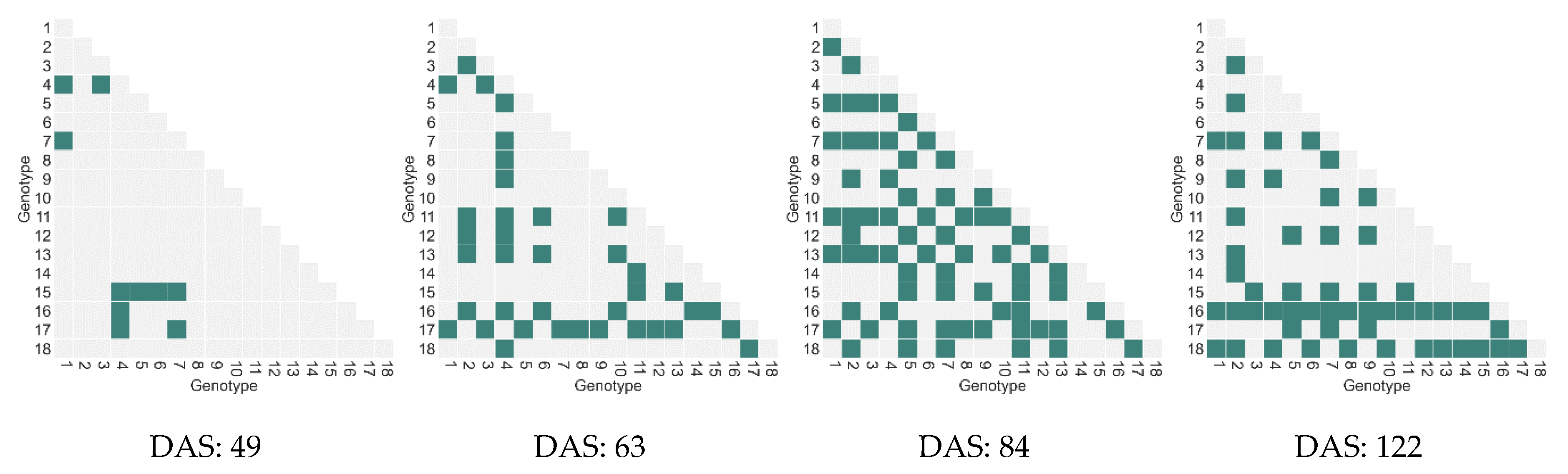
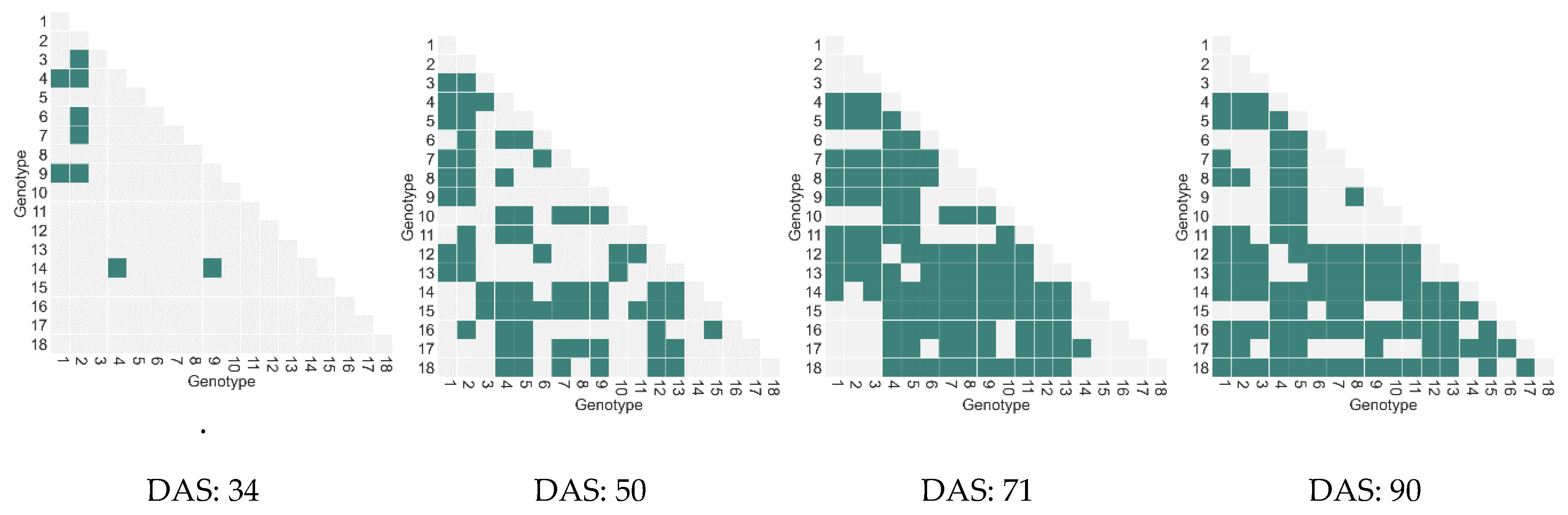
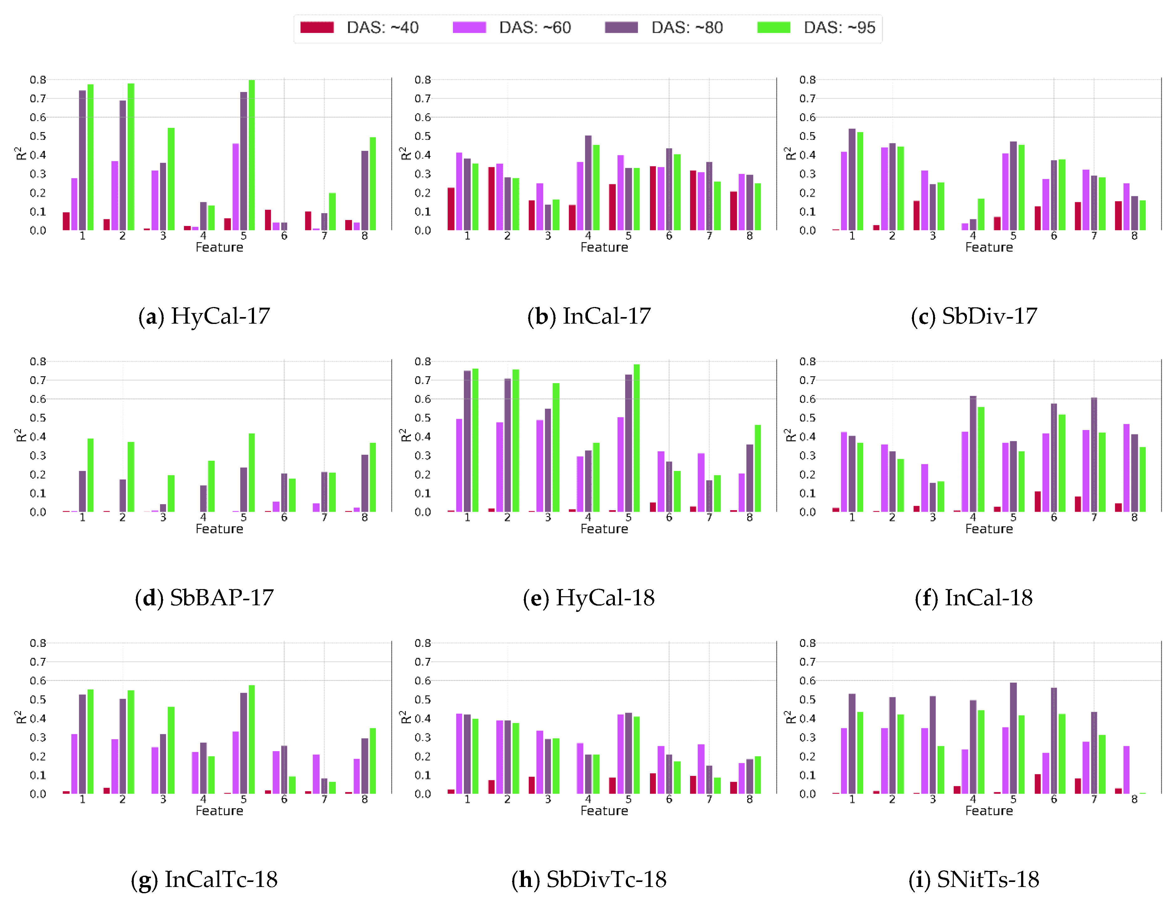
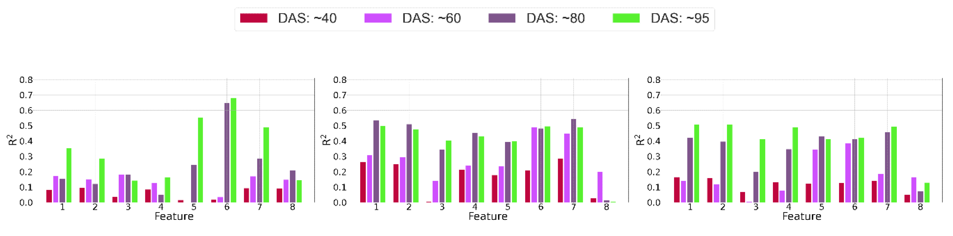
4.1.3. Relationship between Features and Biomass

In this section, the relationship between the biomass data and RS features, as well as the change in their relationship during the growing season, is discussed. Figure 13 shows one feature from LiDAR (90th percentile height of the plants), one feature from hyperspectral data (Intg_NIR1), and the biomass data for the dwarf grain sorghum 341 × 10 and the photoperiod sensitive Trudan Headless varieties, both from the HyCal-17 and HyCal-18 experiments (one with low and one with high biomass values). To compare the data from the two years at the same stage of growth, the data are plotted versus growing degree day (GDD), a heat index calculated from temperature data for each day [68]. At GDD of 2100, the biomass in 2018 for both varieties was slightly higher than in 2017 (as noted in Table 1, the HyCal-18 was planted two weeks earlier than HyCal-17). The height data, Intg_NIR1, and biomass data follow the same pattern of change over time for each variety in both growing seasons. The height for the photoperiod sensitive variety (“Sordan Headless”) always increases, while other varieties stop growing around flowering time (GDD of 1500); the Intg_NIR1 increases rapidly earlier in the season, and then gradually decreases at around GDD of 1500 until the end of the season; the biomass continues to increase, and especially for the photoperiod sensitive variety. Inter-annual differences also inherently include the impact of the timing and quantity of rainfall.

For each feature extracted from the RS data, the simple prediction potential (R²) and associated changes during a season were investigated using linear regression-based models for the end of season biomass prediction. Robust features should be applicable across the varieties, at least for common experiments. Figure 14 and Figure 15 show the R² values of the models for each feature extracted from LiDAR and hyperspectral VNIR data, at four stages of growth and for all nine experiments conducted in the 2017 and 2018 growing seasons. From Figure 14, the 30th percentile height and volume features provided the highest R² values for predicting the end of season biomass among the LiDAR-based features for both HyCal-17 and HyCal-18 experiments, as the varieties in those experiments were more diverse in their structural characteristics, providing strong potential for biomass prediction using geometric-related features. The R² values for different LiDAR-based features in the InCal-17, InCal-18, and SbDiv-17 experiments are very similar, which is consistent with Figure 9; they all have the lowest average height and lowest variability in height compared to the other experiments, resulting in lower R² values for these experiments compared to the experiments with hybrid cultivars. For both InCal-17 and InCal-18 experiments, the highest R² values were obtained from feature #5 (coefficient of variation of height), which is representative of the distribution of the points in the canopy point cloud. The R² values of the models developed for the SbDivTc-18 and InCalTc-18 are lower than the HyCal-17 and HyCal-18 experiments, but the same features (features #1, #2, and #5) provided the maximum R² for all of these experiments, which include hybrid cultivars. The SbBAP-17 also includes hybrid cultivars; however, the R² values for all the features are lower compared to all other experiments, mainly because the last LiDAR data were collected on August 30th, and included many photoperiod sensitive cultivars which grew until the final biomass data were collected at the harvest (28 September). Other varieties did not grow during this time, which impacted the biomass–height relationships. Generally, for the experiments with the hybrid cultivars (refer to Table 1), the late season data sets provided the highest R², while for the experiments that included inbred cultivars, the data sets of GDDs yielded the lowest R² values.

For the hyperspectral features shown in Figure 15, the highest R² values are associated with InCal-17 and InCal-18, collected on ~80 DAS, while for other experiments, the dataset of ~95 DAS yielded the highest R² values. Moreover, the same pattern for R² values for the features of the InCal-17, InCal-18, and SbDiv-17 was observed. For these panels, the R² is generally higher than the panels that include hybrid cultivars.

Given similar trends of the regression models shown in Figure 14 and Figure 15, the models were developed across all the experiments for each of the features, and all the available dates to investigate the potential for using a common set of features for all experiments and times for the multiple input predictive models. The average R² for each feature, from all the dates and all the experiments is provided in Figure 16, which shows volume, 30th percentile height, OSAVI, FDR-min, and NDWI features had the highest average R² from LiDAR, VNIR, and SWIR data sets, respectively. Linear regression models were also developed for the individual band values from both hyperspectral VNIR and SWIR data. The average and maximum R² for each band from all the dates and all the experiments are shown in Figure 17, which shows that the area of spectrum between 750 and 1100 nm provided the highest R² for the linear regression models. While the R² values for some experiments and some dates for the bands in 2000–2300 nm are relatively high (30–60%), the average R² values are much lower in comparison to the 750–1100 nm range.

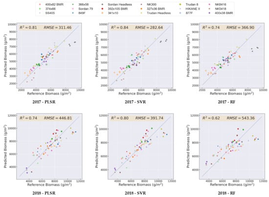
4.2. Biomass Predictive Models

In this section, the results related to the impact of different regression methods, the time of biomass sampling and remote sensing data acquisition, and the number of samples on the prediction results are provided.

4.2.1. Impact of the Data Source and Regression Method on the Prediction Results

To evaluate the performance of different regression-based modeling approaches, PLSR, SVR, and RF were implemented for end of season biomass prediction using the LiDAR and hyperspectral data collected in each growing season. Figure 18 shows the R² values of the predictions relative to the reference data for all the experiments, using six data sources (LiDAR, VNIR, SWIR, and combinations), and the three methods. For each prediction with a data source, all available data sets over the whole season were used for training and validation of the models, where two thirds of the sample data (or a maximum of 200 samples) were randomly selected 100 times for the training of the algorithm, and the remaining samples were used for cross validation via the hold-out method. For all the experiments except the SNitTs-18, all the replicates of a variety were assigned to either the training or test sets to avoid any impact from the number of replicates on the prediction results. SNitTs-18, however, included only four varieties, and a different number of replicates for each variety; thus, the training and test sets were assigned randomly from the plots regardless of their varieties for this experiment. Potential reasons for differences in predictions include:

(i)

Diversity in the samples: the regression models are better able to learn the pattern in the data when the samples are more diverse.

(ii)

Number of data samples: the larger the number of data points in an experiment, the higher accuracies are typically achieved for the prediction.

(iii)

Similarity between the training and test data sets; if the training and test data sets are very different, then overfitting can occur for the training data set, resulting in decreased accuracy of the predictions. Note that this can happen when the number of data samples is limited, which causes unlike training and test sets, even when the samples are selected randomly. Additionally, if there is a significant range of biomass values in one experiment, there is more chance to have dissimilar training and test sets.

Figure 18 shows that the highest accuracy of end of season biomass prediction using all combinations of data sources was achieved for the SNitTs-18 experiment. There were two nitrogen treatments in this experiment; half of the plots in this experiment were fertilized with 250 kg/ha nitrogen while the other half were not fertilized, causing high and low biomass values for the plots, high diversity in the reflectance data from the hyperspectral images, as well as high diversity in geometric-based features extracted from LiDAR point cloud (reason i). As was noted, samples were assigned to the training and test sets for this experiment differently from the other experiments, causing multiple samples of each variety to be assigned to both the training and test sets, resulting in increased similarity in the two sets (reason iii).

The highest accuracy of prediction using LiDAR features as the sole input was obtained for the HyCal-17 and HyCal-18 experiments, which include hybrid cultivars that are more diverse in structural characteristics compared to the inbred cultivars; thus, the regression model can distinguish and relate the LiDAR-based features to the biomass data (reason i), which is consistent with the results in Figure 14. In general, the predictions are more accurate for the experiments that include hybrid cultivars. As was shown in Figure 9, the InCal-17, InCal-18, and SbDiv-17 have the smallest standard deviation in the LiDAR-based height, indicating that the associated varieties have similar structural characteristics.

The predictions for the SbDiv-17 are more accurate than the predictions for the InCal-17 as more samples were available for the training set, 200 for SbDiv-17, and 80 for InCal-17 (reason ii). For the SbBAP-17, the prediction accuracies are lower than most of the other experiments. This experiment included varieties that were highly diverse in terms of structural characteristics (Figure 9), also had a much larger range compared to the other experiments. This resulted in dissimilar samples in the training and test sets (reason iii). Figure 19 shows a box plot for the fresh biomass data for all the experiments, and the SbBAP-17 experiment had the greatest range of biomass values among the experiments, the lowest accuracies for the predictions, while SNitTs-18 experiment has the smallest range and the highest R² values for the predictions.

For HyCal-17 and HyCal-18 experiments, PLSR, SVR, and RF models were developed using all three data sources and leave-one-out cross validation strategy, where in each fold, one variety was assigned as test and the other 17 varieties were included in the training set. The results are shown in Figure 20. For both experiments, the SVR method provided the highest R² values for the predictions. For HyCal-17, all three regression methods underestimated the value of the biomass for one of the photoperiod varieties (which also had the maximum biomass, as noted previously); however, the RF model had the lowest accuracy. RF for both years resulted the lowest R² as a result of overfitting as was discussed earlier. All three methods resulted in predictions with lower accuracies for the experiment in 2018 compared to 2017, which could be because the end of season biomass data were measured at an earlier date in 2018, when all the plants had not reached full maturity.

4.2.2. Predictions in Time

To evaluate the capability of remotely sensed data for predicting biomass through the growing season, SVR models were developed for six dates in the 2017 and 2018 growing season for the HyCal-17 and HyCal-18 experiments. The R² values of the predictions relative to the reference data are shown in Figure 21. For each prediction, all the VNIR hyperspectral and LiDAR data collected prior to the date of biomass measurement were used in the SVR models. The R² values of the predictions at the beginning of the season were lower compared to the end of the season, especially when using only VNIR features. Early season growth is focused on the production of biomass from stalks and leaves, while mid-season development is related to flowering and early development of panicles. Plant structural characteristics do not change significantly after flowering in the mid-season, while spectral characteristics change significantly especially during flowering with the emergence of the panicles.

4.2.3. Multi-Temporal Predictions of End-of-Season Biomass

It is highly desirable to predict the end-of-season biomass as early as possible during the growing season to avoid unnecessary investment of phenotyping resources in non-productive varieties. The SbBAP-17, SbDiv-17, and SbDiv-18 were chosen to conduct the evaluations in this section as they had an adequate number of samples as well as RS data points and included both hybrid and inbred cultivars. Figure 22 shows the accuracy of end-of-season biomass predictions for these experiments using hyperspectral VNIR, SWIR, and LiDAR data from each date individually, and in combination with the earlier dates. For both SbBAP-17 and SbDiv-17 experiments, the earliest data set yielded very low prediction accuracies. For SbBAP-17, the best results when using features from individual sensors for VNIR and SWIR data sets were achieved from 10 September with R² = 0.60 and R² = 0.54, respectively. Based on LiDAR data, 23 August resulted in the highest values, with R² = 0.46. For the SbDiv-17 experiment, the combined VNIR and LiDAR data sets of 25 July and 2 August provided the highest accuracy of using individual data sets. For SbDivTc-18, the data inputs from 11 July resulted an R² of 0.75, which indicates the July data sets have good potential for biomass predictions. For all three experiments, the best results were obtained when features from all the hyperspectral and LiDAR data sets from the whole season were used, resulting in R² of 0.63, 0.75, and 0.78 for the SbBAP-17, SbDiv-17, and SbDiv-18 experiments, respectively. Although the best results were obtained using the whole season RS data, the models developed using middle season data (DAS of ~60 to 80) were also able to provide comparable accuracies.

4.2.4. Impact of the Number of Features and Samples on Biomass Prediction

As noted earlier, measuring biomass in the field is time-consuming and expensive; however, it is still required for training the regression models. Generally, the greater the number of samples for training, the more accurate the predictions. To evaluate the impact of the number of samples in training set, the SVR and PLSR models are developed for end-of-season biomass prediction using all the data sources and various numbers of samples in the training set. Each model was trained with a specific number of samples, and the process was repeated 100 times, each time with a different, but same sized set of randomly selected samples. The rest of the available samples were assigned to the testing set. Figure 23 shows the median and standard deviation of the R² values of developed models for some of the experimental trials. The R² of predictions for both SVR and PLSR models increase as the number of training samples increases. However, the accuracy of PLSR models is higher than SVR models when a smaller number of training samples is used. The rate of increase of R² with the respective increases in the number of training samples is higher for SVR compared to PLSR; thus, when the maximum of available samples is used in training for experiments (e.g., for SbDivTc-18), the SVR models had higher R² values. For all the experiments, the standard deviation of the R² values decreases as the number of training samples increases, showing more reliable (repeatable) prediction models are developed when more samples are available for training, as expected. However, for some experiments such as HyCal-17, the standard deviation of R² decreases initially, reaches a minimum, then increases. This is attributed to the small total number of samples: using more samples in the training set implies a smaller number of samples is available in the test set.

5. Discussion

The predictions results with respect to the diversity, number of samples, and similarity between test and training sets for all the experiments are summarized in

Table 3. Summary of the prediction results of the experimental trials.

	HyCal-17 and 18	InCal-17 and 18	SbBAP-17	SbDiv-17	InCalTc-18	SbDivTc-18	SNitTs
Diversity	Very High	Low	Very High	Low	High	High	High
Number of samples	Low	Low	High	High	Low	High	Low
Test-training set dissimilarity (range of biomass)	High	Low	Very High	Low	High	High	Low
Prediction accuracy (maximum R2)	High (0.80)	Medium (0.71)	Medium (0.67)	Medium (0.74)	Medium (0.69)	High (0.77)	Very high (0.88)

.

In general, for the experiments with hybrid cultivars, RF models had lowest prediction accuracies among the three methods, which is related to the fact that there was more dissimilarity between the training and test sets in both RS and biomass data among the hybrid cultivars compared to those that were inbred, and RF models can be overfitted to the training data set; thus, they may not provide as accurate predictions as SVR and PLSR. For the InCal-18, however, RF yielded the highest accuracies for most of the data sources. For the experiments with a sample size of 200 (SbDiv-17, SbBAP-17, and SbDivTc-18), the SVR models provided the most accurate results, while for the experiments with a lower number of data samples, PLSR provided the highest prediction accuracies.

A summary of the prediction results for various data sources and regression methods is provided in Figure 24, where the R² values of the nine experiments are shown in a box plot (RMSE values are shown in Figure A6 in Appendix B). For the LiDAR data, the RF method provided slightly higher median accuracies than PLSR and SVR, with lower variability in R² values (more reliability). When VNIR data was the only input, PLSR yielded more accurate results, which is similar to the results obtained in [10] yield prediction of potatoes using VNIR hyperspectral data. For all other data sources, SVR yielded a higher median R². For SWIR and VNIR combined with SWIR sources, SVR provided more reliable results, while for VNIR, VNIR combined with LiDAR, as well as a combination of all data sources, PLSR provided more reliable results. Also, the SVR models provided the maximum R² for all the data sources.

Similar to the study by Almeida et al. [69], an ANOVA test was performed on the prediction results to determine the impact of the method and data source (e.g., sensor-based features) on the prediction results. The ANOVA results provided in

Table 4. Analysis of variance of the R² respective to the data source, regression method, and their interaction.

Factor	Sum of Squares	Degree of Freedom	F Value	p-Value	ɳ2 (%)
Data source	103.70	5	564.09	<2 × 10−14	68.59
Method	17.15	2	233.23	<2 × 10−14	28.36
Data source:method	9.24	10	25.14	<2 × 10−14	3.06
Residuals	594.95	16,182

show that the data source is the cause of 69% of the variation in the prediction results, 28% for the regression method, and 3% for the interaction their interaction. These results are consistent with those of [33,69]. This indicates that the data source should also be considered to determine the regression method in the design of similar experiments. A similar ANOVA test was performed on the R² values for six experiments, including HyCal-17, HyCal-18, InCal-17, InCal-18, SbDiv-17, and SbDiv-18, of which three include hybrid cultivars, and three include inbred cultivars. On this test, the cultivar type (hybrid or inbred) was considered as the third factor. Recall that the sorghum hybrid cultivars are more variable in their characteristics than inbreds in terms of biomass and structural characteristics. The results of this test in

Table 5. Analysis of variance of the R² respective to the data source, regression method, cultivar type, and their interactions.

Factor	Sum of Squares	Degree of Freedom	F Value	p-Value	ɳ2 (%)
Data source	80.95	5	412.58	<2 × 10−6	44.18
Method	19.29	2	245.79	<2 × 10−6	26.32
Cultivar type	0.35	1	8.86	0.003	0.95
Data source:method	6.84	10	17.44	<2 × 10−6	1.87
Data source:cultivar type	4.03	5	20.53	<2 × 10−6	2.20
Method:cultivar type	17.59	2	224.12	<2 × 10−6	24.00
Data source:method:cultivar type	1.82	10	4.63	0.093	0.50
Residuals	422.37	10,764

indicate that the data source also has the highest contribution to the variation in the predictions (44%). The regression method is the cause of 26% of the variation in the prediction results, and less than 1% is attributed to the cultivar type. However, the interaction between the regression method and cultivar is responsible for 24% of the variation, suggesting that the cultivar type is another important factor to consider when determining the regression method for developing predictive models.

Recommendations for Biomass Prediction

In this section, we summarize the findings of the tests conducted in this paper in the format of recommendations to achieve reliable biomass prediction. The recommendations are based on the data, the genotypes, and the location where the study was conducted; thus, they might not be generalizable.

• Regression Model

Both PLSR and SVR models provided more accurate predictions than RF. SVR generally provided more accurate predictions, however, PLSR is preferable when the number of sample data points is very limited (less than 50 samples) as well as when high variability in the biomass data is expected.

• Data Source

ANOVA analysis on the prediction results showed that the data source is the most important factor on determining the accuracy of the predictions. Considering individual sensors, the features extracted from VNIR provided the most accurate predictions. However, adding the geometric based features extracted from the LiDAR data to the models improved the accuracy of the predictions significantly, which is consistent with previous studies for biomass prediction in forest environments [44,69]. We recommend acquiring data from both VNIR and LiDAR sensors, if possible, for the most reliable biomass prediction.

• Flight Time and Frequency

The analysis on correlation between the data sets captured throughout the season showed that changes occur more rapidly earlier in the season (a result of fast-growing plants), while the multi-temporal data captured later in season are more similar. This implies that frequent data collection at the end of season is not required. Moreover, the most accurate end of season biomass prediction was achieved using the data captured around 60–80 DAS, which can be considered as an important time for collecting RS data. Zhou et al. [70] obtained similar results, but for rice yield prediction using UAV-based multispectral and digital imagery.

• Required Reference Data

Based on the results provided in Figure 24, we recommend collecting least 50 samples. If it is expected to have high variability in the biomass data associated with the varieties in the experiments, more samples would be required.

6. Conclusions

In this paper, we explored the potential for reliable prediction of sorghum biomass using multi-temporal hyperspectral and LiDAR data acquired by sensors mounted on UAV platforms. We developed prediction models using three nonlinear regression models for nine experiments conducted in the 2017 and 2018 growing seasons at the Agronomy Center for Research and Education (ACRE) at Purdue University. Experiments included multiple sorghum varieties with different sample sizes, providing an opportunity for multiple statistical tests and models. Based on the experiments conducted in this study, nitrogen and photosynthesis related features extracted from hyperspectral data and geometric based features derived from the LiDAR data provided reliable and accurate prediction of biomass. The 750–1100 nm range of the spectrum provided the most relevant information for biomass prediction.

Both data source and regression method are important factors for a reliable prediction; however, the ANOVA results show that the data source was more important with 69% significance, versus 28% significance for the regression method. The number of samples in training set for the prediction is an important factor for determining the accuracy of the predictions. Generally, the PLSR method provided more accurate prediction models when the number of samples in training was limited. With increasing samples, the rate of increase in the accuracy of the SVR models was higher than PLSR.

We also evaluated the prediction models with respect to the time of the RS data acquisition and the time of harvest. The end-of-season biomass predictions were more reliable and accurate than the mid-season predictions, as more varieties in the field were at the same stage of growth. With respect to the remote sensing data, the best results were obtained using the RS data from the whole season; however, the models developed using mid-season data (DAS of ~60 to 80) were also able to provide comparably accurate results, which were useful for early screening of varieties.

References

1. Davey, J.W.; Hohenlohe, P.A.; Etter, P.D.; Boone, J.Q.; Catchen, J.M.; Blaxter, M.L. Genome-wide genetic marker discovery and genotyping using next-generation sequencing. Nat. Rev. Genet. 2011, 12, 499–510. [Google Scholar] [CrossRef]
2. Potgieter, A.B.; George-Jaeggli, B.; Chapman, S.C.; Laws, K.; Suárez Cadavid, L.A.; Wixted, J.; Watson, J.; Eldridge, M.; Jordan, D.R.; Hammer, G.L. Multi-Spectral Imaging from an Unmanned Aerial Vehicle Enables the Assessment of Seasonal Leaf Area Dynamics of Sorghum Breeding Lines. Front. Plant Sci. 2017, 8, 1532–1546. [Google Scholar] [CrossRef] [PubMed]
3. Liang, L.; Di, L.; Zhang, L.; Deng, M.; Qin, Z.; Zhao, S.; Lin, H. Estimation of crop LAI using hyperspectral vegetation indices and a hybrid inversion method. Remote Sens. Environ. 2015, 165, 123–134. [Google Scholar] [CrossRef]
4. Chu, T.; Starek, M.J.; Brewer, M.J.; Murray, S.C.; Pruter, L.S. Characterizing canopy height with UAS structure-from-motion photogrammetry—Results analysis of a maize field trial with respect to multiple factors. Remote Sens. Lett. 2018, 9, 753–762. [Google Scholar] [CrossRef] [Green Version]
5. Pugh, N.A.; Horne, D.W.; Murray, S.C.; Carvalho, G.; Malambo, L.; Jung, J.; Chang, A.; Maeda, M.; Popescu, S.; Chu, T.; et al. Temporal Estimates of Crop Growth in Sorghum and Maize Breeding Enabled by Unmanned Aerial Systems. Plant Phenome J. 2018, 1, 1–10. [Google Scholar] [CrossRef]
6. Maimaitijiang, M.; Ghulam, A.; Sidike, P.; Hartling, S.; Maimaitiyiming, M.; Peterson, K.; Shavers, E.; Fishman, J.; Peterson, J.; Kadam, S.; et al. Unmanned Aerial System (UAS)-based phenotyping of soybean using multi-sensor data fusion and extreme learning machine. ISPRS J. Photogramm. Remote Sens. 2017, 134, 43–58. [Google Scholar] [CrossRef]
7. Tattaris, M.; Reynolds, M.P.; Chapman, S.C. A Direct Comparison of Remote Sensing Approaches for High-Throughput Phenotyping in Plant Breeding. Front. Plant Sci. 2016, 7, 1–9. [Google Scholar] [CrossRef]
8. Eitel, J.U.H.; Magney, T.S.; Vierling, L.A.; Greaves, H.E.; Zheng, G. An automated method to quantify crop height and calibrate satellite-derived biomass using hypertemporal lidar. Remote Sens. Environ. 2016, 187, 414–422. [Google Scholar] [CrossRef] [Green Version]
9. Li, J.; Shi, Y.; Veeranampalayam-Sivakumar, A.N.; Schachtman, D.P. Elucidating sorghum biomass, nitrogen and chlorophyll contents with spectral and morphological traits derived from unmanned aircraft system. Front. Plant Sci. 2018, 9, 1–12. [Google Scholar] [CrossRef]
10. Sun, C.; Feng, L.; Zhang, Z.; Ma, Y.; Crosby, T.; Naber, M.; Wang, Y. Prediction of end-of-season tuber yield and tuber set in potatoes using in-season uav-based hyperspectral imagery and machine learning. Sensors 2020, 20, 5293. [Google Scholar] [CrossRef]
11. Li, B.; Xu, X.; Zhang, L.; Han, J.; Bian, C.; Li, G.; Liu, J.; Jin, L. Above-ground biomass estimation and yield prediction in potato by using UAV-based RGB and hyperspectral imaging. ISPRS J. Photogramm. Remote Sens. 2020, 162, 161–172. [Google Scholar] [CrossRef]
12. Duan, T.; Chapman, S.C.; Guo, Y.; Zheng, B. Dynamic monitoring of NDVI in wheat agronomy and breeding trials using an unmanned aerial vehicle. Field Crop. Res. 2017, 210, 71–80. [Google Scholar] [CrossRef]
13. Stanton, C.; Starek, M.J.; Elliott, N.; Brewer, M.; Maeda, M.M.; Chu, T. Unmanned aircraft system-derived crop height and normalized difference vegetation index metrics for sorghum yield and aphid stress assessment. J. Appl. Remote Sens. 2017, 11, 026035. [Google Scholar] [CrossRef] [Green Version]
14. Gracia-Romero, A.; Kefauver, S.C.; Fernandez-Gallego, J.A.; Vergara-Díaz, O.; Nieto-Taladriz, M.T.; Araus, J.L. UAV and ground image-based phenotyping: A proof of concept with durum wheat. Remote Sens. 2019, 11, 1244. [Google Scholar] [CrossRef] [Green Version]
15. Perich, G.; Hund, A.; Anderegg, J.; Roth, L.; Boer, M.P.; Walter, A.; Liebisch, F.; Aasen, H. Assessment of Multi-Image Unmanned Aerial Vehicle Based High-Throughput Field Phenotyping of Canopy Temperature. Front. Plant Sci. 2020, 11, 1–17. [Google Scholar] [CrossRef]
16. Borra-Serrano, I.; Swaef, T.D.; Quataert, P.; Aper, J.; Saleem, A.; Saeys, W.; Somers, B.; Roldán-Ruiz, I.; Lootens, P. Closing the phenotyping gap: High resolution UAV time series for soybean growth analysis provides objective data from field trials. Remote Sens. 2020, 12, 1644. [Google Scholar] [CrossRef]
17. Zhang, Z.; Masjedi, A.; Zhao, J.; Crawford, M.M. Prediction of sorghum biomass based on image based features derived from time series of UAV images. In Proceedings of the International Geoscience and Remote Sensing Symposium (IGARSS), Fort Worth, TX, USA, 23–28 July 2017; pp. 6154–6157. [Google Scholar]
18. Lewis, B.; Smith, I.; Fowler, M.; Licato, J. The robot mafia: A test environment for deceptive robots. In Proceedings of the 28th Modern Artificial Intelligence and Cognitive Science Conference, MAICS 2017, Fort Wayne, IN, USA, 28–29 April 2017; pp. 189–190. [Google Scholar]
19. Masjedi, A.; Zhao, J.; Thompson, A.M.; Yang, K.W.; Flatt, J.E.; Crawford, M.M.; Ebert, D.S.; Tuinstra, M.R.; Hammer, G.; Chapman, S. Sorghum biomass prediction using uav-based remote sensing data and crop model simulation. In Proceedings of the International Geoscience and Remote Sensing Symposium (IGARSS), Valencia, Spain, 23–27 July 2018; pp. 7719–7722. [Google Scholar]
20. Ostos-Garrido, F.J.; de Castro, A.I.; Torres-Sánchez, J.; Pistón, F.; Peña, J.M. High-Throughput Phenotyping of Bioethanol Potential in Cereals Using UAV-Based Multi-Spectral Imagery. Front. Plant Sci. 2019, 10, 1–15. [Google Scholar] [CrossRef] [Green Version]
21. Sagan, V.; Maimaitijiang, M.; Sidike, P.; Eblimit, K.; Peterson, K.T.; Hartling, S.; Esposito, F.; Khanal, K.; Newcomb, M.; Pauli, D.; et al. UAV-based high resolution thermal imaging for vegetation monitoring, and plant phenotyping using ICI 8640 P, FLIR Vue Pro R 640, and thermomap cameras. Remote Sens. 2019, 11, 330. [Google Scholar] [CrossRef] [Green Version]
22. Holman, F.H.; Riche, A.B.; Castle, M.; Wooster, M.J.; Hawkesford, M.J. Radiometric calibration of “commercial offthe shelf” cameras for UAV-based high-resolution temporal crop phenotyping of reflectance and NDVI. Remote Sens. 2019, 11, 1657. [Google Scholar] [CrossRef] [Green Version]
23. Enciso, J.; Avila, C.A.; Jung, J.; Elsayed-Farag, S.; Chang, A.; Yeom, J.; Landivar, J.; Maeda, M.; Chavez, J.C. Validation of agronomic UAV and field measurements for tomato varieties. Comput. Electron. Agric. 2019, 158, 278–283. [Google Scholar] [CrossRef]
24. Ampatzidis, Y.; Partel, V. UAV-based high throughput phenotyping in citrus utilizing multispectral imaging and artificial intelligence. Remote Sens. 2019, 11, 410. [Google Scholar] [CrossRef] [Green Version]
25. Fernandes, S.B.; Dias, K.O.G.; Ferreira, D.F.; Brown, P.J. Efficiency of multi-trait, indirect, and trait-assisted genomic selection for improvement of biomass sorghum. Theor. Appl. Genet. 2018, 131, 747–755. [Google Scholar] [CrossRef] [PubMed] [Green Version]
26. Ogbaga, C.C.; Bajhaiya, A.K.; Gupta, S.K. Improvements in biomass production: Learning lessons from the bioenergy plants maize and sorghum. J. Environ. Biol. 2019, 40, 400–406. [Google Scholar] [CrossRef]
27. Prabhakara, K.; Dean Hively, W.; McCarty, G.W. Evaluating the relationship between biomass, percent groundcover and remote sensing indices across six winter cover crop fields in Maryland, United States. Int. J. Appl. Earth Obs. Geoinf. 2015, 39, 88–102. [Google Scholar] [CrossRef] [Green Version]
28. Moghimi, A.; Yang, C.; Anderson, J.A. Aerial hyperspectral imagery and deep neural networks for high-throughput yield phenotyping in wheat. Comput. Electron. Agric. 2020, 172, 105299. [Google Scholar] [CrossRef] [Green Version]
29. Zhao, J.; Karimzadeh, M.; Masjedi, A.; Wang, T.; Zhang, X.; Crawford, M.M.; Ebert, D.S. FeatureExplorer: Interactive Feature Selection and Exploration of Regression Models for Hyperspectral Images. In Proceedings of the 2019 IEEE Visualization Conference VIS, Vancouver, BC, Canada, 20–25 October 2019; pp. 161–165. [Google Scholar] [CrossRef] [Green Version]
30. Feng, W.; Guo, B.B.; Zhang, H.Y.; He, L.; Zhang, Y.S.; Wang, Y.H.; Zhu, Y.J.; Guo, T.C. Remote estimation of above ground nitrogen uptake during vegetative growth in winter wheat using hyperspectral red-edge ratio data. Field Crop. Res. 2015, 180, 197–206. [Google Scholar] [CrossRef]
31. Foster, A.J.; Kakani, V.G.; Mosali, J. Estimation of bioenergy crop yield and N status by hyperspectral canopy reflectance and partial least square regression. Precis. Agric. 2017, 18, 192–209. [Google Scholar] [CrossRef]
32. Yue, J.; Feng, H.; Yang, G.; Li, Z. A comparison of regression techniques for estimation of above-ground winter wheat biomass using near-surface spectroscopy. Remote Sens. 2018, 10, 66. [Google Scholar] [CrossRef] [Green Version]
33. Fassnacht, F.E.; Hartig, F.; Latifi, H.; Berger, C.; Hernández, J.; Corvalán, P.; Koch, B. Importance of sample size, data type and prediction method for remote sensing-based estimations of aboveground forest biomass. Remote Sens. Environ. 2014, 154, 102–114. [Google Scholar] [CrossRef]
34. Vaglio Laurin, G.; Puletti, N.; Chen, Q.; Corona, P.; Papale, D.; Valentini, R. Above ground biomass and tree species richness estimation with airborne lidar in tropical Ghana forests. Int. J. Appl. Earth Obs. Geoinf. 2016, 52, 371–379. [Google Scholar] [CrossRef] [Green Version]
35. Harkel, J.T.; Bartholomeus, H.; Kooistra, L. Biomass and crop height estimation of different crops using UAV-based LiDAR. Remote Sens. 2020, 12, 17. [Google Scholar] [CrossRef] [Green Version]
36. McGlinchy, J.; Van Aardt, J.A.N.; Erasmus, B.; Asner, G.P.; Mathieu, R.; Wessels, K.; Knapp, D.; Kennedy-Bowdoin, T.; Rhody, H.; Kerekes, J.P.; et al. Extracting structural vegetation components from small-footprint waveform lidar for biomass estimation in savanna ecosystems. IEEE J. Sel. Top. Appl. Earth Obs. Remote Sens. 2014, 7, 480–490. [Google Scholar] [CrossRef]
37. Shao, G.; Shao, G.; Gallion, J.; Saunders, M.R.; Frankenberger, J.R.; Fei, S. Improving Lidar-based aboveground biomass estimation of temperate hardwood forests with varying site productivity. Remote Sens. Environ. 2018, 204, 872–882. [Google Scholar] [CrossRef]
38. Phua, M.H.; Johari, S.A.; Wong, O.C.; Ioki, K.; Mahali, M.; Nilus, R.; Coomes, D.A.; Maycock, C.R.; Hashim, M. Synergistic use of Landsat 8 OLI image and airborne LiDAR data for above-ground biomass estimation in tropical lowland rainforests. For. Ecol. Manag. 2017, 406, 163–171. [Google Scholar] [CrossRef]
39. Vastaranta, M.; Holopainen, M.; Karjalainen, M.; Kankare, V.; Hyyppa, J.; Kaasalainen, S. TerraSAR-X stereo radargrammetry and airborne scanning LiDAR height metrics in imputation of forest aboveground biomass and stem volume. IEEE Trans. Geosci. Remote Sens. 2014, 52, 1197–1204. [Google Scholar] [CrossRef]
40. Zhao, K.; Suarez, J.C.; Garcia, M.; Hu, T.; Wang, C.; Londo, A. Utility of multitemporal lidar for forest and carbon monitoring: Tree growth, biomass dynamics, and carbon flux. Remote Sens. Environ. 2018, 204, 883–897. [Google Scholar] [CrossRef]
41. Zhu, Y.; Zhao, C.; Yang, H.; Yang, G.; Han, L.; Li, Z.; Feng, H.; Xu, B.; Wu, J.; Lei, L. Estimation of maize above-ground biomass based on stem-leaf separation strategy integrated with LiDAR and optical remote sensing data. PeerJ 2019, 7, 1–30. [Google Scholar] [CrossRef] [Green Version]
42. Luo, S.; Wang, C.; Xi, X.; Nie, S.; Fan, X.; Chen, H.; Yang, X.; Peng, D.; Lin, Y.; Zhou, G. Combining hyperspectral imagery and LiDAR pseudo-waveform for predicting crop LAI, canopy height and above-ground biomass. Ecol. Indic. 2019, 102, 801–812. [Google Scholar] [CrossRef]
43. Chao, Z.; Liu, N.; Zhang, P.; Ying, T.; Song, K. Estimation methods developing with remote sensing information for energy crop biomass: A comparative review. Biomass Bioenergy 2019, 122, 414–425. [Google Scholar] [CrossRef]
44. Vaglio Laurin, G.; Chen, Q.; Lindsell, J.A.; Coomes, D.A.; Frate, F.D.; Guerriero, L.; Pirotti, F.; Valentini, R. Above ground biomass estimation in an African tropical forest with lidar and hyperspectral data. ISPRS J. Photogramm. Remote Sens. 2014, 89, 49–58. [Google Scholar] [CrossRef]
45. Ravi, R.; Lin, Y.J.; Elbahnasawy, M.; Shamseldin, T.; Habib, A. Simultaneous System Calibration of a Multi-LiDAR Multicamera Mobile Mapping Platform. IEEE J. Sel. Top. Appl. Earth Obs. Remote Sens. 2018, 11, 1694–1714. [Google Scholar] [CrossRef]
46. LaForest, L.; Hasheminasab, S.M.; Zhou, T.; Flatt, J.E.; Habib, A. New strategies for time delay estimation during system calibration for UAV-Based GNSS/INS-Assisted imaging systems. Remote Sens. 2019, 11, 1811. [Google Scholar] [CrossRef] [Green Version]
47. He, F.; Zhou, T.; Xiong, W.; Hasheminnasab, S.M.; Habib, A. Automated aerial triangulation for UAV-based mapping. Remote Sens. 2018, 10, 1952. [Google Scholar] [CrossRef] [Green Version]
48. Hasheminasab, S.M.; Zhou, T.; Habib, A. GNSS/INS-Assisted structure from motion strategies for UAV-Based imagery over mechanized agricultural fields. Remote Sens. 2020, 12, 351. [Google Scholar] [CrossRef] [Green Version]
49. Habib, A.; Zhou, T.; Masjedi, A.; Zhang, Z.; Evan Flatt, J.; Crawford, M. Boresight Calibration of GNSS/INS-Assisted Push-Broom Hyperspectral Scanners on UAV Platforms. IEEE J. Sel. Top. Appl. Earth Obs. Remote Sens. 2018, 11, 1734–1749. [Google Scholar] [CrossRef]
50. Liu, Y.-K.; Li, C.-R.; Ma, L.-L.; Qian, Y.-G.; Wang, N.; Gao, C.-X.; Tang, L.-L. Land surface reflectance retrieval from optical hyperspectral data collected with an unmanned aerial vehicle platform. Opt. Express 2019, 27, 7174. [Google Scholar] [CrossRef]
51. Thorp, K.R.; Wang, G.; Bronson, K.F.; Badaruddin, M.; Mon, J. Hyperspectral data mining to identify relevant canopy spectral features for estimating durum wheat growth, nitrogen status, and grain yield. Comput. Electron. Agric. 2017, 136, 1–12. [Google Scholar] [CrossRef] [Green Version]
52. Demetriades-Shah, T.H.; Steven, M.D.; Clark, J.A. High resolution derivative spectra in remote sensing. Remote Sens. Environ. 1990, 33, 55–64. [Google Scholar] [CrossRef]
53. Feng, W.; Guo, B.B.; Wang, Z.J.; He, L.; Song, X.; Wang, Y.H.; Guo, T.C. Measuring leaf nitrogen concentration in winter wheat using double-peak spectral reflection remote sensing data. Field Crop. Res. 2014, 159, 43–52. [Google Scholar] [CrossRef]
54. Savitzky, A.; Golay, M.J.E. Smoothing and Differentiation of Data by Simplified Least Squares Procedures. Anal. Chem. 1964, 36, 1627–1639. [Google Scholar] [CrossRef]
55. Asner, G.P.; Martin, R.E. Spectral and chemical analysis of tropical forests: Scaling from leaf to canopy levels. Remote Sens. Environ. 2008, 112, 3958–3970. [Google Scholar] [CrossRef]
56. Zhao, Y.R.; Li, X.; Yu, K.Q.; Cheng, F.; He, Y. Hyperspectral Imaging for Determining Pigment Contents in Cucumber Leaves in Response to Angular Leaf Spot Disease. Sci. Rep. 2016, 6, 1–9. [Google Scholar] [CrossRef]
57. Féret, J.B.; François, C.; Gitelson, A.; Asner, G.P.; Barry, K.M.; Panigada, C.; Richardson, A.D.; Jacquemoud, S. Optimizing spectral indices and chemometric analysis of leaf chemical properties using radiative transfer modeling. Remote Sens. Environ. 2011, 115, 2742–2750. [Google Scholar] [CrossRef] [Green Version]
58. Ullah, S.; Skidmore, A.K.; Ramoelo, A.; Groen, T.A.; Naeem, M.; Ali, A. Retrieval of leaf water content spanning the visible to thermal infrared spectra. ISPRS J. Photogramm. Remote Sens. 2014, 93, 56–64. [Google Scholar] [CrossRef]
59. Thulin, S.; Hill, M.J.; Held, A.; Jones, S.; Woodgate, P. Predicting Levels of Crude Protein, Digestibility, Lignin and Cellulose in Temperate Pastures Using Hyperspectral Image Data. Am. J. Plant Sci. 2014, 05, 997–1019. [Google Scholar] [CrossRef] [Green Version]
60. Ecarnot, M.; Compan, F.; Roumet, P. Assessing leaf nitrogen content and leaf mass per unit area of wheat in the field throughout plant cycle with a portable spectrometer. Field Crop. Res. 2013, 140, 44–50. [Google Scholar] [CrossRef]
61. Li, X.; Zhang, Y.; Bao, Y.; Luo, J.; Jin, X.; Xu, X.; Song, X.; Yang, G. Exploring the best hyperspectral features for LAI estimation using partial least squares regression. Remote Sens. 2014, 6, 6221–6241. [Google Scholar] [CrossRef] [Green Version]
62. Zhang, T. An Introduction to Support Vector Machines and Other Kernel-Based Learning Methods A Review; Cambridge University Press: Cambridge, UK, 2001; Volume 22, ISBN 0521780195. [Google Scholar]
63. Breiman, L. Random forests. Mach. Learn. 2001, 45, 5–32. [Google Scholar] [CrossRef] [Green Version]
64. Belgiu, M.; Drăgu, L. Random forest in remote sensing: A review of applications and future directions. ISPRS J. Photogramm. Remote Sens. 2016, 114, 24–31. [Google Scholar] [CrossRef]
65. Blondel, M.; Brucher, M.; Buitinck, L.; Cournapeau, D.; Dawe, N.; Du, S.; Dubourg, V.; Duchesnay, E.; Fabisch, A.; Fritsch, V.; et al. Scikit-learn. J. Mach. Learn. Res. 2015, 12, 2825–2830. [Google Scholar] [CrossRef]
66. Sokal, R.R.; James Rohlf, F. Biometry: The Principles and Practice of Statistics in Biological Research; W. H. Freeman: New York, NY, USA, 1995. [Google Scholar]
67. Seabold, S.; Perktold, J. Statsmodels: Econometric and Statistical Modeling with Python. In Proceedings of the 9th Python in Science Conference, Austin, TX, USA, 28 June–3 July 2010; pp. 92–96. [Google Scholar]
68. Gerik, T.; Bean, B.; Vanderlip, R. Sorghum Growth and Development; Texas FARMER Collection, Texas Agrilife Extension, Texas A&M University: College Station, TX, USA, 2003. [Google Scholar]
69. De Almeida, C.T.; Galvão, L.S.; de Aragão, L.E.O.C.e.; Ometto, J.P.H.B.; Jacon, A.D.; de Pereira, F.R.S.; Sato, L.Y.; Lopes, A.P.; de Graça, P.M.L.A.; de Silva, C.V.J.; et al. Combining LiDAR and hyperspectral data for aboveground biomass modeling in the Brazilian Amazon using different regression algorithms. Remote Sens. Environ. 2019, 232, 111323. [Google Scholar] [CrossRef]
70. Gitelson, A.; Merzlyak, M.N. Quantitative estimation of chlorophyll-a using reflectance spectra: Experiments with autumn chestnut and maple leaves. J. Photochem. Photobiol. B Biol. 1994, 22, 247–252. [Google Scholar] [CrossRef]
71. Marshak, A.; Knyazikhin, Y.; Davis, A.B.; Wiscombe, W.J.; Pilewskie, P. Cloud-vegetation interaction: Use of normalized difference cloud index for estimation of cloud optical thickness. Geophys. Res. Lett. 2000, 27, 1695–1698. [Google Scholar] [CrossRef] [Green Version]
72. Carter, G.A. Ratios of leaf reflectances in narrow wavebands as indicators of plant stress. Int. J. Remote Sens. 1994, 15, 517–520. [Google Scholar] [CrossRef]
73. Sims, D.A.; Gamon, J.A. Relationships between leaf pigment content and spectral reflectance acrossa wide range of species, leaf structures and developmental stages. Int. J. Remote Sens. 2002, 81, 337–354. [Google Scholar] [CrossRef]
74. Gitelson, A.A.; Kaufman, Y.J.; Merzlyak, M.N. Use of a green channel in remote sensing of global vegetation from EOS-MODIS. Remote Sens. Environ. 1996, 58, 289–298. [Google Scholar] [CrossRef]
75. McMurtrey, J.E.; Chappelle, E.W.; Kim, M.S.; Meisinger, J.J.; Corp, L.A. Distinguishing nitrogen fertilization levels in field corn (Zea mays L.) with actively induced fluorescence and passive reflectance measurements. Remote Sens. Environ. 1994, 47, 36–44. [Google Scholar] [CrossRef]
76. Rondeaux, G.; Steven, M.; Baret, F. Optimization of soil-adjusted vegetation indices. Remote Sens. Environ. 1996, 55, 95–107. [Google Scholar] [CrossRef]
77. Daughtry, C.S.T.; Walthall, C.L.; Kim, M.S.; de Colstoun, E.B.; McMurtrey, J.E. Estimating Corn Leaf Chlorophyll Concentration from Leaf and Canopy Reflectance. Remote Sens. Environ. 2000, 35, 229–239. [Google Scholar] [CrossRef]
78. Clevers, J.G.P.W. Imaging Spectrometry in Agriculture—Plant Vitality And Yield Indicators BT—Imaging Spectrometry—A Tool for Environmental Observations; Hill, J., Mégier, J., Eds.; Springer: Dordrecht, The Netherlands, 1994; pp. 193–219. ISBN 978-0-585-33173-7. [Google Scholar]
79. Gamon, J.A.; Peñuelas, J.; Field, C.B. A Narrow-Waveband Spectral Index That Tracks Diurnal Changes in Photosynthetic Efficiency. Remote Sens. Environ. 1992, 44, 35–44. [Google Scholar] [CrossRef]
80. Gao, B.-C. NDWI A Normalized Difference Water Index for Remote Sensing of Vegetation Liquid Water From Space. Remote Sens. Environ. 1996, 58, 257–266. [Google Scholar] [CrossRef]
81. Serrano, L.; Peñuelas, J.; Ustin, S.L. Remote sensing of nitrogen and lignin in Mediterranean vegetation from AVIRIS data: Decomposing biochemical from structural signals. Remote Sens. Environ. 2002, 81, 355–364. [Google Scholar] [CrossRef]
Figure 1. Experimental site: the field trials at Agronomy Center for Research and Education (ACRE) are highlighted by blue (the 2017 fields) and yellow (the 2018 fields).
Remotesensing 12 03587 g001
Figure 2. Distribution of the fresh biomass data in the nine trials in the 2017 and 2018 growing seasons.
Remotesensing 12 03587 g002
Figure 3. Ground reference data collected during the 2017 and 2018 growing seasons in the HyCal panels. For each variety, the data samples are sorted based on the day after sowing (DAS).
Remotesensing 12 03587 g003
Figure 4. Tukey’s pairwise multi-comparison test for the fresh biomass data collected in the 2017 and 2018 growing seasons for the 18 genotypes planted in HyCal-17 and HyCal-18 experiments. Blue indicates that the two varieties are significantly different (α = 0.05).
Remotesensing 12 03587 g004aRemotesensing 12 03587 g004b
Figure 5. Spectra of the 18 Sorghum Varieties in HyCal-18 panel on 18 July 2018. The varieties are very similar in the visible range of the spectrum, but substantial variability is observed in the near infrared (NIR) portion of spectrum.
Remotesensing 12 03587 g005
Figure 6. Example of reflectance of one of the varieties in HyCal-18 experiment (“Trudan 8”) during the 2018 growing season.
Remotesensing 12 03587 g006
Figure 7. The 8 cm resolution DSM for multiple dates in the 2018 growing season for the SbDivTc experiment.
Remotesensing 12 03587 g007
Figure 8. Point cloud data for rows two and three of two plots of the HyCal-18 experiment for multiple dates in the 2018 growing season. “341 × 10” and “Trudan Headless” achieve maximum height of 1.4 m and 3.2 m, respectively.
Remotesensing 12 03587 g008
Figure 9. Average and standard deviation of the height of all the plots in each experimental trial in the 2017 and 2018 growing seasons.
Remotesensing 12 03587 g009
Figure 10. Correlation matrix calculated using all the remotely sensed hyperspectral data over the HyCal-17 experiment on different dates in the 2017 growing season. Note that as the light detection and ranging (LiDAR) and hyperspectral sensors were flown on separate platforms, the number of available data sets differs, and the data were not always collected on the same day.
Remotesensing 12 03587 g010
Figure 11. Multiple-comparison Tukey’s test for the OSAVI index for the 18 genotypes planted in HyCal-17 experiment collected throughout the 2017 growing season. Green shows the two varieties are significantly different from each other (α = 0.05).
Remotesensing 12 03587 g011
Figure 12. Multiple-comparison Tukey’s test for the LiDAR-based volume for the 18 genotypes planted in HyCal-18 experiment collected throughout the 2018 growing season. Green shows the two varieties are significantly different from each other (α = 0.05).
Remotesensing 12 03587 g012
Figure 13. Comparison of the 90th percentile height (a), Intg_NIR1 (b), and the biomass data (c) for the dwarf grain sorghum 341 × 10 and the photoperiod sensitive Trudan Headless varieties in the 2017 and 2018 growing seasons.
Remotesensing 12 03587 g013
Figure 14. R2 values of the linear regression-based models developed for the end of season fresh biomass using LiDAR-based features at four stages of growth. Features 1 to 8 represent: #1: 30th percentile height, #2: 50th percentile height, #3: 95th percentile height, #4: coefficient of variation of height, #5: volume, #6: canopy cover (threshold = 0.1), #7: canopy cover (threshold = 0.3), #8: canopy cover (threshold = 0.5).
Remotesensing 12 03587 g014
Figure 15. R2 values of the linear regression-based models developed for the end of season fresh biomass using visible and near infrared (VNIR) features at four stages of growth. Feature 1 to 8 represent: #1: FDR_min, #2: Intg_NIR1, #3: SDR_slope, #4: Intg_NIR1, #5: NDVI, #6: SR800,680, #7: OSAVI, and #8: MCARI.
Remotesensing 12 03587 g015aRemotesensing 12 03587 g015b
Figure 16. The average R2 values of the linear models developed for all the dates and all the experiments for each feature type from hyperspectral and LiDAR data.
Remotesensing 12 03587 g016
Figure 17. Average and maximum R2 values of the linear models developed for all the dates and all the experiments for each band from hyperspectral VNIR and short-wave infrared (SWIR) data.
Remotesensing 12 03587 g017
Figure 18. R2 values of the end of season fresh biomass predictions, using six data sources, and the three partial least squares regression (PLSR), support vector regression (SVR), and Random Forest (RF) methods for all the experiments conducted in the 2017 and 2018 growing seasons.
Remotesensing 12 03587 g018
Figure 19. The box plot for the fresh biomass data for all the experiments conducted in the 2017 and 2018 growing seasons.
Remotesensing 12 03587 g019
Figure 20. Prediction results of PLSR, SVR, and RF models developed for the HyCal-17 and HyCal-18 experiments, using all the data sources and leaving-one-out cross validation strategy.
Remotesensing 12 03587 g020aRemotesensing 12 03587 g020b
Figure 21. The R2 of predicted biomass during the 2017 and 2018 growing seasons using the SVR models developed based on VNIR hyperspectral and LiDAR data for the hybrid calibration panels.
Remotesensing 12 03587 g021
Figure 22. R2 for end of season predictions using hyperspectral and LiDAR data collected on different dates for the SbBAP-17, SbDiv-17, and SbDivTc-18 experiment.
Remotesensing 12 03587 g022
Figure 23. Impact of the number of samples on R2 of the predictive models using SVR and PLSR models.
Remotesensing 12 03587 g023
Figure 24. Box plot of the prediction results for various data sources and regression methods.
Remotesensing 12 03587 g024