Abstract
Studies of the correlations of environmental factors with vegetation growth using remotely sensed measurements are necessarily made against a background of biophysical and anthropogenic factors, such as local fertility, microclimate, and the effects of human land use, in addition to the factors of interest. This is an inevitable outcome of a natural (unplanned) design where the effects of the factors of interest are confounded with other, often unknown factors, possibly rendering the results inaccurate or poorly-constrained. The problems associated with a natural design would be reduced if sites could be identified in which uncontrolled variables had no impact. However, rarely are such sites known a priori. Here, a component of the net primary production (NPP) local scaling (LNS) method was used to estimate the potential NPP in the absence of confounding factors. Subsequent analyses of the effects of the selected environmental variables were carried out using the potential NPP. The method was tested in relation to NPP along the transitional ecotone from desert to semiarid conditions in the northern Negev, Israel. The effects of four environmental factors were tested: precipitation, topography, land cover, and interannual variability. While precipitation is generally the only environmental variable that is considered in drylands, the other factors were found to be significant. The results provided unambiguous evidence of the value of the method.
1. Introduction
In most studies of the environmental control of primary production, or any property [1], environmental factors are selected and correlated with the property. This design is known as a “natural experiment”, in contrast to one which conducts planned combinations of factors. Typically, in a planned experiment, all combinations of the treatments are applied and the results analyzed with some form of statistical analysis of variance. In remote sensing, however, normally, environmental factors cannot be manipulated in this way (e.g., [2]). Not only may certain combinations of factors be missing, but rarely do areas in which different levels of just one variable with a range of values exist. Furthermore, many other factors, affect the productivity but cannot be included in the correlations if they are unknown. The result of this constraint is that the correlations of environmental properties with productivity are confounded by the effects of unknown factors.
In order to minimize this source of error, a component of the local NPP scaling method (LNS, [3]) was assessed. This method estimates the unconstrained, potential productivity for each value of the target environmental variables, eliminating the unknown effects of the unknown factors. LNS involves stratification of the study area using the variables to be investigated, followed by an examination of the frequency distributions of the observed NPP (NPPobs) in each stratum. A high percentile is selected above which the NPP is assumed to be at its potential (NPPpot), that is what would have occurred if uncontrolled variables had no influence. In this application, the aim was to compare NPPobs and NPPpot.
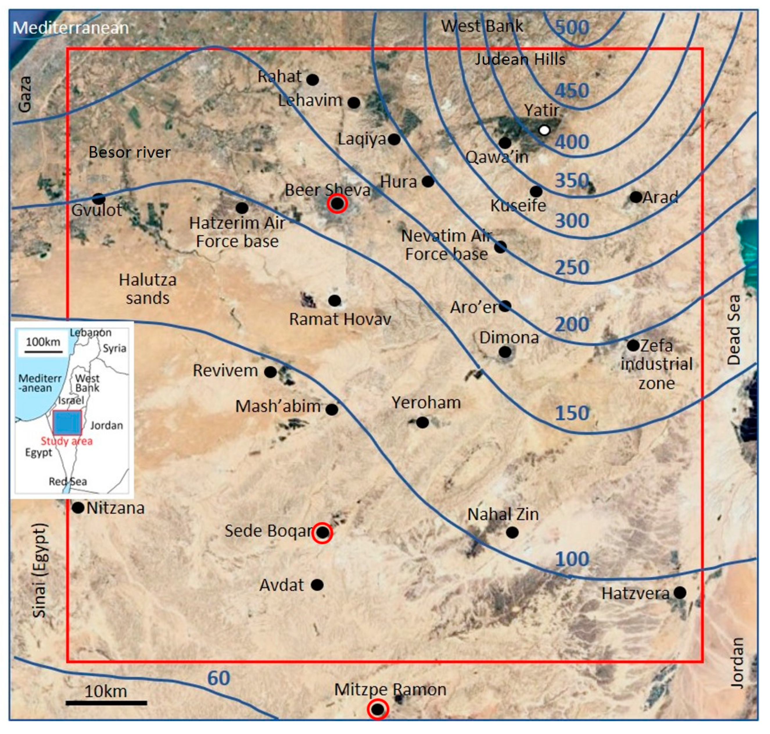
The study was carried out in the northern margins of the Negev desert, across the ecotone formed by the transition between barren desert to the south and semi-arid, vegetated land to the north (Figure 1). Dryland ecosystems are important for many reasons, for example, they have emerged as key drivers of variability in global land CO2 uptake [4]. The Negev region is representative of drylands in large areas of Western Asia and North Africa (WANA) which share the same physical environments, including low precipitation and a similar range of soils and topography. Also, there are similarities in land uses such as pastoralism, rain-fed and irrigated cropping, informal settlements, and some urban and industrial areas. The Negev provides a convenient example of a dryland ecotone since the width of the environmental gradient is approximately 80 km north to south, whereas, for example, the same zone in parts of Niger extends over approximately 173 km and in Western Australia 632 km.

Figure 1.
The 80 × 80 km study area in the northern Negev, Israel, showing the gradient between vegetated land (grey) in the north and barren desert (tan) in the south. The only rainfall stations making routine measurements in and near the study area are ringed in red. Locations mentioned in the text are shown. Isohyets (mm) were calculated from TRMM data (see Materials and Methods). Background satellite image from Google Earth, inset map modified from Geolounge.
Precipitation in the northern Negev ranges approximately from 50 to 250 mm per year and aridity from 0.203 to 0.124 [5]. In each year there is a brief period of rainfall followed by a more prolonged dry period, but the totals vary strongly from year to year. The low rainfall totals are somewhat alleviated by two factors; the climate is Mediterranean in which precipitation falls mostly in winter when insolation and evapotranspiration are lowest [6] and, second, there is a significant input of water in dew which can exceed rainfall in some places [7,8,9,10].
The correlations of four environmental factors with net primary production (NPP) were calculated: precipitation (P); land cover and land use (L); topography (T); and interannual variation (V) of NPP. This last property was included since it can be a critical factor affecting vegetation independent of precipitation [11,12] but is not captured in long-term, climatological statistics. To detect interannual differences in other factors, the year of observation (Y) was included. Note that the names and abbreviations of the variables used are capitalized throughout the text to indicate they are defined classes, not simply descriptive. The significance of each of the environmental variables in relation to NPP was examined using multiple linear regressions to isolate effects of individual variables and their component categories in the presence of variation of all four factors.
As in most sparsely populated arid areas, there is a paucity of continuous, long-term environmental measurements. For the Negev, there were few suitable, existing data sets and so they were developed for this study using other, available sources. It is not uncommon for environmental factors to affect NPP in different ways at more than one spatial scale, for example, precipitation is relevant at both climatological and local scales. The scale of interest in this study was approximately 1 ha, so NPP was calculated from Landsat 30 × 30 m data.
2. Materials and Methods
2.1. Study Area
The study region was an 80 × 80 km area in the northern Negev (Figure 1). Some types of land cover or land use were not of interest, including informal habitation, urban, buildings, water bodies, and rivers. These were excluded using the land cover map developed in this study. Narrow, low-order drainage systems and associated riparian strips that are the result of runoff were masked by coincidences of flat, well-vegetated, narrow, linear areas. Elevations >600 m above sea level were also excluded because of their local, orographic rainfall patterns. A one-pixel buffer was added to each masked feature to reduce the effects of inaccuracies in the land use maps and radiometric contamination by neighboring pixels.
2.2. Environmental Factors
Maps of the environmental factors were developed as part of the study since existing data do not show these features or scales are too coarse. Other, potentially important variables, such as local soils could not be included owing to a lack of spatially continuous data or adequate resolution.
2.2.1. Precipitation (P)
In the absence of a more appropriate measures for plant available water, total annual precipitation was used. Unfortunately, there are only two Israel Meteorological Service rainfall stations in the study area and a third 12km to the south (Figure 1). While rainfall has been measured in additional sites, none had records for the entire study period. Clearly, so few stations were inadequate to map precipitation. Therefore, annual totals were estimated by summation of daily Tropical Rainfall Measuring Mission (TRMM) 3B42 data [13] for each of 10 years (2000–2009). TRMM data have 0.25° × 0.25° (28 km at the study site) resolution which was rescaled to 30 m using cubic convolution. It should be noted, however, that TRMM does not include dew, which can be a significant source of soil moisture. Ten classes differing by 50 mm were defined.
2.2.2. Land Cover and Land Use (L)
A land cover map was created using multitemporal Landsat data, combined with land-use maps to capture features that are not spectrally distinct. Long-term climate records of rainfall in southern Israel were used as surrogates for the dates of three stages in the growing season: pre-onset, peak, and post-winter. Landsat 7 ETM+ channel 3 (630–690 nm) and 4 (775–900 nm) surface reflectance data for the three seasons in three years (2001, 2002, 2003) were classified with an ISODATA unsupervised classifier, set to a maximum standard deviation of 1.0, minimum cluster size of a single pixel, maximum of 1000 iterations, and a threshold change between iterations of 5.0%. Five classes were produced, subsequently found to relate to perennial vegetation on soil, shrubs on dark soil, exposed dark/red soil, sandy sheet soils, and bare/rocky surfaces. Finally, the five classes were combined with land-use maps [14,15] using a decision tree classifier. Small classes of less than 500 pixels were fused with the most similar, larger class, to make 10 land cover classes.
2.2.3. Topography (T)
Shuttle Radar Topography Mission (SRTM) elevation data with 30 m postings and finer than 10 m vertical resolution were used to map slope and aspect. Slope was divided into three ranges: flat (<1%); shallow (1–10%); and steep (>10%). Aspect was divided into two classes, N (270°–44°) and S (45°–269°). Slope and aspect were then combined into five overall topography classes: flat; N-facing and shallow; N-facing and steep; S-facing and shallow; S-facing and steep.
2.2.4. Interannual Variation (V)
The standard deviation of NPP in each Landsat pixel was calculated and averaged for the 11 years of the study. Five equal interval classes were defined.
2.3. Land Capability Classes
In order to reveal the effects of the selected environmental factors on NPP, areas that were minimally affected by other factors were identified. This was performed using the Local NPP Scaling method [3] in which Land Capability Classes (LCCs) were created by selecting areas in which all four environmental variables were in the same range. This segmentation is based on the concept of land units, a fundamental component in landscape ecology [16,17]. Each variable was divided into different numbers of classes: P 10; T 5; C 10; and V 4 (Table 1). These were then combined by intersection. Thus, the theoretical number of unique LCCs was 2000 for each of 11 years. However, not all combinations occurred, and LCCs with <500 pixels were fused with their most similar class, resulting in a total of 343 × 11 years = 3773. Analyses were conducted on LCC values as well as their individual, constituent pixels.

Table 1.
Percentage of pixels in the classes of each independent variable. Note differences in the number of classes between the four variables and some empty land cover classes.
2.4. Net Primary Production
NDVI was calculated using Landsat 5 ETM+ bands 3 (630–690 nm) and 4 (750 to 900 nm). Two scenes were needed to cover the study area (Path 174, Rows 38 & 39). A slight mismatch at the boundary (<10 pixels) was filled with the averages of pixels either side. Growing-season total NDVI was converted to NPP by regression with NPP from MODIS MOD17A3 [18]. This MODIS product has 1 km2 resolution—approximately 11 times coarser than Landsat—and therefore finer differences were obtained by interpolation. Furthermore, MOD17A3 does not cover all the study area, so the calibration had to be made at the northern margin of the Landsat data. The observed NPP measured using Landsat is referred to as “NPPobs” throughout the text.
Landsat is not ideal since the 8-day gap between satellite overpasses and data losses caused by clouds and haze that can result in missed parts of a growing season: this was especially problematic owing to the brevity of the growing season in the drier areas. Therefore, a single, best quality, Landsat acquisition nearest to the peak of the growing season was used for each year, the date determined from daily MODIS MOD17A3 NDVI data. Clearly, a single measurement cannot provide annual totals, and so the errors of using single Landsat scenes were examined by comparison with annual totals derived from MODIS and other parameters of the growing season.
2.5. Regression of NPP on Environmental Variables
Regressions were calculated for each of the environmental (independent) variables individually. Two additional regressions were included that combined all the variables and all except precipitation, in the expectation that precipitation would be the principal independent variable and would dominate a combined regression. The significance of each individual and combined regressions were assessed with the regression F statistic and the proportion of the variance accounted for with r2. The significances of the individual classes within each categorical independent variable were then examined using the regression coefficients.
2.6. Summary of Processing Steps
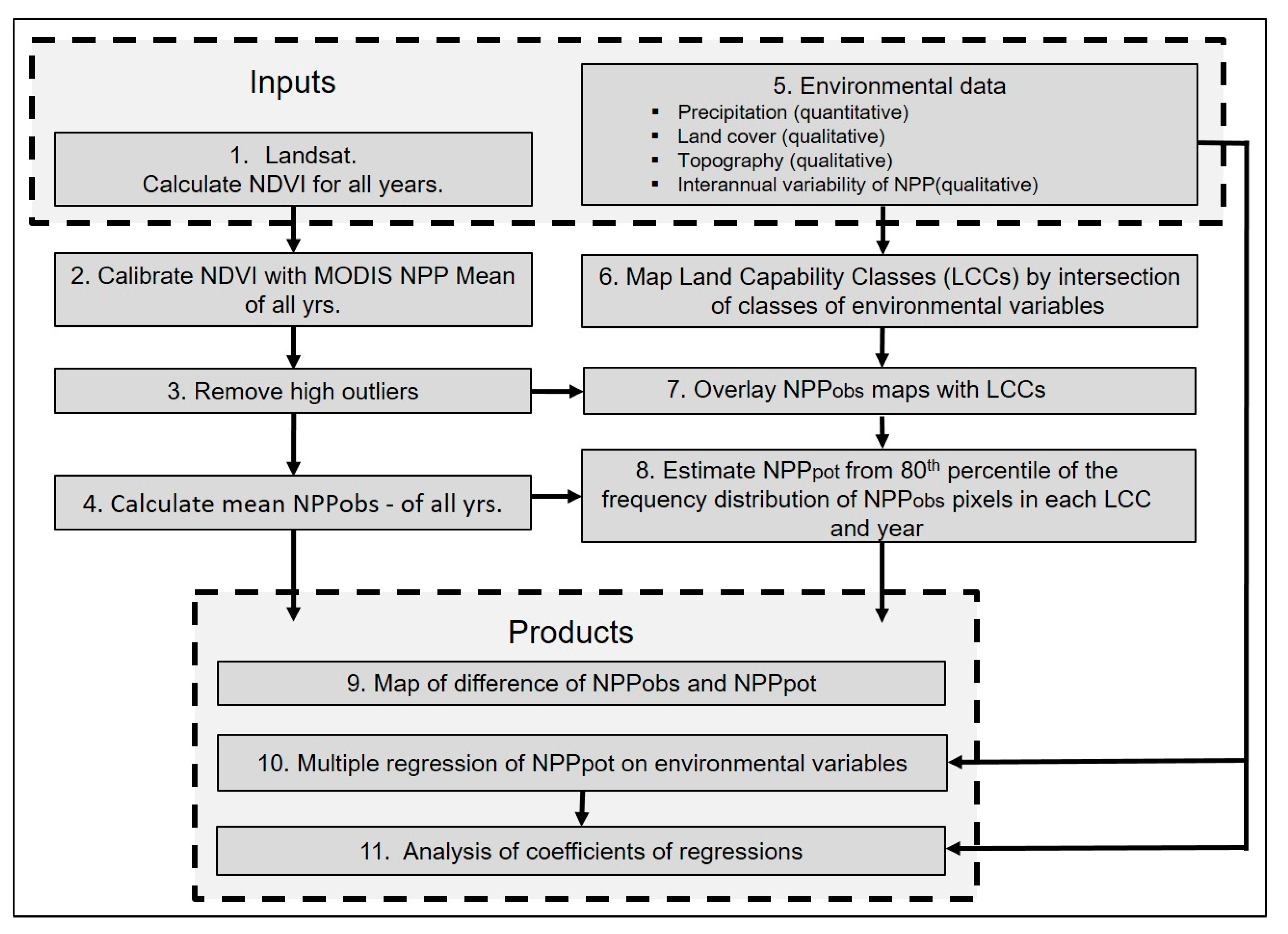
The steps from raw satellite and environmental data inputs to the final products—the difference between NPPpot and NPPobs, regression of NPPpot on environmental variables and the analysis of regression coefficients—are summarized in Figure 2.
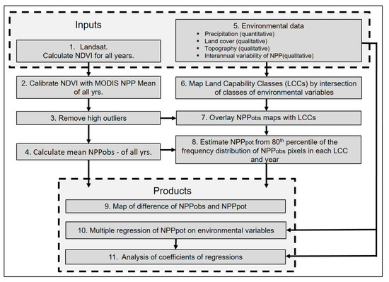
Figure 2.
Schematic diagram of data processing steps. Boxes 1 and 5 show the data inputs and boxes 9 to 11 the products used in the analyses.
3. Results
3.1. Environmental Variables
3.1.1. Precipitation (P)
The 11-year average precipitation had a predominant N to S gradient, from >200 to <30 mm (Figure 1). This was somewhat modified in the NE—presumably an orographic effect of the greater elevation of the southern tip of the Judean hills. The mean N-S gradient in the TRMM map was 3 mm/km, somewhat lower than Goldreich [19] (5 mm/km). While the annual precipitation of the TRMM grid cells values varied between years, it is important for this study to note that, in each year, their relative values and geographical patterns were very similar. The TRMM-derived isohyets were similar to data at individual stations in the study area [19,20].
3.1.2. Land Cover and Land Use (L)
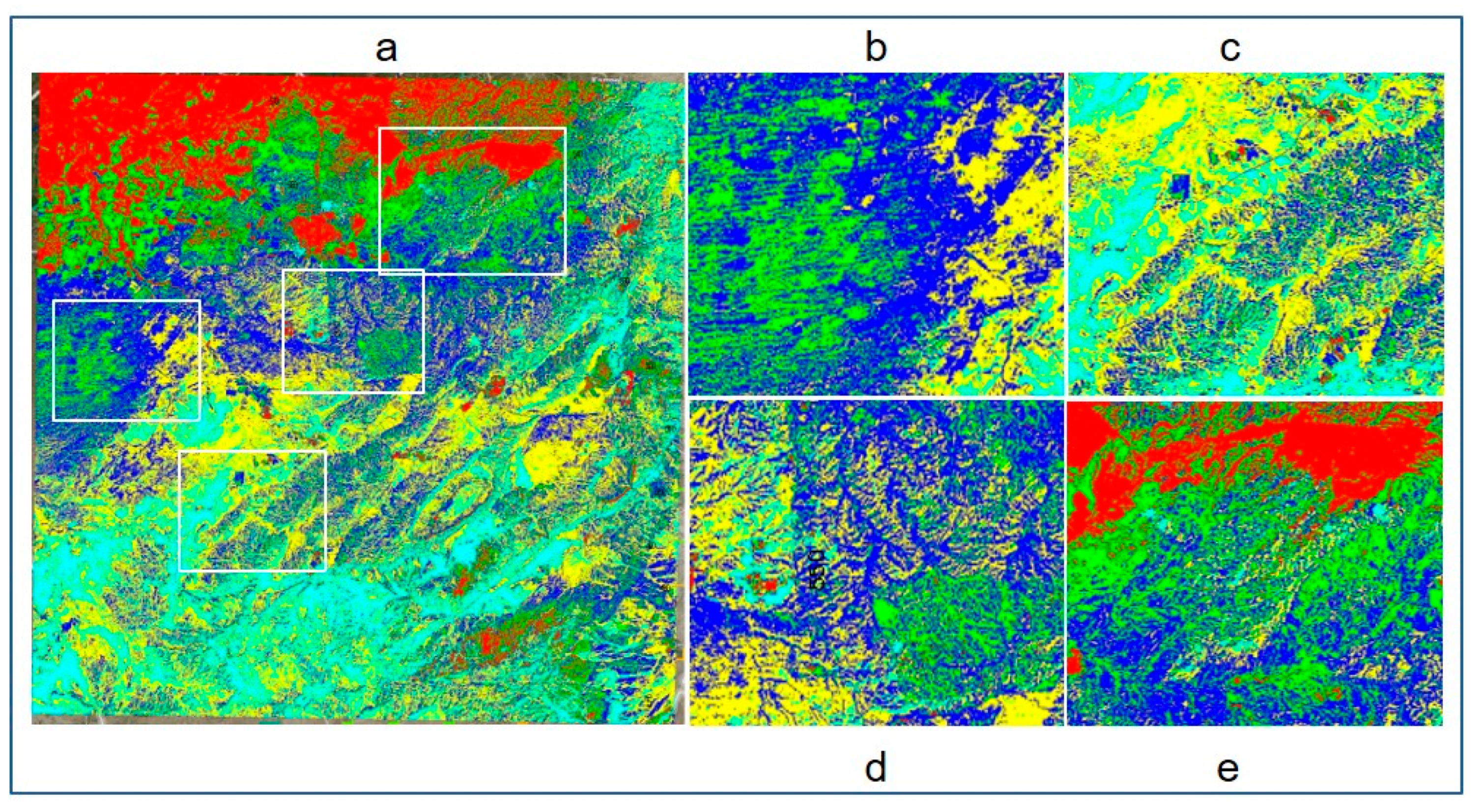
There was a strong correlation of land cover with the precipitation gradient (Figure 3), but large areas of other surfaces complicated this pattern. The zonal pattern is obvious at the lower resolution (Figure 3a), but at higher resolutions (Figure 3b–d) many finer scale variations were evident.
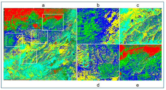
Figure 3.
Land cover and land use map from classification of multitemporal Landsat data and land use maps. (a) Entire study area (see Figure 1 for scale); (b) dunes on the Halutza sand sheet; (c) topographic variation; (d) local variation in vegetation cover; (e) dense forest, savannization, and dryland farming. Color codes: red, perennial vegetation and towns; blue, sandy vegetated; cyan, exposed dark, red soils, hilly drainage; dark green, sand sheet; light green, dryland agriculture; and yellow, bare/rocky surfaces. A digital file of this image is available from the corresponding author.
3.1.3. Topography (T)
The SRTM90 analysis indicated a gradient across the study area, dividing the coastal plain to the NW from more broken terrain, particularly to the SE at the edge of the Jordan valley. Large differences in slopes generally increased from NE to SW. Aspect had strong, fine-scale variation throughout. There were some slight regional patterns in which W aspects were more frequent in the west and E aspects in the east. At the finest scale, features such as dunes were detected (Figure 3b).
3.1.4. Inter-Annual Variation (V)
Variability increased from S to N, correlated with the gradient of low rainfall in the desert to the higher rainfall area in the N. The greatest variability was on cultivated land in the NW, where land cleared between crops and intermittent irrigation probably caused by extreme variation in vegetation cover.
3.2. Land Capability Classification
The map of land capability classes (LCCs) was strongly influenced by the coherence of the precipitation zones. Different values of the other environmental variables were generally scattered over the entire study area. Most LCCs consisted of several, spatially-separated polygons. There were 45 LCCs after fusion of smaller classes.
3.3. Landsat Measurements of Annual NPP
In each year the dates of the Landsat acquisitions were different - from day 19 to 141. However, they captured most aspects of the spatial variation in MOD13Q1 NPP. Landsat NDVI and peak daily MOD13Q1 NPP (Figure 4) were linearly related. The main differences were in the regression constants, while the coefficients were more stable across years (Figure 4), indicating that the relative NPP values within years were more constant in spite of differences in actual values of individual years. Since the purpose of this study was to make spatial comparisons, the interannual differences were of less consequence. Nevertheless, the patterns of NPP may have changed with seasons, so interannual geographic comparisons may sometimes have been inaccurate.
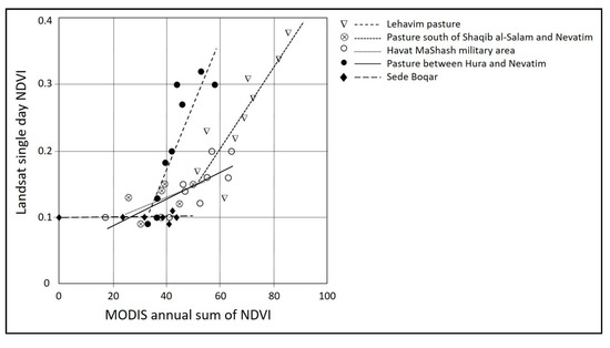
Figure 4.
Comparison of the annual sum of NDVI from MODIS MOD13Q1 with the single-day, per year Landsat values.
3.4. NPP of Study Area
3.4.1. Geographical
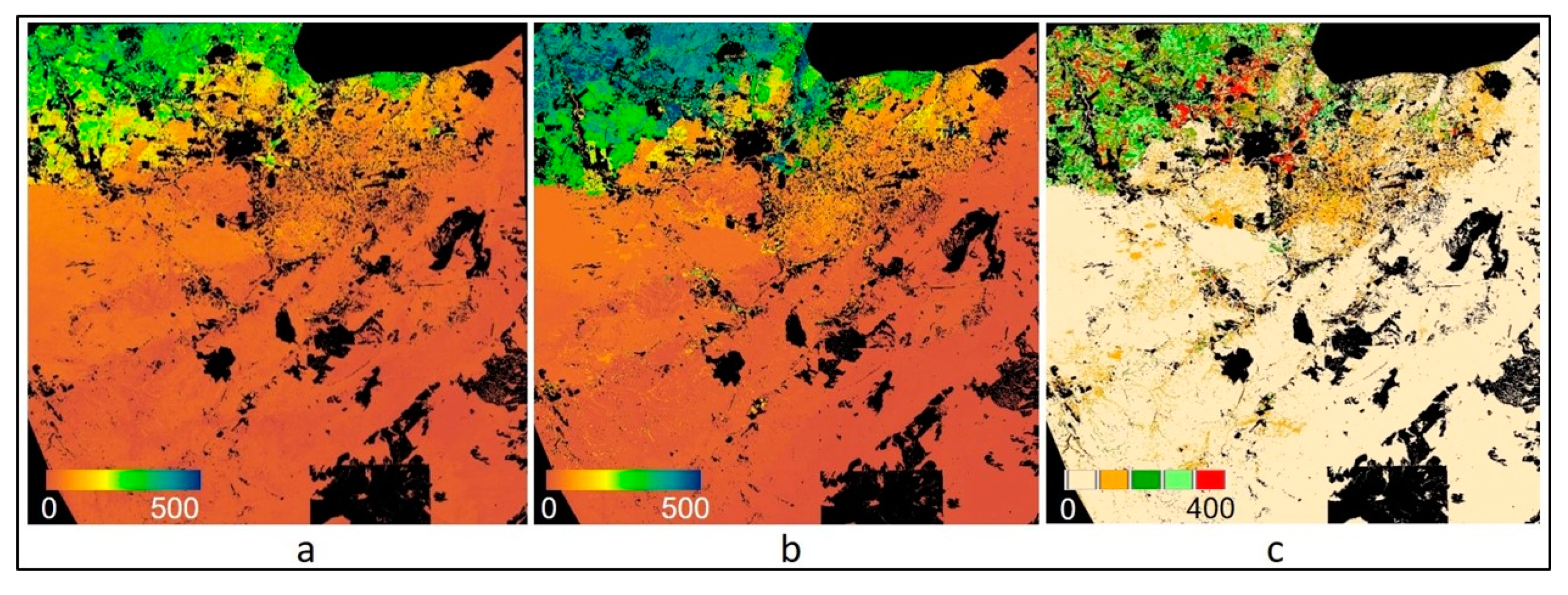
The 12-year mean NPPobs (Figure 5a) shows the anticipated strong influence of the pattern of rainfall (Figure 1). There were distinct geographical variations associated with differences in land surface conditions and human utilization [21]. The NPP of the 45 LCCs were low in the arid S and high in the N where there was cultivation, irrigation and fertilized fields. The strongest relationship with precipitation was in the middle range of values, as expected, since the lowest was largely in the arid S region and the highest in the more limited part of the study area in the N.

Figure 5.
NPP of the study area from Landsat. (a) NPPobs direct from Landsat data; (b) potential NPP (NPPpot); (c) difference between NPPobs and NPPpot. Means for 2001–2010 and 2012, all in gCm−2 yr−1. Large area masked at the S margin was caused by unknown category in the NGI land use map. Digital files of these images are available from the corresponding author.
3.4.2. Significance of Environmental Variables
All regressions on NPPpot were more significant than on NPPobs (Table 2), at both the individual pixel (Table 2a) and the land capability class (LCC) level (Table 2b). For the pixel and LCC levels, the multiple regressions including all variables but omitting P of both NPPobs and NPPpot, were very slightly more significant than with P included. Amongst the regressions on individual explanatory variables, V had the highest significance in both NPPpot and NPPobs—from 1.57 to 4.84 times. At both the pixel and LCC levels, the ranking of significance of independent variables were the same, except for L at the pixel level. T and Y had by far the lowest significance in both levels.

Table 2.
Multiple regression results for NPPobs and NPPpot on seven combinations of environmental (independent) variables, together and singly, and for both the pixel (a), and land capability (b) classes. Higher F values show that a regression model provided a better fit to the NPP data than a model without the independent variable. Probability values were all significant at the 0.01% level (indicated by ***). r2 indicates the proportion of variation of the dependent variable that the regressions explain. Ranking of F and r2 is by magnitude, from highest to lowest. Variable names: V—Variation; P—Precipitation; L—Land cover; T—Topography; Y—Year of observation.
r2 values indicated that the regressions on NPPpot all accounted for a higher proportion of variation than for NPPobs, both at the pixel and LCC levels. The ranking of r2 values, although almost the same for NPPobs and NPPpot at both the pixel and LCC levels, differed from the F ranking.
3.4.3. Significance of Categories within Environmental Variables
The significances of the individual levels within each independent variable are indicated by their regression coefficients and probabilities of significance (Table 3 and Table 4).

Table 3.
Coefficient values for each category of regressions on NPPpot at the pixel level. Values represent the mean change in the response given a one unit change in each category of the independent variable. The larger the coefficient the greater the explanatory power of the category. Negative values indicate inverse relationships. Probability values were all significant at the 0.01% level (indicated by ***). Dark fill—coefficients >1000; medium fill—100–999; no fill—<100. All were highly significant.

Table 4.
Coefficient values for each category of regressions on NPPpot at the LCC level. Values represent the mean change in the response given a one unit change in each category of the independent variable. The larger the coefficient the greater the explanatory power of the category. Negative values indicate inverse relationships. Coefficients at the 0.01% probability level are indicated with 3 stars (***) and those not significant at the 5% level by NS. Dark fill—coefficients >1000; medium fill—100–999; no fill—<100.
At the pixel level, all independent variable categories made significant contributions to their regressions. In the combined regression and the combined with P omitted, the categories that made large contributions were V, especially categories V3 and V4, and to a slightly lesser extent L8 (planted forest). The L categories L2 (cultivation in the N) and L9 (bushes in dry valleys throughout) were moderately large. V2 was also large, so all V categories made big contributions to the overall regressions. Some coefficients were negative: T2 and T4 (low slope to N and S); L3 (sand sheet); and in six of the Y years.
In the regressions on individual independent variables, those with higher coefficients in the combined regressions were also very high alone; to which were added T3 and T5 (steep N and S) and L2 (cultivated in the N). Other categories that were moderately large were the remainder of T classes (T2, T4), and the remainder of the L classes (L3, L4, L9) with the exception of L10 (colluvium). Most negative coefficients in the combined regressions were also negative in the individual ones. Individual years (Y) oscillated between negative and positive values.
At the LCC level, as at the pixel level, there were large coefficients for V, especially categories V3 and V4, and to a lesser extent L2 and L8. Among the moderate values other similarities with the pixel level were in V2, T3, T5, L2, L9, P, and Y2005, 2006, and 2008–2012. L10 was added to the moderate coefficients but was smaller in the pixel level. Each variable apart from V had one or more insignificant coefficients. The main difference between the pixel and LCC levels was the number of insignificant coefficients, 72 in the pixel and 25 in the LCC level.
4. Discussion
4.1. Methodology
The aim of calculation of NPPpot from the observed satellite data was to avoid the uncertainties caused by confounding with unknown environmental and other factors. Alternative methods for establishing NPPpot are possible, for example [22] used a water balance model. That approach has the advantage of excluding any confounding variables since it uses only external weather data. However, derivations of NPPpot that are more complex than the light use efficiency model in MOD17A3 (used here for calibration of Landsat) are limited by the availability of the model inputs. For example, a candidate model might be Biome-BGC [23], however it requires approximately 44 input variables and the same number of parameters—quite unrealistic for remotely-sensed, spatially continuous studies. Even the much simpler water balance model [22] requires detailed weather data but these ground data are often inadequate, for example in the Negev study area (6400 km2) there were only two meteorological stations.
The accuracy of the estimation of NPPpot using LNS could be affected by various factors. An unavoidable one is when an LCC contains no pixels at the potential, in which case there would be an underestimation. Some significant enhancements of the technique are possible. For example, homogeneity of environmental factors within each LCC is a basic requirement and this could be improved with better land capability classification, for example, by using more independent variables, higher spatial resolution remote sensing, and some newly developed remote sensing techniques [4].
An important drawback in this study of the Negev is the low temporal repeat frequency of Landsat data, which could not capture the full progress of the growing season and therefore could be poor estimates of values for the entire growing seasons, especially since the season can last only for weeks in some of the more arid areas. The different stages of the growing seasons at which the Landsat data were available meant that the data were better suited to comparisons of responses of NPP to environmental factors at the time of the acquisition rather than entire growing seasons. Techniques exist, such as STARFM [24], that match sensors of different frequencies and resolutions, but there were inadequate data to apply such methods in this study. Temporal frequencies of multispectral remote sensing data are improving with newer sensors, for example, the Landsat-Sentinel-2 virtual constellation [25]. This combination has frequencies of about 2.9 days and similar spatial resolution to Landsat [26]. Sentinel-2 data started in 2015, but do not yet provide an adequate time-series to resolve the large inter-annual variations in drylands.
4.2. NPP of Cover Types
The maps of NPP indicated that there was a range of NPPpot from 0 to 500 gm−2 yr−1 (Figure 5). The highest in was in the Aleppo pine plantations in the N on the edge of the Judean hills, also in irrigated fields in the NW and scattered small areas of irrigation in the desert. The extensive woodlands planted in the JNF savannization program varied in NPP, presumably because areas are continuing to be added where the NPP can be expected to initially drop with removal of native vegetation creating bare ground, and thereafter a slow regrowth towards the long-term, low NPPpot typical of disturbed land. Overall, most of the land in the drier areas had low NPPpot, lowest for colluvium, followed by rock and sand.
The precipitation gradient was NE to SW but the NPPpot gradient was from NW to SE. This pattern correlates with the locations of more fertile soils and average but not the highest precipitation in the NE of the study area. However, one aspect of precipitation that could not be addressed in this study was dewfall, which has been noted to contribute 48% of the annual precipitation in one site in the study area [27] and as much as 63% of soil moisture used by some plant species [28].
Overall, NPPpot was approximately 50% lower on steep compared with shallow slopes, but there were no consistent differences between N and S aspects. Slopes that receive higher insolation in this region are known to have different vegetation and to affect production [29]. Furthermore, dew is correlated with slope and aspect [9] and may account for some of the effects of the T variable.
Interannual variation (V) in NPPpot was greater in the wetter sites where P was highest. A correlation of V with P, although low (r2 = 0.2) was highly significant. This correlation led to higher levels of significance in regressions that included V as well as P (Table 2, Table 3 and Table 4). Since V is mainly a result of interannual variation in P, it could therefore be used as an indicator of variation over a representative run of years. An advantage would be that, since V is measured for each 30 m pixel, it could provide a much finer geographical resolution of ground water status than precipitation from TRMM (28 km).
4.3. Regional C Sequestration
Independent measurements of NPP relevant to southern Israel were obtained by analysis of two available field reports [30,31] and also two global maps [18,32] (Table 5). The NPPpot values calculated in the present study were in the same range. Non-forest was somewhat lower, possibly because the present study included a large area of desert. Differences may also have been partly a result of the higher resolution of Landsat which allowed much greater discrimination of fine variations in the environment.

Table 5.
Comparison of potential NPP (NPPpot) found in this study with four independent reports. Adjustments were made to the reported values by partition of total productivities into tree and non-tree components for those that did not distinguished the two, and conversion from biomass to carbon units.
Several studies have suggested that grasslands may be carbon sinks or near equilibrium, and often shift between sources in drought years and sinks in other years (e.g., [33]). However, respiration was not measured here, so NEP was not available. Very low values of NPPpot occurred in some years which, coupled with the presence of perennial species which have a strong respiration demand, could easily result in carbon losses. Overall, our findings indicate that NPP was strongly linked to both climate and land surface characteristics. The high degree of local variability we found in the area challenges interpretations of environmental controls at broader scales [4].
5. Conclusions
The comparison of methods for correlation of remotely-sensed observations of observed NPP and estimated potential NPP with specific environmental controlling factors demonstrated that there was an improvement when the individual pixel values were replaced with the potential NPP that would occur in the absence of other, unmeasured—often unknown—factors. For example, the comparison of regressions of observed and potential NPP on environmental variables (Table 2, Table 3 and Table 4) indicated a very large improvement. For pixel-scale regressions, F ranged from 2.52 × 10⁷ to 7.37 × 10⁴ (average 7.90 × 10⁶) and for the LCC scale, 2285 to 3 (average 884)—all highly significant. The application of this method to the northern Negev refined the relationships of precipitation, land cover, topography, and interannual variation with NPP. The anticipated dominance of precipitation was confirmed, but was shown to be qualified by the other, more local factors, especially interannual variation.
Author Contributions
Conceptualization, S.D.P.; Methodology, S.D.P. and H.J.; Formal analysis, S.D.P., H.J.; Writing—original draft preparation, S.D.P.; Writing—review and editing, S.D.P. All authors have read and agreed to the published version of the manuscript.
Funding
This research was partially funded by the United States Department of Agriculture Forest Service International Programs and by the University of Maryland.
Acknowledgments
We thank Diyang Cui who assisted with statistical analyses and Uriel Safriel who provided unpublished Israeli documents. We greatly appreciate the constructive comments from the all anonymous reviewers.
Conflicts of Interest
The authors declare no conflict of interest.
References
- Balaghi, R.; Tychon, B.; Eerens, H.; Jlibene, M. Empirical regression models using NDVI, rainfall and temperature data for the early prediction of wheat grain yields in Morocco. Int. J. Appl. Earth Obs. Geoinf. 2008, 10, 438–452. [Google Scholar] [CrossRef]
- Rishmawi, K.; Prince, S.D. Environmental and anthropogenic degradation of vegetation in the Sahel from 1982 to 2006. Remote Sens. 2016, 8, 948. [Google Scholar] [CrossRef]
- Prince, S.D. Challenges for remote sensing of the Sustainable Development Goal SDG 15.3.1 productivity indicator. Remote Sens. Environ. 2019, 234, 111428. [Google Scholar] [CrossRef]
- Smith, W.K.; Dannenberg, M.P.; Yan, D.; Herrmann, S.; Barnes, M.L.; Barron-Gafford, G.A.; Biederman, J.A.; Ferrenberg, S.; Fox, A.M.; Hudson, A.; et al. Remote sensing of dryland ecosystem structure and function: Progress, challenges, and opportunities. Remote Sens. Environ. 2019, 233, 111401. [Google Scholar] [CrossRef]
- Trabucco, A.; Zomer, R.J. Global Aridity Index (Global-Aridity) and Global Potential Evapo-Transpiration (Global-PET) Geospatial. Available online: https://cgiarcsi.community/data/global-aridity-and-pet-database/ (accessed on 2 September 2020).
- Nicholson, S.E. Dryland Climatology; Cambridge University Press: Cambridge, UK, 2011. [Google Scholar]
- Jacobs, A.F.G.; Heusinkveld, B.G.; Berkowicz, S.M. Dew measurements along a longitudinal sand dune transect, Negev Desert, Israel. Int. J. Biometeorol. 2000, 43, 184–190. [Google Scholar] [CrossRef]
- Kidron, G.J.; Yair, A.; Danin, A. Dew variability within a small arid drainage basin in the Negev Highlands, Israel. Q. J. R. Meteorol. Soc. 2000, 126, 63–80. [Google Scholar] [CrossRef]
- Kidron, G.J. Angle and aspect dependent dew and fog precipitation in the Negev desert. J. Hydrol. 2005, 301, 66–74. [Google Scholar] [CrossRef]
- Zangvil, A. Six years of dew observations in the Negev Desert, Israel. J. Arid Environ. 1996, 32, 361–371. [Google Scholar] [CrossRef]
- Ward, D.; Saltz, D.; Olsvig-Whittaker, L. Distinguishing signal from noise: Long-term studies of vegetation in Makhtesh Ramon erosion cirque, Negev desert, Israel. Plant Ecol. 2000, 150, 27–36. [Google Scholar] [CrossRef]
- Ward, D.; Saltz, D.; Ngairorue, B.T. Spatio-temporal rainfall variation and stock management in arid Namibia. J. Range Manag. 2004, 57, 130–140. [Google Scholar] [CrossRef]
- Huffman, G.J.; Bolvin, D.T.; Nelkin, E.J.; Wolff, D.B.; Adler, R.F.; Gu, G.; Hong, Y.; Bowman, K.P.; Stocker, E.F. The TRMM Multisatellite Precipitation Analysis (TMPA): Quasi-Global, Multiyear, Combined-Sensor Precipitation Estimates at Fine Scales. J. Hydrometeorol. 2007, 8, 38–55. [Google Scholar] [CrossRef]
- Central Bureau of Statistics. National Geographic Information (NGI) Land-Use Layer; State of Israel: Jerusalem, Israel, 2007.
- Central Bureau of Statistics. National Geographic Information (NGI) Land-Use Layer; State of Israel: Jerusalem, Israel, 2002.
- Bunce, R.G.H.; Barr, C.J.; Gillespie, M.K.; Howard, D.C. The ITE land classification: Providing an environmental stratification of Great Britain. Environ. Monit. Assess. 1996, 39–46. [Google Scholar] [CrossRef]
- Zonneveld, I.S. The land unit-A fundamental concept in landscape ecology, and its applications. Landsc. Ecol. 1989, 3, 67–86. [Google Scholar] [CrossRef]
- Running, S.; Zhao, M. MYD17A3HGF MODIS/Aqua Net Primary Production Gap-Filled Yearly L4 Global 500 m SIN Grid V006. Available online: https://catalog.data.gov/dataset/modis-aqua-net-primary-production-gap-filled-yearly-l4-global-500m-sin-grid-v006 (accessed on 2 September 2020).
- Goldreich, Y. Temporal variations of rainfall in Israel. Clim. Res. 1995, 5, 167–169. [Google Scholar] [CrossRef]
- Ziv, B.; Saaroni, H.; Pargament, R.; Harpaz, T.; Alpert, P. Trends in rainfall regime over Israel, 1975–2010, and their relationship to large-scale variability. Reg. Environ. Change 2014, 14, 1751–1764. [Google Scholar] [CrossRef]
- Prince, S.D.; Safriel, U.; Karnieli, A. Impacts of Land Use on Negev Rangelands: An. Exploratory Study. Final Report to the Mid-East. Program., International Programs; United States Forest Service: College Park, MD, USA, 2013; p. 20742.
- Boer, M.M.; Puigdefábregas, J. Predicting potential vegetation index values as a reference for the assessment and monitoring of dryland condition. Int. J. Remote Sens. 2003, 24, 1135–1141. [Google Scholar] [CrossRef]
- Thornton, P.E. User’s Guide for Biome-BGC, Version 4.1.1. Available online: https://daac.ornl.gov/daacdata/model_archive/BIOME_BGC/biome_bgc_4.1.1/comp/bgc_users_guide_411.pdf (accessed on 27 August 2020).
- Gao, F.; Masek, J.G.; Wolfe, R.E.; Huang, C. Building a consistent medium resolution satellite data set using moderate resolution imaging spectroradiometer products as reference. J. Appl. Remote Sens. 2010, 4, 043526. [Google Scholar] [CrossRef]
- Li, J.; Roy, D.P.; Li, J.; Roy, D.P. A Global Analysis of Sentinel-2A, Sentinel-2B and Landsat-8 Data Revisit Intervals and Implications for Terrestrial Monitoring. Remote Sens. 2017, 9, 902. [Google Scholar] [CrossRef]
- Claverie, M.; Ju, J.; Masek, J.G.; Dungan, J.L.; Vermote, E.F.; Roger, J.-C.; Skakun, S.V.; Justice, C. The Harmonized Landsat and Sentinel-2 surface reflectance data set. Remote Sens. Environ. 2018, 219, 145–161. [Google Scholar] [CrossRef]
- Evenari, M.; Shanan, L.; Tadmor, N. The Negev The Challenge of a Desert; Harvard University Press: Cambridge, MA, USA, 1971. [Google Scholar]
- Hill, A.; Dawson, T.; Shelef, O.; Rachmilevitch, S. The role of dew in Negev Desert plants. Oecologia 2015, 178, 317–327. [Google Scholar] [CrossRef]
- Sternberg, M.; Shoshany, M. Influence of slope aspect on Mediterranean woody formations: Comparison of a semiarid and an arid site in Israel. Ecol. Res. 2001, 16, 335–345. [Google Scholar] [CrossRef]
- Gelfand, I.; Grünzweig, J.M.; Yakir, D. Slowing of nitrogen cycling and increasing nitrogen use efficiency following afforestation of semi-arid shrubland. Oecologia 2012, 168, 563–575. [Google Scholar] [CrossRef] [PubMed]
- Helman, D.; Mussery, A.; Lensky, I.M.; Leu, S. Detecting changes in biomass productivity in a different land management regimes in drylands using satellite-derived vegetation index. Soil Use Manag. 2014, 30, 32–39. [Google Scholar] [CrossRef]
- Del Grosso, S.; Parton, W.; Stohlgren, T.; Zheng, D.; Bachelet, D.; Prince, S.; Hibbard, K.; Olson, R. Global potential net primary production predicted from vegetation class, precipitation, and temperature. Ecology 2008, 89, 2117–2126. [Google Scholar] [CrossRef]
- Zhang, G.G.; Kang, Y.M.; Han, G.D.; Mei, H.; Sakurai, K. Grassland degradation reduces the carbon sequestration capacity of the vegetation and enhances the soil carbon and nitrogen loss. Acta Agric. Scand. Sect. B Soil Plant Sci. 2011, 61, 356–364. [Google Scholar] [CrossRef]
Publisher’s Note: MDPI stays neutral with regard to jurisdictional claims in published maps and institutional affiliations. |
© 2020 by the authors. Licensee MDPI, Basel, Switzerland. This article is an open access article distributed under the terms and conditions of the Creative Commons Attribution (CC BY) license (http://creativecommons.org/licenses/by/4.0/).

