Mapping Canopy Chlorophyll Content in a Temperate Forest Using Airborne Hyperspectral Data


 ,
,  ,
, 
Abstract

1. Introduction
2. Materials and Methods
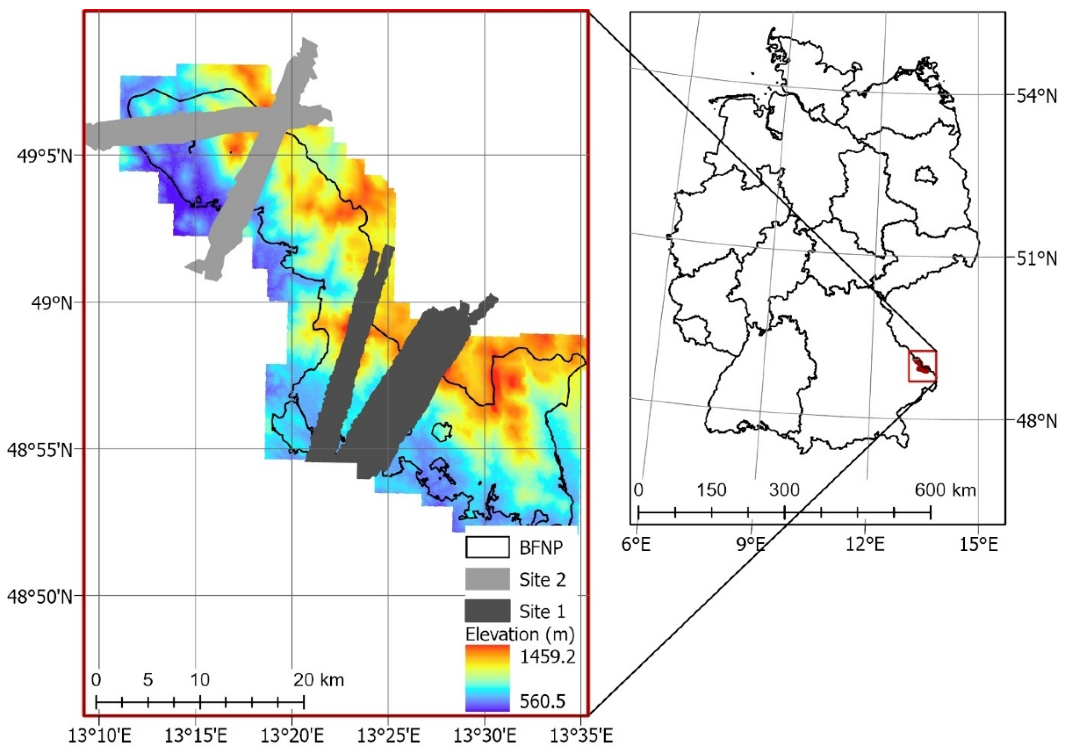
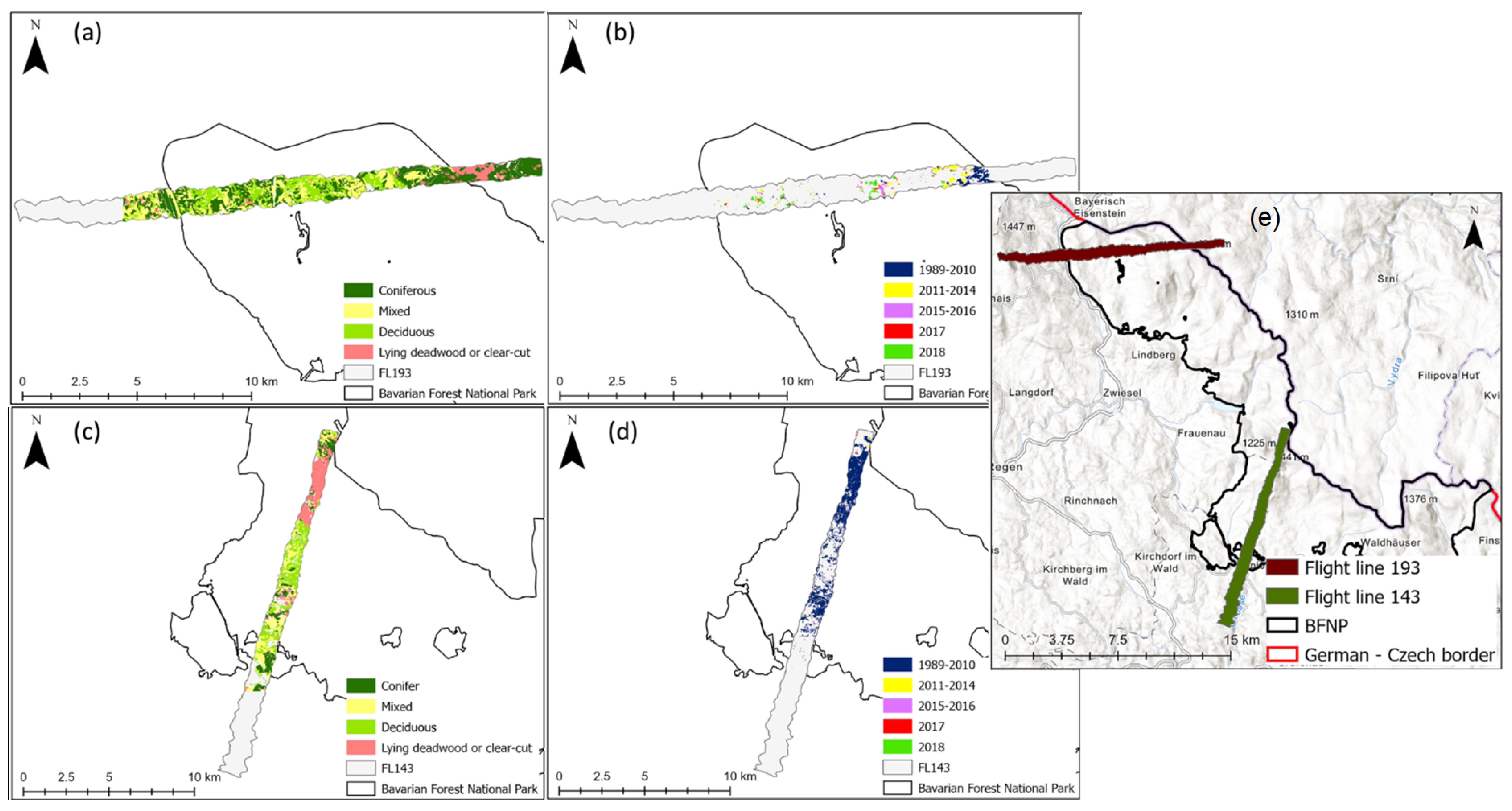
2.1. Study Site
2.2. Data Collection and Processing
2.2.1. Hyperspectral
2.2.2. Field Data
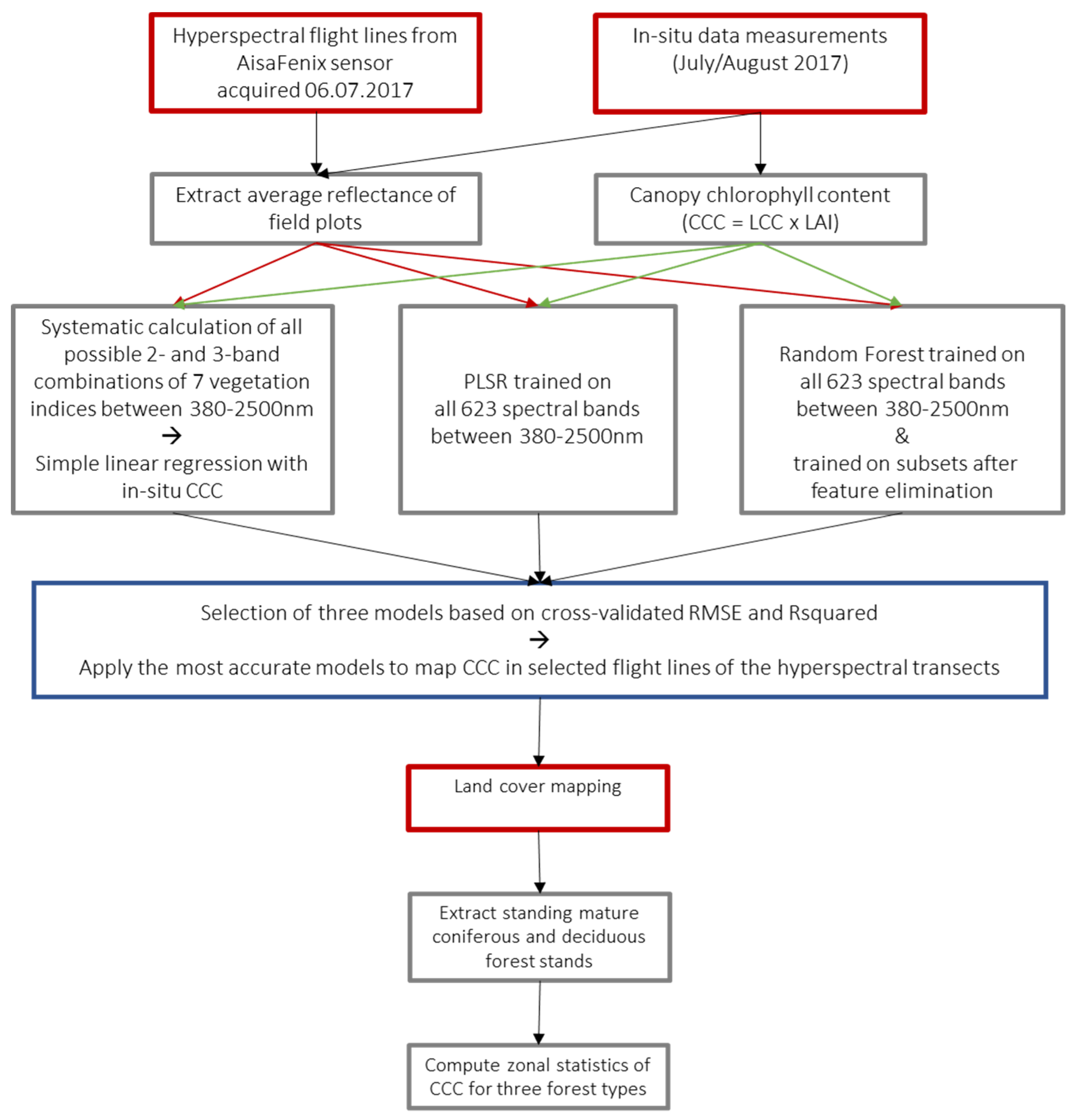
2.3. Methods
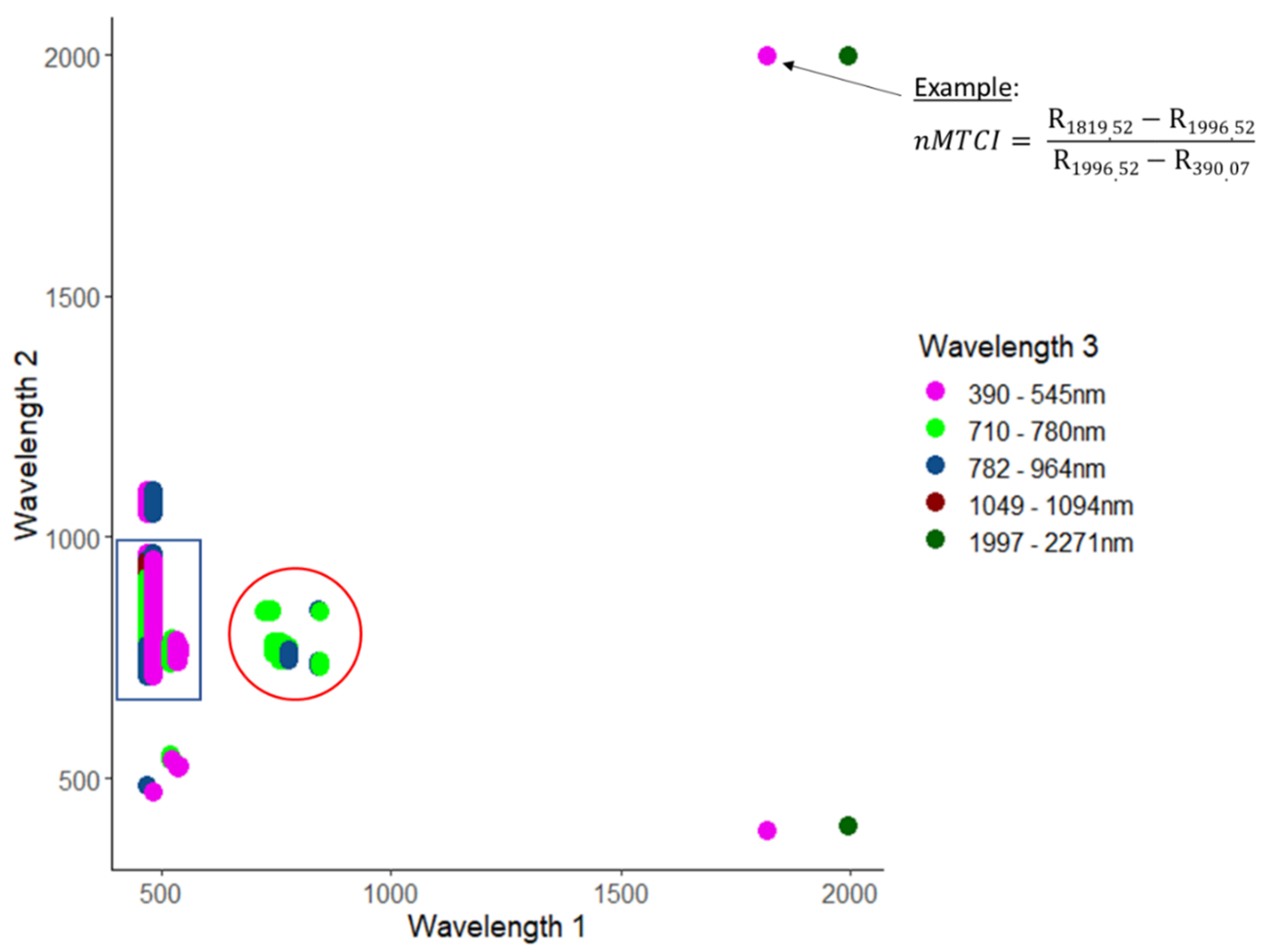
2.3.1. Hyperspectral Vegetation Indices
2.3.2. Regression Models for VIs
2.3.3. Partial Least Squares Regression
2.3.4. Random Forest
2.3.5. Validation
2.3.6. Mapping Canopy Chlorophyll Content
3. Results
3.1. Model Selection
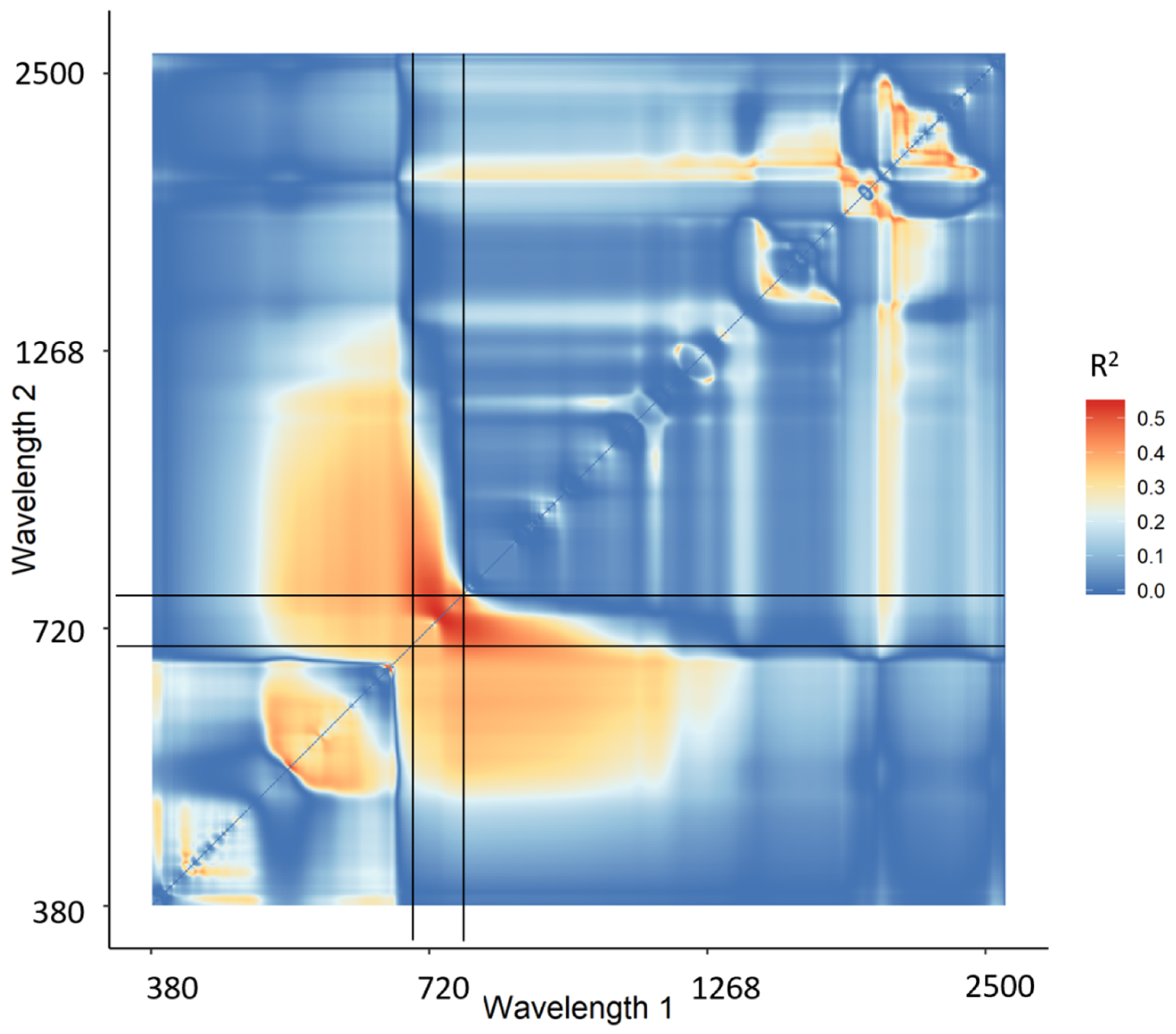
3.1.1. Narrowband Vegetation Indices
3.1.2. PLSR
3.1.3. Random Forest
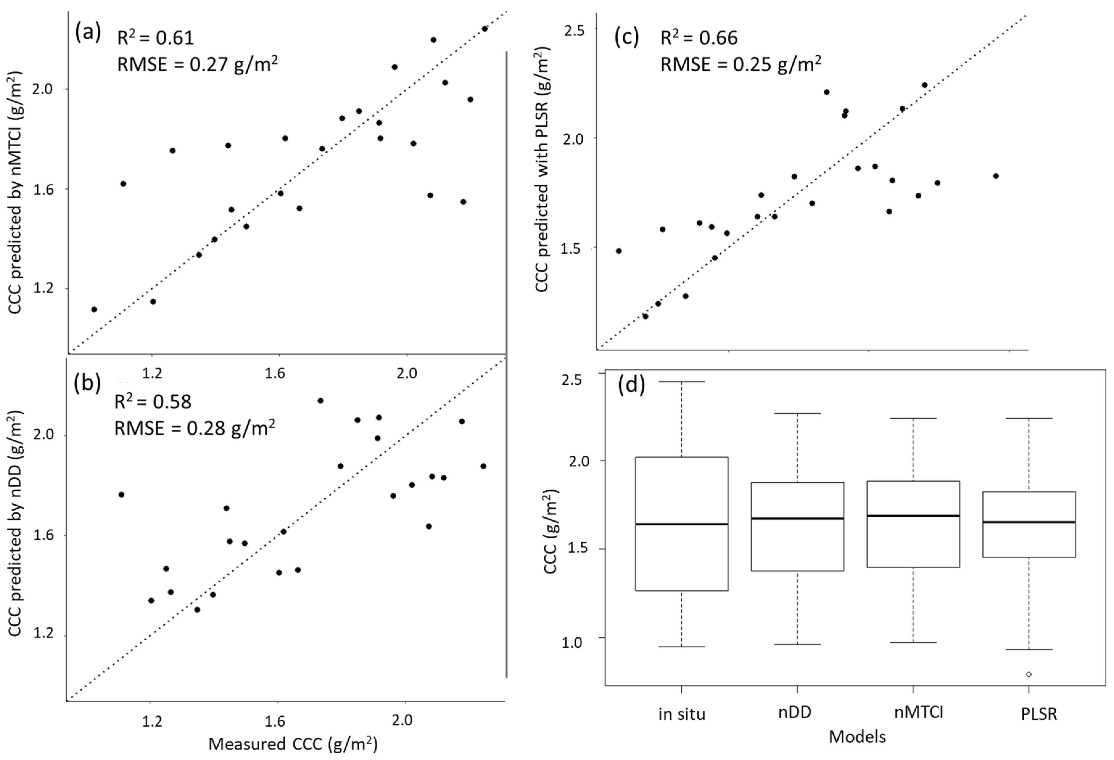
3.1.4. Model Comparison
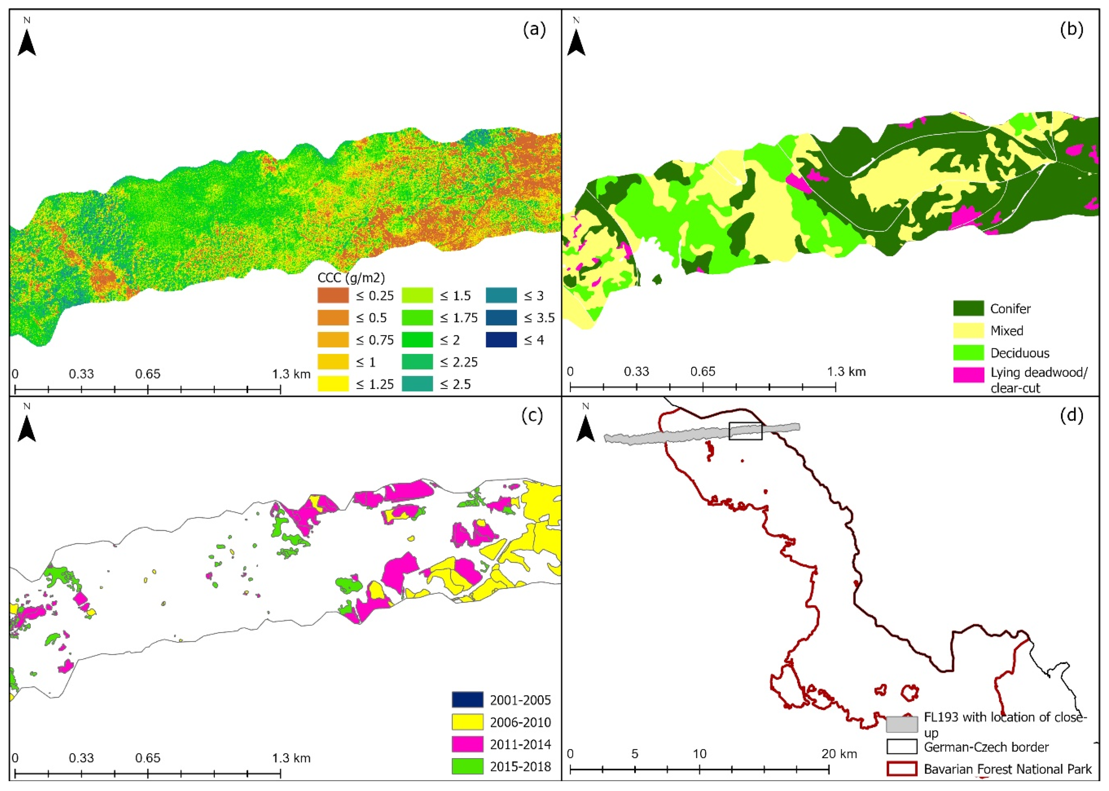
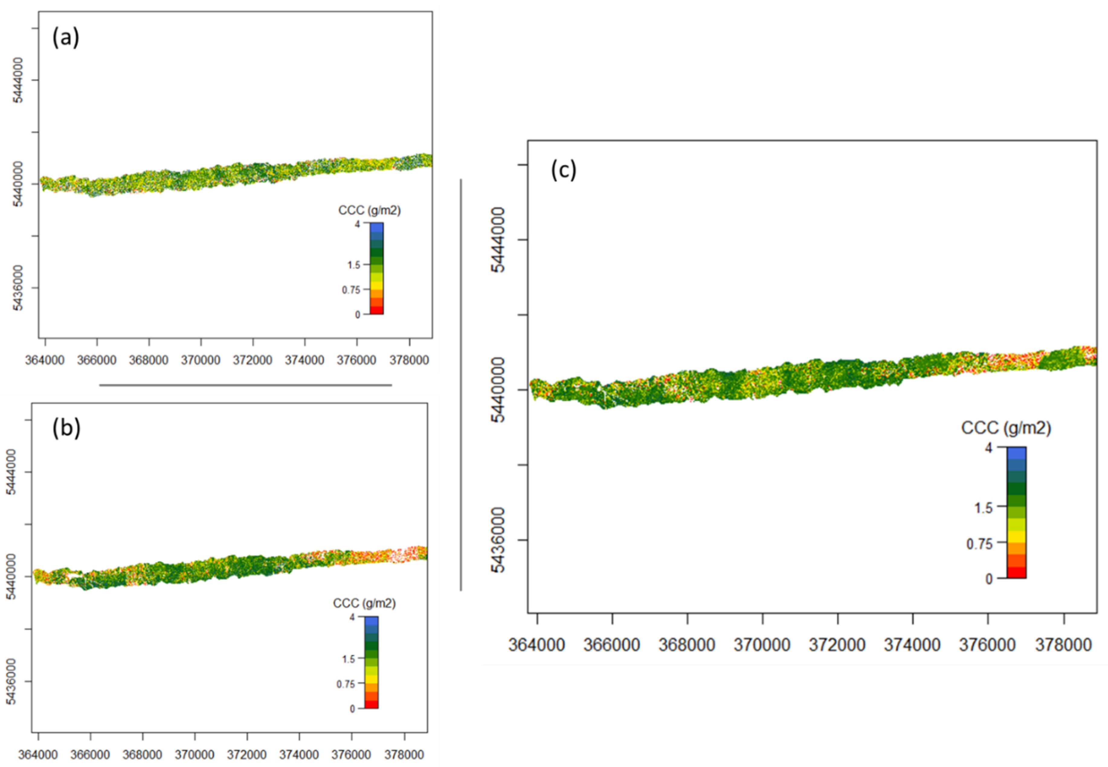
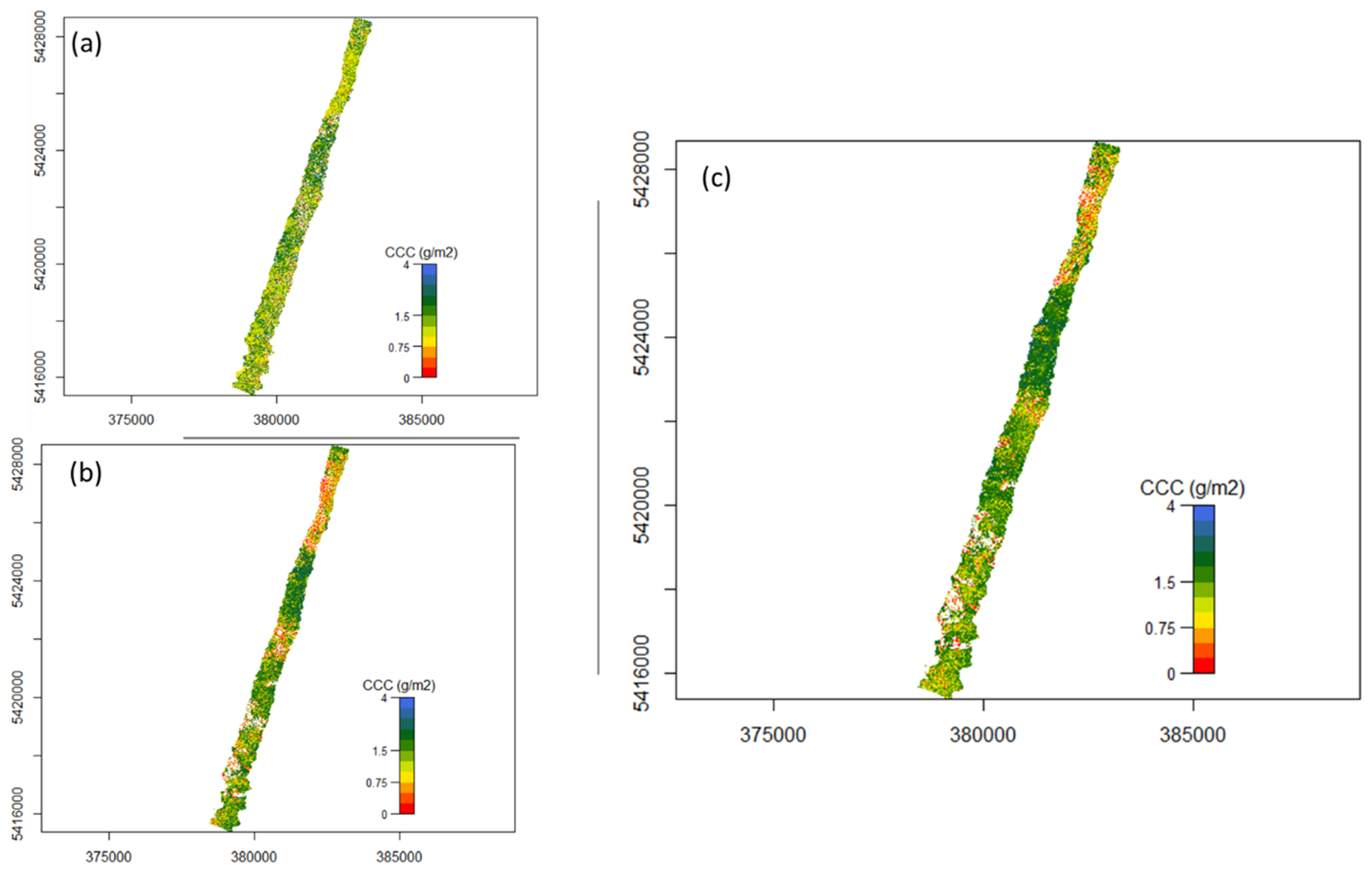
3.2. Mapping Canopy Chlorophyll Content
4. Discussion
5. Conclusions
Author Contributions
Funding
Conflicts of Interest
Appendix A


References
- Björkman, O.; Powles, S.B. Inhibition of photosynthetic reactions under water stress: Interaction with light level. Planta 1984, 161, 490–504. [Google Scholar] [CrossRef] [PubMed]
- Le Maire, G.; François, C.; Dufrene, E. Towards universal broad leaf chlorophyll indices using PROSPECT simulated database and hyperspectral reflectance measurements. Remote Sens. Environ. 2004, 89, 1–28. [Google Scholar] [CrossRef]
- Yang, X.; Yu, Y.; Fan, W. Chlorophyll content retrieval from hyperspectral remote sensing imagery. Environ. Monit. Assess. 2015, 187, 456. [Google Scholar] [CrossRef] [PubMed]
- Clevers, J.G.P.W.; Kooistra, L. Using Hyperspectral Remote Sensing Data for Retrieving Canopy Chlorophyll and Nitrogen Content. IEEE J. Sel. Top. Appl. Earth Obs. Remote Sens. 2011, 5, 574–583. [Google Scholar] [CrossRef]
- Inoue, Y.; Guérif, M.; Baret, F.; Skidmore, A.; Gitelson, A.; Schlerf, M.; Darvishzadeh, R.; Olioso, A. Simple and robust methods for remote sensing of canopy chlorophyll content: A comparative analysis of hyperspectral data for different types of vegetation. Plant Cell Environ. 2016, 39, 2609–2623. [Google Scholar] [CrossRef] [PubMed]
- Gitelson, A.A.; Keydan, G.; Merzlyak, M.N. Three-band model for noninvasive estimation of chlorophyll, carotenoids, and anthocyanin contents in higher plant leaves. Geophys. Res. Lett. 2006, 33. [Google Scholar] [CrossRef]
- Darvishzadeh, R.; Skidmore, A.; Abdullah, H.; Cherenet, E.; Ali, A.; Wang, T.; Nieuwenhuis, W.; Heurich, M.; Vrieling, A.; O’Connor, B.; et al. Mapping leaf chlorophyll content from Sentinel-2 and RapidEye data in spruce stands using the invertible forest reflectance model. Int. J. Appl. Earth Obs. Geoinf. 2019, 79, 58–70. [Google Scholar] [CrossRef]
- Skidmore, A.K.; Pettorelli, N. Agree on biodiversity metrics to track from space: Ecologists and space agencies must forge a global monitoring strategy. Nature 2015, 523, 403–406. [Google Scholar] [CrossRef]
- Pereira, H.M.; Ferrier, S.; Walters, M.; Geller, G.N.; Jongman, R.H.G.; Scholes, R.J.; Bruford, M.W.; Brummitt, N.; Butchart, S.H.M.; Cardoso, A.C.; et al. Essential Biodiversity Variables. Science 2013, 339, 277–278. [Google Scholar] [CrossRef]
- Homolová, L.; Malenovský, Z.; Clevers, J.G.; García-Santos, G.; Schaepman, M.E. Review of optical-based remote sensing for plant trait mapping. Ecol. Complex. 2013, 15, 1–16. [Google Scholar] [CrossRef]
- Ali, A.M.; Darvishzadeh, R.; Skidmore, A.K.; Van Duren, I.; Heiden, U.; Heurich, M. Estimating leaf functional traits by inversion of PROSPECT: Assessing leaf dry matter content and specific leaf area in mixed mountainous forest. Int. J. Appl. Earth Obs. Geoinf. 2016, 45, 66–76. [Google Scholar] [CrossRef]
- Abdullah, H.; Skidmore, A.K.; Darvishzadeh, R.; Heurich, M. Timing of red-edge and shortwave infrared reflectance critical for early stress detection induced by bark beetle (Ips typographus, L.) attack. Int. J. Appl. Earth Obs. Geoinf. 2019, 82, 101900. [Google Scholar] [CrossRef]
- Lichtenthaler, H.K. The stress concept in plants: An introduction. Ann. N. Y. Acad. Sci. 1998, 851, 187–198. [Google Scholar] [CrossRef] [PubMed]
- Chen, G.; Meentemeyer, R.K. Remote Sensing of Forest Damage by Diseases and Insects. In Remote Sensing for Sustainability; CRC Press, Taylor & Francis Group: Boca Raton, Florida, 2016; pp. 145–162. [Google Scholar]
- Skidmore, A.K. Taxonomy of Environmental Models in the Spatial Sciences. In Environmental Modelling with GIS and Remote Sensing; Taylor & Francis: London, UK, 2010; pp. 8–24. [Google Scholar]
- Atzberger, C.; Richter, K.; Vuolo, F.; Darvishzadeh, R.; Schlerf, M. Why Confining to Vegetation Indices? Exploiting the Potential of Improved Spectral Observations Using Radiative Transfer Models. In Remote Sensing for Agriculture, Ecosystems, and Hydrology XIII; International Society for Optics and Photonics, SPIE Remote Sensing: Prague, Czech Republic, 2011. [Google Scholar]
- Bannari, A.; Morin, D.; Bonn, F.; Huete, A.R. A review of vegetation indices. Remote Sens. Rev. 1995, 13, 95–120. [Google Scholar] [CrossRef]
- Huete, A.; Didan, K.; Miura, T.; Rodriguez, E.; Gao, X.; Ferreira, L. Overview of the radiometric and biophysical performance of the MODIS vegetation indices. Remote Sens. Environ. 2002, 83, 195–213. [Google Scholar] [CrossRef]
- Darvishzadeh, R.; Atzberger, C.; Skidmore, A.K.; Abkar, A.A. Leaf Area Index derivation from hyperspectral vegetation indicesand the red edge position. Int. J. Remote Sens. 2009, 30, 6199–6218. [Google Scholar] [CrossRef]
- Tucker, C.J. Red and photographic infrared linear combinations for monitoring vegetation. Remote Sens. Environ. 1979, 8, 127–150. [Google Scholar] [CrossRef]
- Maimaitiyiming, M.; Ghulam, A.; Bozzolo, A.; Wilkins, J.L.; Kwasniewski, M.T. Early Detection of Plant Physiological Responses to Different Levels of Water Stress Using Reflectance Spectroscopy. Remote Sens. 2017, 9, 745. [Google Scholar] [CrossRef]
- Misurec, J.; Kopačková-Strnadová, V.; Zuzana, L.; Campbell, P.K.E.; Albrechtová, J. Detection of Spatio-Temporal Changes of Norway Spruce Forest Stands in Ore Mountains Using Landsat Time Series and Airborne Hyperspectral Imagery. Remote Sens. 2016, 8, 92. [Google Scholar] [CrossRef]
- Fassnacht, F.E.; Latifi, H.; Koch, B. An angular vegetation index for imaging spectroscopy data—Preliminary results on forest damage detection in the Bavarian National Park, Germany. Int. J. Appl. Earth Obs. Geoinf. 2012, 19, 308–321. [Google Scholar] [CrossRef]
- Huete, A. A soil-adjusted vegetation index (SAVI). Remote Sens. Environ. 1988, 25, 295–309. [Google Scholar] [CrossRef]
- Mutanga, O.; Skidmore, A.K. Narrow band vegetation indices overcome the saturation problem in biomass estimation. Int. J. Remote Sens. 2004, 25, 3999–4014. [Google Scholar] [CrossRef]
- Darvishzadeh, R.; Skidmore, A.; Schlerf, M.; Atzberger, C.; Corsi, F.; Cho, M. LAI and chlorophyll estimation for a heterogeneous grassland using hyperspectral measurements. ISPRS J. Photogramm. Remote Sens. 2008, 63, 409–426. [Google Scholar] [CrossRef]
- Haboudane, D.; Miller, J.R.; Tremblay, N.; Zarco-Tejada, P.J.; Dextraze, L. Integrated narrow-band vegetation indices for prediction of crop chlorophyll content for application to precision agriculture. Remote Sens. Environ. 2002, 81, 416–426. [Google Scholar] [CrossRef]
- Gitelson, A.A.; Merzlyak, M.N. Remote estimation of chlorophyll content in higher plant leaves. Int. J. Remote Sens. 1997, 18, 2691–2697. [Google Scholar] [CrossRef]
- Zhang, Y.; Chen, J.M.; Miller, J.R.; Noland, T.L. Leaf chlorophyll content retrieval from airborne hyperspectral remote sensing imagery. Remote Sens. Environ. 2008, 112, 3234–3247. [Google Scholar] [CrossRef]
- Lawrence, R.; Labus, M. Early Detection of Douglas-Fir Beetle Infestation with Subcanopy Resolution Hyperspectral Imagery. West. J. Appl. For. 2003, 18, 202–206. [Google Scholar] [CrossRef]
- Grossman, Y.; Ustin, S.; Jacquemoud, S.; Sanderson, E.; Schmuck, G.; Verdebout, J. Critique of stepwise multiple linear regression for the extraction of leaf biochemistry information from leaf reflectance data. Remote Sens. Environ. 1996, 56, 182–193. [Google Scholar] [CrossRef]
- De Jong, S.M.; Pebesma, E.; Lacaze, B. Above-ground biomass assessment of Mediterranean forests using airborne imaging spectrometry: The DAIS Peyne experiment. Int. J. Remote Sens. 2003, 24, 1505–1520. [Google Scholar] [CrossRef]
- Atzberger, C.; Jarmer, T.; Schlerf, M.; Kötz, B.; Werner, W. Spectroradiometric Determination of Wheat Bio-Physical Variables: Comparison of Different Empirical-Statistical Approaches. In Proceedings of the Remote Sensing in Transitions, Proc. 23rd EARSeL Symposium, Ghent, Belgium, 2–5 June 2003. [Google Scholar]
- Immitzer, M.; Atzberger, C. Early Detection of Bark Beetle Infestation in Norway Spruce (Picea abies, L.) using WorldView-2 Data Frühzeitige Erkennung von Borkenkä ferbefall an Fichten mittels WorldView-2 Satellitendaten. Photogramm. Fernerkund. Geoinf. 2014, 2014, 351–367. [Google Scholar] [CrossRef]
- Le Maire, G.; François, C.; Soudani, K.; Berveiller, D.; Pontailler, J.-Y.; Bréda, N.; Genet, H.; Davi, H.; Dufrene, E. Calibration and validation of hyperspectral indices for the estimation of broadleaved forest leaf chlorophyll content, leaf mass per area, leaf area index and leaf canopy biomass. Remote Sens. Environ. 2008, 112, 3846–3864. [Google Scholar] [CrossRef]
- Darvishzadeh, R.; Matkan, A.A.; Ahangar, A.D. Inversion of a Radiative Transfer Model for Estimation of Rice Canopy Chlorophyll Content Using a Lookup-Table Approach. IEEE J. Sel. Top. Appl. Earth Obs. Remote Sens. 2012, 5, 1222–1230. [Google Scholar] [CrossRef]
- Gitelson, A.A.; Viña, A.; Ciganda, V.; Rundquist, D.C.; Arkebauer, T.J. Remote estimation of canopy chlorophyll content in crops. Geophys. Res. Lett. 2005, 32. [Google Scholar] [CrossRef]
- Atzberger, C.; Guérif, M.; Baret, F.; Werner, W. Comparative analysis of three chemometric techniques for the spectroradiometric assessment of canopy chlorophyll content in winter wheat. Comput. Electron. Agric. 2010, 73, 165–173. [Google Scholar] [CrossRef]
- Wu, C.; Wang, L.; Niu, Z.; Gao, S.; Wu, M. Nondestructive estimation of canopy chlorophyll content using Hyperion and Landsat/TM images. Int. J. Remote Sens. 2010, 31, 2159–2167. [Google Scholar] [CrossRef]
- Gara, T.W.; Darvishzadeh, R.; Skidmore, A.K.; Wang, T.; Heurich, M. Accurate modelling of canopy traits from seasonal Sentinel-2 imagery based on the vertical distribution of leaf traits. ISPRS J. Photogramm. Remote Sens. 2019, 157, 108–123. [Google Scholar] [CrossRef]
- Sampson, P.H.; Zarco-Tejada, P.J.; Mohammed, G.H.; Miller, J.R.; Noland, T.L. Hyperspectral remote sensing of forest condition: Estimating chlorophyll content in tolerant hardwoods. For. Sci. 2003, 49, 381–391. [Google Scholar]
- Ali, A.M.; Darvishzadeh, R.; Skidmore, A.; Gara, T.W.; O’Connor, B.; Roeoesli, C.; Heurich, M.; Paganini, M. Comparing methods for mapping canopy chlorophyll content in a mixed mountain forest using Sentinel-2 data. Int. J. Appl. Earth Obs. Geoinf. 2020, 87, 102037. [Google Scholar] [CrossRef]
- Heurich, M.; Neufanger, M. Die Wälder des Nationalparks Bayerischer Wald: Ergebnisse der Waldinventur 2002/2003 im Geschichtlichen und Waldökologischen Kontext; Nationalparkverwaltung Bayerischer Wald: Grafenau, Germany, 2005. [Google Scholar]
- Cailleret, M.; Heurich, M.; Bugmann, H. Reduction in browsing intensity may not compensate climate change effects on tree species composition in the Bavarian Forest National Park. For. Ecol. Manag. 2014, 328, 179–192. [Google Scholar] [CrossRef]
- Gara, T. Quantitative Remote Sensing of Essential Biodiversity Variables; University of Twente: Enschede, The Netherlands, 2019. [Google Scholar]
- Gara, T.W.; Darvishzadeh, R.; Skidmore, A.K.; Wang, T.; Heurich, M. Evaluating the performance of PROSPECT in the retrieval of leaf traits across canopy throughout the growing season. Int. J. Appl. Earth Obs. Geoinf. 2019, 83, 101919. [Google Scholar] [CrossRef]
- R Core Team. R: A Language and Environment for Statistical Computing. 2018. Available online: https://www.r-project.org/ (accessed on 13 February 2012).
- Stevens, A.; Ramirez-Lopez, L. An Introduction to the Prospectr Package; R Package Vignette R Package Version 0.1.3. 2013. Available online: https://github.com/l-ramirez-lopez/prospectr (accessed on 29 October 2020).
- Rouse, J.W.; Haas, R.H.; Schell, J.A.; Deering, D.W. Monitoring vegetation systems in the Great Plains with ERTS. In Proceedings of the Third Earth Resources Technology Satellite-1 Sympoisum, Washington, DC, USA, 10–14 December 1974; NASA: Greenbelt, MD, USA. [Google Scholar]
- Pearson, R.L.; Miller, L.D. Remote Mapping of Standing Crop Biomass for Estimation of the Productivity of the Shortgrass Prairie. In Eighth International Symposium on Remote Sensing of Enviroment; University of Michigan: Ann Arbor, MI, USA, 1972. [Google Scholar]
- Jordan, C.F. Derivation of Leaf-Area Index from Quality of Light on the Forest Floor. Ecology 1969, 50, 663–666. [Google Scholar] [CrossRef]
- Gitelson, A.A.; Gritz, Y.G.; Merzlyak, M.N. Relationships between leaf chlorophyll content and spectral reflectance and algorithms for non-destructive chlorophyll assessment in higher plant leaves. J. Plant Physiol. 2003, 160, 271–282. [Google Scholar] [CrossRef]
- Chen, J.M. Evaluation of Vegetation Indices and a Modified Simple Ratio for Boreal Applications. Can. J. Remote Sens. 1996, 22, 229–242. [Google Scholar] [CrossRef]
- Rondeaux, G.; Steven, M.; Baret, F. Optimization of soil-adjusted vegetation indices. Remote Sens. Environ. 1996, 55, 95–107. [Google Scholar] [CrossRef]
- Baret, F.; Guyot, G. Potentials and limits of vegetation indices for LAI and APAR assessment. Remote Sens. Environ. 1991, 35, 161–173. [Google Scholar] [CrossRef]
- Datt, B. Visible/near infrared reflectance and chlorophyll content in Eucalyptus leaves. Int. J. Remote Sens. 1999, 20, 2741–2759. [Google Scholar] [CrossRef]
- Datt, B.; Paterson, M. Vegetation-soil spectral mixture analysis. In IGARSS 2000. IEEE 2000 International Geoscience and Remote Sensing Symposium. Taking the Pulse of the Planet: The Role of Remote Sensing in Managing the Environment. Proceedings (Cat. No.00CH37120); IEEE: Honolulu, HI, USA, 2000; Volume 5, pp. 1936–1938. [Google Scholar] [CrossRef]
- Kochubey, S.M.; Kazantsev, T.A. Derivative vegetation indices as a new approach in remote sensing of vegetation. Front. Earth Sci. 2012, 6, 188–195. [Google Scholar] [CrossRef]
- Dash, J.; Curran, P.J. The MERIS terrestrial chlorophyll index. Int. J. Remote Sens. 2004, 25, 5403–5413. [Google Scholar] [CrossRef]
- Horler, D.N.H.; Dockray, M.; Barber, J. The red edge of plant leaf reflectance. Int. J. Remote Sens. 1983, 4, 273–288. [Google Scholar] [CrossRef]
- Dash, J.; Curran, P. Evaluation of the MERIS terrestrial chlorophyll index (MTCI). Adv. Space Res. 2007, 39, 100–104. [Google Scholar] [CrossRef]
- Kuhn, M. Caret: Classification and Regression Training; R package Version 6.0-85. 2020. Available online: https://github.com/topepo/caret/ (accessed on 29 October 2020).
- Ramoelo, A.; Skidmore, A.K.; Cho, M.A.; Mathieu, R.; Heitkönig, I.M.; Dudeni-Tlhone, N.; Schlerf, M.; Prins, H. Non-linear partial least square regression increases the estimation accuracy of grass nitrogen and phosphorus using in situ hyperspectral and environmental data. ISPRS J. Photogramm. Remote Sens. 2013, 82, 27–40. [Google Scholar] [CrossRef]
- Inoue, Y.; Sakaiya, E.; Zhu, Y.; Takahashi, W. Diagnostic mapping of canopy nitrogen content in rice based on hyperspectral measurements. Remote Sens. Environ. 2012, 126, 210–221. [Google Scholar] [CrossRef]
- Geladi, P.; Hadjiiski, L.; Hopke, P.K. Multiple regression for environmental data: Nonlinearities and prediction bias. Chemom. Intell. Lab. Syst. 1999, 47, 165–173. [Google Scholar] [CrossRef]
- Kuhn, M.; Johnson, K. Applied Predictive Modeling; Springer: Berlin/Heidelberg, Germany, 2013; Volume 26. [Google Scholar]
- Rännar, S.; Lindgren, F.; Geladi, P.; Wold, S. A PLS kernel algorithm for data sets with many variables and fewer objects. Part 1: Theory and algorithm. J. Chemom. 1994, 8, 111–125. [Google Scholar] [CrossRef]
- Gowen, A.A.; Downey, G.; Esquerre, C.; O’Donnell, C.P. Preventing over-fitting in PLS calibration models of near-infrared (NIR) spectroscopy data using regression coefficients. J. Chemom. 2011, 25, 375–381. [Google Scholar] [CrossRef]
- Kooistra, L.; Salas, E.; Clevers, J.; Wehrens, R.; Leuven, R.; Nienhuis, P.; Buydens, L. Exploring field vegetation reflectance as an indicator of soil contamination in river floodplains. Environ. Pollut. 2004, 127, 281–290. [Google Scholar] [CrossRef]
- Mevik, B.H.; Wehrens, R.; Liland, K.H. Pls: Partial Least Squares and Principal Component Regression; R Package Version 2.7-2. 2019. Available online: https://github.com/bhmevik/pls (accessed on 29 October 2020).
- Breiman, L.; Last, M.; Rice, J. Random Forests. Mach. Learn. 2001, 45, 5–32. [Google Scholar] [CrossRef]
- Prasad, A.M.; Iverson, L.R.; Liaw, A. Newer Classification and Regression Tree Techniques: Bagging and Random Forests for Ecological Prediction. Ecosystems 2006, 9, 181–199. [Google Scholar] [CrossRef]
- Hastie, T. The Elements of Statistical Learning: Data Mining, Inference, and Prediction, 2nd ed.; Friedman, J., Hastie, T., Tibshirani, R., Eds.; Springer: New York, NY, USA, 2009. [Google Scholar]
- Mutanga, O.; Adam, E.; Cho, M.A. High density biomass estimation for wetland vegetation using WorldView-2 imagery and random forest regression algorithm. Int. J. Appl. Earth Obs. Geoinf. 2012, 18, 399–406. [Google Scholar] [CrossRef]
- Abdel-Rahman, E.M.; Ahmed, F.B.; Ismail, R. Random forest regression and spectral band selection for estimating sugarcane leaf nitrogen concentration using EO-1 Hyperion hyperspectral data. Int. J. Remote Sens. 2013, 34, 712–728. [Google Scholar] [CrossRef]
- Shah, S.H.; Angel, Y.; Houborg, R.; Ali, S.; McCabe, M.F. A Random Forest Machine Learning Approach for the Retrieval of Leaf Chlorophyll Content in Wheat. Remote Sens. 2019, 11, 920. [Google Scholar] [CrossRef]
- Maxwell, A.E.; Warner, T.A.; Fang, F. Implementation of machine-learning classification in remote sensing: An applied review. Int. J. Remote Sens. 2018, 39, 2784–2817. [Google Scholar] [CrossRef]
- Darst, B.F.; Malecki, K.C.; Engelman, C.D. Using recursive feature elimination in random forest to account for correlated variables in high dimensional data. BMC Genet. 2018, 19, 65. [Google Scholar] [CrossRef]
- Gregorutti, B.; Michel, B.; Saint-Pierre, P. Correlation and variable importance in random forests. Stat. Comput. 2017, 27, 659–678. [Google Scholar] [CrossRef]
- Guyon, I.; Weston, J.; Barnhill, S.; Vapnik, V. Gene Selection for Cancer Classification using Support Vector Machines. Mach. Learn. 2002, 46, 389–422. [Google Scholar] [CrossRef]
- Bahl, A.; Hellack, B.; Balas, M.; Dinischiotu, A.; Wiemann, M.; Brinkmann, J.; Luch, A.; Renard, B.Y.; Haase, A. Recursive feature elimination in random forest classification supports nanomaterial grouping. NanoImpact 2019, 15, 100179. [Google Scholar] [CrossRef]
- Lachenbruch, P.A.; Mickey, M.R. Estimation of Error Rates in Discriminant Analysis. Technometrics 1968, 10, 1–11. [Google Scholar] [CrossRef]
- James, G.; Witten, D.; Hastie, T.; Tibshirani, R. An Introduction to Statistical Learning; Springer: Berlin/Heidelberg, Germany, 2013; Volume 112. [Google Scholar]
- Gonzalez, R.S.; Latifi, H.; Weinacker, H.; Dees, M.; Koch, B.; Heurich, M. Integrating LiDAR and high-resolution imagery for object-based mapping of forest habitats in a heterogeneous temperate forest landscape. Int. J. Remote Sens. 2018, 39, 8859–8884. [Google Scholar] [CrossRef]
- Heurich, M.; Ochs, T.; Andresen, T.; Schneider, T. Object-orientated image analysis for the semi-automatic detection of dead trees following a spruce bark beetle (Ips typographus) outbreak. Eur. J. For. Res. 2010, 129, 313–324. [Google Scholar] [CrossRef]
- Cho, M.A.; Skidmore, A.; Corsi, F.; Van Wieren, S.E.; Sobhan, I. Estimation of green grass/herb biomass from airborne hyperspectral imagery using spectral indices and partial least squares regression. Int. J. Appl. Earth Obs. Geoinf. 2007, 9, 414–424. [Google Scholar] [CrossRef]
- Li, Y.; He, N.; Hou, J.; Xu, L.; Liu, C.; Zhang, J.; Wang, Q.; Zhang, X.; Wu, X. Factors Influencing Leaf Chlorophyll Content in Natural Forests at the Biome Scale. Front. Ecol. Evol. 2018, 6, 1–10. [Google Scholar] [CrossRef]
- Demetriades-Shah, T.H.; Steven, M.D.; Clark, J.A. High resolution derivative spectra in remote sensing. Remote Sens. Environ. 1990, 33, 55–64. [Google Scholar] [CrossRef]
- Carter, G.A.; Knapp, A.K. Leaf optical properties in higher plants: Linking spectral characteristics to stress and chlorophyll concentration. Am. J. Bot. 2001, 88, 677–684. [Google Scholar] [CrossRef]
- Vogelmann, J.E.; Rock, B.N.; Moss, D.M. Red edge spectral measurements from sugar maple leaves. Int. J. Remote Sens. 1993, 14, 1563–1575. [Google Scholar] [CrossRef]
- Zarco-Tejada, P.J.; Miller, J.R.; Noland, T.L.; Mohammed, G.H.; Sampson, P.H. Scaling-up and model inversion methods with narrowband optical indices for chlorophyll content estimation in closed forest canopies with hyperspectral data. IEEE Trans. Geosci. Remote Sens. 2001, 39, 1491–1507. [Google Scholar] [CrossRef]
- Haboudane, D.; Tremblay, N.; Miller, J.R.; Vigneault, P. Remote Estimation of Crop Chlorophyll Content Using Spectral Indices Derived From Hyperspectral Data. IEEE Trans. Geosci. Remote Sens. 2008, 46, 423–437. [Google Scholar] [CrossRef]
- Wu, C.; Niu, Z.; Tang, Q.; Huang, W. Estimating chlorophyll content from hyperspectral vegetation indices: Modeling and validation. Agric. For. Meteorol. 2008, 148, 1230–1241. [Google Scholar] [CrossRef]
- Eitel, J.U.; Vierling, L.A.; Litvak, M.E.; Long, D.S.; Schulthess, U.; Ager, A.A.; Krofcheck, D.; Stoscheck, L. Broadband, red-edge information from satellites improves early stress detection in a New Mexico conifer woodland. Remote Sens. Environ. 2011, 115, 3640–3646. [Google Scholar] [CrossRef]
- Curran, R. Satellite-borne lidar observations of the Earth: Requirements and anticipated capabilities. Proc. IEEE 1989, 77, 478–490. [Google Scholar] [CrossRef]
- Main, R.; Cho, M.A.; Mathieu, R.; O’Kennedy, M.M.; Ramoelo, A.; Koch, S. An investigation into robust spectral indices for leaf chlorophyll estimation. ISPRS J. Photogramm. Remote Sens. 2011, 66, 751–761. [Google Scholar] [CrossRef]
- Tong, A.; He, Y. Remote Sensing of Grassland Chlorophyll Content: Assessing the Spatial-Temporal Performance of Spectral Indices. In Proceedings of the 2014 IEEE Geoscience and Remote Sensing Symposium, Quebec City, QC, Canada, 13–18 July 2014; Institute of Electrical and Electronics Engineers (IEEE); pp. 2846–2849. [Google Scholar]
- Sims, D.A.; Gamon, J.A. Relationships between leaf pigment content and spectral reflectance across a wide range of species, leaf structures and developmental stages. Remote Sens. Environ. 2002, 81, 337–354. [Google Scholar] [CrossRef]
- Wang, Z.; Skidmore, A.K.; Darvishzadeh, R.; Heiden, U.; Heurich, M.; Wang, T. Leaf Nitrogen Content Indirectly Estimated by Leaf Traits Derived From the PROSPECT Model. IEEE J. Sel. Top. Appl. Earth Obs. Remote Sens. 2015, 8, 3172–3182. [Google Scholar] [CrossRef]
- Abdullah, H.; Skidmore, A.K.; Darvishzadeh, R.; Heurich, M. Sentinel-2 accurately maps green-attack stage of European spruce bark beetle (Ips typographus, L.) compared with Landsat-8. Remote Sens. Ecol. Conserv. 2018, 5, 87–106. [Google Scholar] [CrossRef]
- Schlerf, M.; Atzberger, C.; Hill, J. Remote sensing of forest biophysical variables using HyMap imaging spectrometer data. Remote Sens. Environ. 2005, 95, 177–194. [Google Scholar] [CrossRef]
- Lee, K.-S.; Cohen, W.B.; Kennedy, R.E.; Maiersperger, T.K.; Gower, S.T. Hyperspectral versus multispectral data for estimating leaf area index in four different biomes. Remote Sens. Environ. 2004, 91, 508–520. [Google Scholar] [CrossRef]
- Lindner, S. Seasonal Variation of Pigments in Needles: A Study of Scots Pine and Norway Spruce Seedlings Grown under Different Nursery Conditions. In Studia Forestalia Suecica; Skogshogskolan Royal College of Forestry Stockholm: Stockholm, Sweden, 1972; Volume 100. [Google Scholar]
- Senser, M.; Beck, E. Seasonal changes in structure and function of spruce chloroplasts. Planta 1975, 126, 1–10. [Google Scholar] [CrossRef]
- Wang, L.; Zhou, X.; Zhu, X.; Dong, Z.; Guo, W. Estimation of biomass in wheat using random forest regression algorithm and remote sensing data. Crop J. 2016, 4, 212–219. [Google Scholar] [CrossRef]
- Liang, L.; Qin, Z.; Zhao, S.; Di, L.; Zhang, C.; Deng, M.; Lin, H.; Zhang, L.; Wang, L.; Liu, Z. Estimating crop chlorophyll content with hyperspectral vegetation indices and the hybrid inversion method. Int. J. Remote Sens. 2016, 37, 2923–2949. [Google Scholar] [CrossRef]
- Cavallo, D.P.; Cefola, M.; Pace, B.; Logrieco, A.F.; Attolico, G. Contactless and non-destructive chlorophyll content prediction by random forest regression: A case study on fresh-cut rocket leaves. Comput. Electron. Agric. 2017, 140, 303–310. [Google Scholar] [CrossRef]
- Li, X.; Liu, X.; Liu, M.; Wang, C.; Xia, X. A hyperspectral index sensitive to subtle changes in the canopy chlorophyll content under arsenic stress. Int. J. Appl. Earth Obs. Geoinf. 2015, 36, 41–53. [Google Scholar] [CrossRef]
- Fassnacht, F.; Hartig, F.; Latifi, H.; Berger, C.; Hernández, J.; Corvalán, P.; Koch, B. Importance of sample size, data type and prediction method for remote sensing-based estimations of aboveground forest biomass. Remote Sens. Environ. 2014, 154, 102–114. [Google Scholar] [CrossRef]
- Cochran, W.G. Sampling Techniques; John Wiley & Sons: New York, NY, USA, 1963. [Google Scholar]
- Tan, K.; Ma, W.; Wu, F.; Du, Q. Random forest–based estimation of heavy metal concentration in agricultural soils with hyperspectral sensor data. Environ. Monit. Assess. 2019, 191, 446. [Google Scholar] [CrossRef]
- Mangla, R.; Kumar, S.; Nandy, S. Random Forest Regression Modelling for Forest Aboveground Biomass Estimation Using RISAT-1 PolSA;R and Terrestrial LiDAR Data. In Lidar Remote Sensing for Environmental Monitoring XV; Volume 9879, p. 98790. Available online: https://www.researchgate.net/publication/305015564 (accessed on 29 October 2020).
- Wermelinger, B. Ecology and management of the spruce bark beetle Ips typographus—A review of recent research. For. Ecol. Manag. 2004, 202, 67–82. [Google Scholar] [CrossRef]
- Abdullah, H.; Darvishzadeh, R.; Skidmore, A.; Groen, T.A.; Heurich, M. European spruce bark beetle (Ips typographus, L.) green attack affects foliar reflectance and biochemical properties. Int. J. Appl. Earth Obs. Geoinf. 2018, 64, 199–209. [Google Scholar] [CrossRef]
- Niemann, K.O.; Visintini, F. Assessment of Potential for Remote Sensing Detection of Bark Beetle-Infested Areas during Green Attack: A Literature Review; Mountain Pine Beetle Initiative Working Paper 2005-2; Natural Resources Canada, Canadian Forest Service, Pacific Forestry Centre: Victoria, BC, Canada.
- Foster, A.C.; Walter, J.A.; Shugart, H.H.; Sibold, J.; Negron, J. Spectral evidence of early-stage spruce beetle infestation in Engelmann spruce. For. Ecol. Manag. 2017, 384, 347–357. [Google Scholar] [CrossRef]
- Lausch, A.; Heurich, M.; Gordalla, D.; Dobner, H.-J.; Gwillym-Margianto, S.; Salbach, C. Forecasting potential bark beetle outbreaks based on spruce forest vitality using hyperspectral remote-sensing techniques at different scales. For. Ecol. Manag. 2013, 308, 76–89. [Google Scholar] [CrossRef]
- Deshayes, M.; Guyon, D.; Jeanjean, H.; Stach, N.; Jolly, A.; Hagolle, O. The contribution of remote sensing to the assessment of drought effects in forest ecosystems. Ann. For. Sci. 2006, 63, 579–595. [Google Scholar] [CrossRef]


| Statistics | LAI (m2/m2) | LCC (μg/cm2) | CCC (g/m2) |
|---|---|---|---|
| Minimum | 2.11 | 34 | 0.95 |
| Maximum | 5.29 | 51 | 2.45 |
| Mean | 3.87 | 42 | 1.64 |
| Standard deviation | 0.92 | 4 | 0.43 |
| RMSE (g/m2) | R2 | ||||
|---|---|---|---|---|---|
| nMTCI | 0.27 | 0.61 | 1819.52 | 1996.52 | 390.07 |
| DD | 0.28 | 0.58 | 528.83 | 735.02 | |
| nNDVI | 0.30 | 0.5 | 748.83 | 745.38 | |
| nSRI | 0.30 | 0.49 | 736.75 | 748.83 | |
| MSR | 0.30 | 0.5 | 745.38 | 748.83 | |
| nOSAVI | 0.30 | 0.5 | 745.38 | 748.83 | |
| nCRI | 0.33 | 0.42 | 561.3 | 554.45 |
| Deciduous | Mixed | Coniferous | TOTAL | |
|---|---|---|---|---|
| In situ | 1.75 ± 0.42 | 1.87 ± 0.31 | 1.39 ± 0.37 | 1.67 ± 0.37 |
| PLSR | 1.78 ± 0.29 | 1.57 ± 0.41 | 1.29 ± 0.44 | 1.55 ± 0.38 |
| nMTCI | 1.86 ± 0.69 | 1.62 ± 0.67 | 1.44 ± 0.58 | 1.64 ± 0.65 |
| nDD | 1.68 ± 0.45 | 1.55 ± 0.46 | 1.15 ± 0.57 | 1.46 ± 0.50 |
Publisher’s Note: MDPI stays neutral with regard to jurisdictional claims in published maps and institutional affiliations. |
© 2020 by the authors. Licensee MDPI, Basel, Switzerland. This article is an open access article distributed under the terms and conditions of the Creative Commons Attribution (CC BY) license (http://creativecommons.org/licenses/by/4.0/).
Share and Cite
Hoeppner, J.M.; Skidmore, A.K.; Darvishzadeh, R.; Heurich, M.; Chang, H.-C.; Gara, T.W. Mapping Canopy Chlorophyll Content in a Temperate Forest Using Airborne Hyperspectral Data. Remote Sens. 2020, 12, 3573. https://doi.org/10.3390/rs12213573
Hoeppner JM, Skidmore AK, Darvishzadeh R, Heurich M, Chang H-C, Gara TW. Mapping Canopy Chlorophyll Content in a Temperate Forest Using Airborne Hyperspectral Data. Remote Sensing. 2020; 12(21):3573. https://doi.org/10.3390/rs12213573
Chicago/Turabian StyleHoeppner, J. Malin, Andrew K. Skidmore, Roshanak Darvishzadeh, Marco Heurich, Hsing-Chung Chang, and Tawanda W. Gara. 2020. "Mapping Canopy Chlorophyll Content in a Temperate Forest Using Airborne Hyperspectral Data" Remote Sensing 12, no. 21: 3573. https://doi.org/10.3390/rs12213573
APA StyleHoeppner, J. M., Skidmore, A. K., Darvishzadeh, R., Heurich, M., Chang, H.-C., & Gara, T. W. (2020). Mapping Canopy Chlorophyll Content in a Temperate Forest Using Airborne Hyperspectral Data. Remote Sensing, 12(21), 3573. https://doi.org/10.3390/rs12213573