Article

Estimation of Leaf Chlorophyll a, b and Carotenoid Contents and Their Ratios Using Hyperspectral Reflectance

1
Faculty of Agriculture, Shizuoka University, Shizuoka 422-8529, Japan
2
United Graduate School of Agricultural Science, Gifu University, Gifu 501-1193, Japan
3
Graduate School of Integrated Science and Technology, Shizuoka University, Shizuoka 422-8529, Japan
*
Author to whom correspondence should be addressed.
Remote Sens. 2020, 12(19), 3265; https://doi.org/10.3390/rs12193265
Submission received: 8 September 2020 / Revised: 3 October 2020 / Accepted: 6 October 2020 / Published: 8 October 2020
(This article belongs to the Special Issue Remote Sensing for Estimating Leaf Chlorophyll Content in Plants)

Abstract

:
Japanese horseradish (wasabi) grows in very specific conditions, and recent environmental climate changes have damaged wasabi production. In addition, the optimal culture methods are not well known, and it is becoming increasingly difficult for incipient farmers to cultivate it. Chlorophyll a, b and carotenoid contents, as well as their allocation, could be an adequate indicator in evaluating its production and environmental stress; thus, developing an in situ method to monitor photosynthetic pigments based on reflectance could be useful for agricultural management. Besides original reflectance (OR), five pre-processing techniques, namely, first derivative reflectance (FDR), continuum-removed (CR), de-trending (DT), multiplicative scatter correction (MSC), and standard normal variate transformation (SNV), were compared to assess the accuracy of the estimation. Furthermore, five machine learning algorithms—random forest (RF), support vector machine (SVM), kernel-based extreme learning machine (KELM), Cubist, and Stochastic Gradient Boosting (SGB)—were considered. To classify the samples under different pH or sulphur ion concentration conditions, the end of the red edge bands was effective for OR, FDR, DT, MSC, and SNV, while a green-peak band was effective for CR. Overall, KELM and Cubist showed high performance and incorporating pre-processing techniques was effective for obtaining estimated values with high accuracy. The best combinations were found to be DT–KELM for chl a (RPD = 1.511–5.17, RMSE = 1.23–3.62 μg cm−2) and chl a:b (RPD = 0.73–3.17, RMSE = 0.13–0.60); CR–KELM for chl b (RPD = 1.92–5.06, RMSE = 0.41–1.03 μg cm−2) and chl a:car (RPD = 1.31–3.23, RMSE = 0.26–0.50); SNV–Cubist for car (RPD = 1.63–3.32, RMSE = 0.31–1.89 μg cm−2); and DT–Cubist for chl:car (RPD = 1.53–3.96, RMSE = 0.27–0.74).

1. Introduction

Chlorophyll pigments (chl) consist of two main types, a (chl a) and b (chl b). Their contents relate closely to primary production because they absorb sunlight and convert sunlight, water, and carbon dioxide into carbohydrates and oxygen [1]. In addition, it has been reported that the chl a:chl b ratio (chl a:b) increases sharply in a linear manner at low light intensity but increases gradually and linearly at higher light intensities [2]. As a result, chl a:b is effective in predicting the abundance of chl associated with photosystem I or II and has been used to evaluate the response of vegetation to changing environmental conditions [3,4], as well as to disease and nutritional and environmental stresses [5]. Although carotenoids (car) also contribute to photoprotection and light collection in photosynthesis [6], they affect the protection of unsaturated fatty acids, phospholipids, and galactolipids [7]. As such, the variations in the total chl:car ratio [8] or chl a:car ratio [9] have been used for evaluating environmental stress in plants. In agriculture, the controls of nutritional condition, pH, or light conditions have been conducted to improve the appearance or quality of products [10,11,12]. However, these treatments sometimes lead to the early mortality of plants due to excessive environmental stress [13]. Thus, quantifying the chlorophyll contents and detecting environmental stresses using field measurements are required for effective cultivation.
In this study, the measurements from wasabi (Eutrema japonicum), which belongs to the Brassicaceae family, were used. Due to a recent increase in global demand for Japanese cuisine, wasabi is in high demand [14]. However, the optimal culture methods are obscure, and its production depends on the experience of skilled farmers. To make matters worse, recent environmental climate changes have made its stable production more difficult [15] as it is cultivated within north-facing gorges and with an abundance of cold and clean flowing water. Thus, the reflectance data collected from wasabi leaves grown in conditions of varying pH and sulphur ion concentrations to clarify an optimized method of chl a, b and car retrieval, as well as their ratios, is necessary.
Although dual-beam scanning ultraviolet-visible spectrophotometers and high-performance liquid chromatography have widely been applied for quantifying the chl a, b and car contents [16,17], there are few applicable techniques for their in situ assessment as these methods are expensive and labour intensive; moreover, they are destructive and unsuitable for long-term monitoring. The dynamics of the pigment content in leaves during the growing season have been previously reported; however, methods to improve the sampling frequency are required to trace them and monitor their ecosystem dynamics [18]. Some portable equipment, including the SPAD–502 Leaf Chlorophyll Meter (Konica Minolta Inc.), CL–01 Chlorophyll Meter (Hansatech Instruments Ltd), Dualex Scientific+ (FORCE–A), and CCM–200 (Opto–Sciences Inc.), has been used to quantify the chl contents for less expensive and less labour-intensive measurements [19]. However, it has been reported that the outputs from these instruments can be obscured depending on the leaf thickness, as it affects light transmission and scattering [20]. Hyperspectral remote sensing, which mainly concentrates on visible-near infrared (400–1000 nm) light and sometimes contains short-wave infrared ranges (1000–2500 nm), offers some alternative methods to monitor biochemical properties such as chl [21,22,23,24]. Besides the biochemical properties, some narrow wavebands possess high sensitivity to subtle changes in plants caused by stress or diseases, effectively detecting various stress or disease indicators [25,26,27,28].
Some approaches, including the numerical inversion of radiative transfer models (RTMs) and vegetation indices, have been used to retrieve the biochemical properties of plants [29,30,31]. PROprietes SPECTrales (PROSPECT) is one of the most famous RTMs and has been widely used to assess the biochemical properties of broadleaf species and herbs [9,32,33]; the latest version, PROSPECT–D, enhances its ability to estimate biochemical properties [33]. These models were developed based on datasets taken under relatively low light-stress conditions, such as LOPEX [34] and ANGERS [9]. However, some stresses have been applied to improve the qualities of the agricultural products. Moreover, some assumptions in previous studies are inapplicable for agricultural products cultivated under decent stresses. Furthermore, calibrating the coefficients and datasets by including all the parameters of the model is required before applying it to generate reflectance datasets [9]. Consequently, these models are unsuitable for retrieving chl a, b. On the other hand, vegetation indices have also been applied in these assessments. Generally, reflectance from wavelengths ranging from 400 to 860 nm, which covers photosynthetically active radiation, has been used. However, most indices are only applicable to the limited ranges from which they were developed [35].
Some sophisticated methods based on machine learning have a higher potential to exploit the full information content of spectral remote sensing data than simple or multiple linear regression methods [36], and hyperspectral remote sensing is becoming an increasingly powerful tool for quantifying biochemical properties by integrating machine learning. Therefore, some machine algorithms were compared to clarify which algorithms were effective for evaluating three photosynthetic pigments and their ratios. Random forests (RF) is an extremely successful algorithm for the classification and regression method [37] and has been used for chl estimation in previous studies [23,38]. The support vector machine (SVM) is another successful algorithm and has been widely used with a Gaussian kernel function [39], and it could be used as a benchmark with RF. Some previous studies reported that the Cubist algorithm was superior to RF in predicting LAI [40] and SVM for estimating acid detergent fibre in forage [41]. In addition, Stochastic Gradient Boosting (SGB) also has been applied to biomass estimation, and its high performance has been reported [42]. Therefore, Cubist and SGB could be more effective options than RF and SVM. In addition to these algorithms, the kernel-based extreme learning machine (KELM) was considered because KELM possesses significant robustness due to a few hyperparameters (i.e., the regulation coefficient (Cr) and the kernel parameter (Kp)) and few optimisation constraints, which could be an advantage in regression applications [43]. Thus, this study examines the five aforementioned algorithms (RF, SVM, KELM, Cubist, and SGM) to determine an optimal approach for analysing reflectance data obtained from wasabi. Thus, the five aforementioned algorithms are evaluated. Although the combination of vegetation indices and machine learning is an interesting option, it has led to inconclusive results in previous studies [44] and was thus not applied in this study.
Furthermore, some pre-processing techniques have provided some better solutions to retrieve vegetation characteristics from hyperspectral reflectance. First derivative reflectance (FDR) analysis is one of the common spectral pre-processing techniques, and it effectively removes background effects and enhances subtle spectral features as well as enhancing weak spectral features [45,46]. The continuum-removal (CR) transformation, which is a brightness normalization technique that fits a convex hull over the original reflectance data, has also been applied to enhance the spectral features and eliminate or reduce unrelated effects [47,48]. Standard normal variate (SNV) and multiplicative scatter correction (MSC) could be used to reduce the noise in the raw reflectance data caused by light scattering and baseline drift [49]. Furthermore, SNV and then de-trending (DT) was effective at reducing the effect of additive interference of scattered light from particles [50]. However, the combination of spectral pre-processing techniques and machine learning algorithms for the estimation of photosynthetic pigments and their ratios have not been fully considered.
The main objectives of this study are (1) to assess the potential of hyperspectral reflectance under high stress conditions based on the measurements from two wasabi cultivars grown in conditions of varying pH and sulphur ion concentration; (2) to evaluate the effects of pre-processing techniques; and (3) to identify which machine learning algorithms were the most appropriate for estimating the three photosynthetic pigments and their ratios.

2. Materials and Methods

2.1. Measurements and Datasets

The measurements from the two popular wasabi cultivars, “Onimidori” and “Mazuma”, were analysed in this study (Figure 1). The wasabi clonal plants were cultivated individually in Wagner pots (1/5000 a) containing 3 L of tap water adjusted to a pH of 6.0 using HCl and NaOH and continuously aerated. After 1 week, slightly modified solutions of 0.1×Hoagland [51], which is one of the most popular solution compositions for growing plants and contains macronutrients of 0.25 mM KNO3, 0.25 mM Ca (NO3)24H2O, 0.375 mM (NH4)2SO4, 0.2 mM MgSO47H2O, 0.2 mM NaH2PO42H2O, 0.25 mM KCl, and 0.25 mM CaCl22H2O, and micronutrients of 5 μM EDTA–Fe (III), 2.5 μM H3BO3, 0.2 μM MnSO45H2O, 0.2 μM ZnSO47H2O, 0.05 μM CuSO45H2O, and 0.05 μM Na2MoO42H2O, were supplied stepwise for 1 week each at 1/100 and 1/10 strengths to adapt the plants to the hydroponic system under standard nutrient solution conditions. The potential of hydrogen is one of the factors to define the formation of a complex between a polyelectrolyte and a protein and influences the quality of the wasabi. Then, four different pH conditions, pH 5, 7, 8, and 9, were applied. Ten samples were cultivated under standard conditions (pH 6). The importance of sulphur has been reported for improving the allyl isothiocyanate concentration and yield, which determines the pungency and nitrogen fertilization with sulphur amendment [52]. Thus, four sulphur ion concentrations were also applied, namely the standard condition (1×S), which is 0.58 mM SO42−; conditions of zero (0×S); half (0.5×S); and 1.5 times (1.5×S) sulphur concentration. Five samples for each condition and cultivar, except for 0×S (4 and 5 for “Onimidori” and “Mazuma”, respectively) using solutions of (NH4)2SO4, MgSO47H2O, MnSO45H2O, ZnSO47H2O, and CuSO45H2O, which were substituted by NH4Cl, MgCl26H2O, MnCl24H2O, ZnCl2, and CuCl22H2O, respectively, as well as the solutions, were renewed every week. Moreover, the SO42−, K+, and Ca2+ concentrations were adjusted using K2SO4 and CaSO42H2O.
Reflectance spectra of the samples were measured using an ASD Fieldspec4 spectroradiometer (Analytical Spectral Devices Inc., USA) with a leaf clip. Spectra were recorded with a sampling resolution of 1 nm. The splice correction function within the ViewSpec Pro Software (Analytical Spectral Devices Inc., USA) was applied to modify the spectral drifts at two wavelengths (1000 and 1800 nm), reflected by inherent variations caused by the three detectors [53].
Following the reflectance measurements, leaf discs were punched, and pigment concentrations were measured using dual-beam scanning ultraviolet-visible spectrophotometers (UV–1900, Shimadzu, Japan). Wellburn’s method [54] was applied to quantify chl a, b and car based on absorption.
Based on a previous study, a stratified random-sampling approach, which is a method of sampling that involves the division of all the measurements into smaller sub-groups like strata, was applied. In this study, the strata were formed based on treatments (i.e., varying pH or sulphur ion concentration) and cultivars. Then, the measurements were divided into three groups: a training dataset (50%), validation dataset (25%), and test dataset (25%) [55]. This approach was repeated one hundred times to ensure robust results. Compared to the simple random sampling method, this method is effective to avoid missing representative data in the divided datasets [56].

2.2. Pre-Processing of the Raw Reflectance Data

Pre-processing techniques have been proposed for reducing noise or modifying the base and slope shift from spectral data, and some previous studies showed that they could sharpen the peaks and valleys of spectra [57,58]. Thus, applying pre-processing transformations was considered to enhance the more chemically relevant peaks and reduce the effects of baseline shifts and overall curvature over the original reflectance (OR). First derivative reflectance (FDR) is effective in reducing baseline variation and increasing the resolutions of spectral peak features [59,60]. Continuum removal (CR) is a brightness normalization technique that has been applied to enhance related changes [61]. De-trending (DT) has been used to correct wavelength-dependent scattering effects and account for the variation in baseline shift and curvilinearity by fitting a second-degree polynomial through each spectrum [50]. Multiplicative scatter correction (MSC) and standard normal variate transformation (SNV) have also been used to eliminate the effect of noise, baseline drift, and light scattering of the spectrogram [62]. All methods were implemented using R version 3.5.0 [63] and the “prospectr” package [64].

2.3. Regression in Machine Learning

A genetic algorithm (GA) is effective for identifying which bands were effective to evaluate vegetation properties, and it offers some tips to design effective sensors for drone-based or satellite remote sensing, which usually have spectral bands less than ten channels. Thus, the variable section based on a GA was also adopted in this study. The effectiveness of the regression models based on random forest (RF), support vector machine (SVM), kernel-based extreme learning machine (KELM), Cubist, and Stochastic Gradient Boosting (SGB) was investigated to estimate chl a, b, car, and their ratios from the hyperspectral reflectance data. Bayesian optimization was applied with the Gaussian process [65] using R version 3.5.0 [63] and the “rBayesianoptimization” package [66] to select the optimal combinations of the hyperparameters of the machine learning algorithms.
RF is an ensemble learning technique that uses a set of Classification and Regression Trees (CARTs) to make predictions [67]. They have been used in several remote-sensing fields, and their high performances have been reported for classification, regression, and several different machine learning problems [68]. Many models based on CARTs have generated a bagging approach. Although each CART is generally independently generated without any pruning and each node is split using user-defined hyperparameters, the number of trees, and the variables used to split the nodes [67], some previous studies have shown that randomizing the splitting rule was effective for improving the performance of the ensembles [69]. Thus, three additional hyperparameters, which defined the rules to generate decision trees, including the minimum number of unique cases in a terminal node (nodesize), the maximum depth at which a tree should be grown (nodedepth), and the number of random splits (nsplit), were also optimized using R version 3.5.0 [63] and the “randomForestSRC” package [70].
SVM is a kernel-based learning method, and the Gaussian radial basis function (RBF) kernel, which is the typical general-purpose kernel, was applied in this study [71] and its two hyperparameters, including the regularisation parameter C and the kernel bandwidth σ, were optimized using the “e1071” package [72].
Although the Extreme Learning Machine (ELM) is a single hidden layer feed-forward neural network composed of a vast number of nonlinear nodes and a hidden layer bias, these are defined randomly and the number of its hyperparameters is fewer than deep learning according to Huang [73]. Similar to SVM, the RBF kernel was used for fitting a non-linear model, and the hyperparameters of the regulation coefficient (Cr) and kernel parameter (Kp) were optimized. KELM code was generated based on the MATLAB code, downloaded from https://www.ntu.edu.sg/home/egbhuang/elm_codes.html.
Cubist is a rule-based model tree approach, and its leaves are expressed as multivariate linear regression models with two steps: (1) establishing a set of rules that divides the training data into smaller subsets and (2) fitting a regression model to these smaller subsets [74]. The number of committee models (committee) and neighbours (neighbour) used for correcting the model predictions were optimized using the “Cubist” package [75]. Adjusting the committee has a boosting similar effect. A nearest neighbour algorithm was applied to the leaf node to use an ensemble approach combination.
SGB built an ensemble of shallow and weak successive trees using a random sub-sample of the dataset for each iteration to improve the computation speed and prediction accuracy, avoiding the overfitting of the training data [76]. These could be a powerful algorithm when they are combined, producing a committee. The number of iterations and basic functions in the additive expansion, the maximum depth of each tree, the learning rate, and the minimum number of observations in the terminal nodes of the trees are optimized using the “gbm” package [77].

2.4. Statistical Criteria

Stepwise linear discriminant analysis [78,79] was used to identify which wavelengths had significant differences related to the pH conditions or S strengths (p < 0.001), and a combination of forward and backward stepwise regression was adopted in a multiple regression model.
To assess the performances of the regression models, the root-mean-square error (RMSE, Equation (1)) and the ratio of performance to deviation (RPD, Equation (2)) were used [80] since RPD is a widely applied indicator with a clear definition, e.g., Category A (RPD > 2.0), Category B (1.4 ≤ RPD ≤ 2.0), and Category C (RPD < 1.4). It is then very suitable to compare the index performance for the different datasets directly and especially fits for examining the robustness across different datasets.
RMSE = 1 n i = 0 n y i ^ y i 2
RPD = SD / RMSE
where SD is the standard deviation of the measurements, n is the number of samples, y i is the real value, and y i ^ is the estimated value.
Using “randomForestSRC” package, it is possible to assess the contributions of each variable based on the variable importance (VIMP), which is calculated from training data and defined as the difference between the prediction error when the variable is noisy versus the prediction error caused by randomly permuting it [70,81]. However, the strategies of other algorithms are sometimes too different to obtain acceptable results [13,82]. Then, a black box data-based sensitivity analysis (DSA) was applied to judge which narrow bands contributed to generating the regression models [83]. DSA is similar to a computationally efficient one-dimensional sensitivity analysis [84]. However, DSA uses several training samples instead of a baseline vector, and then it performs a pure black-box use of the fitted models by querying the fitted models with sensitivity samples and recording their responses [83].

3. Results

3.1. Photosynthetic Pigments Contents of Each Treatment

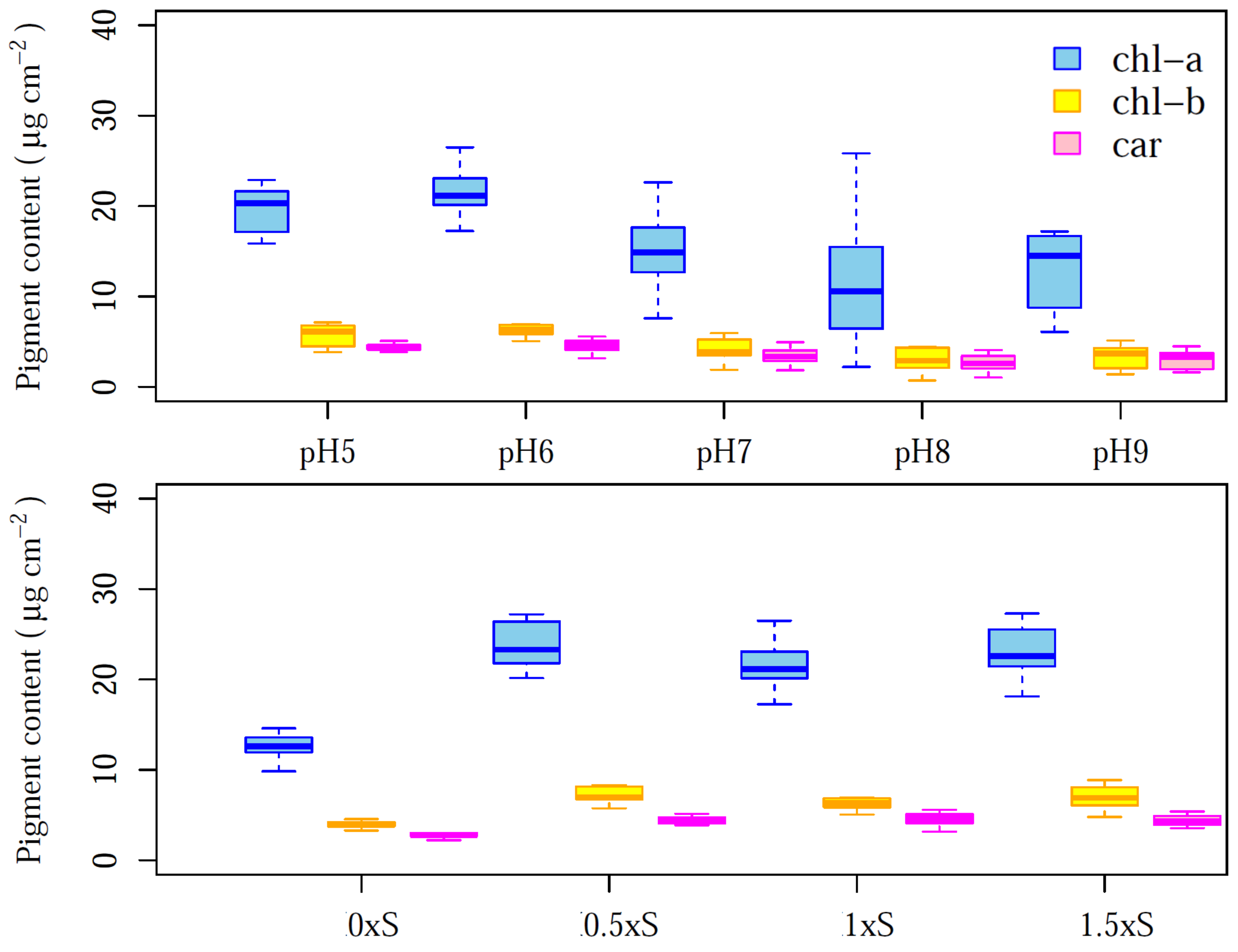
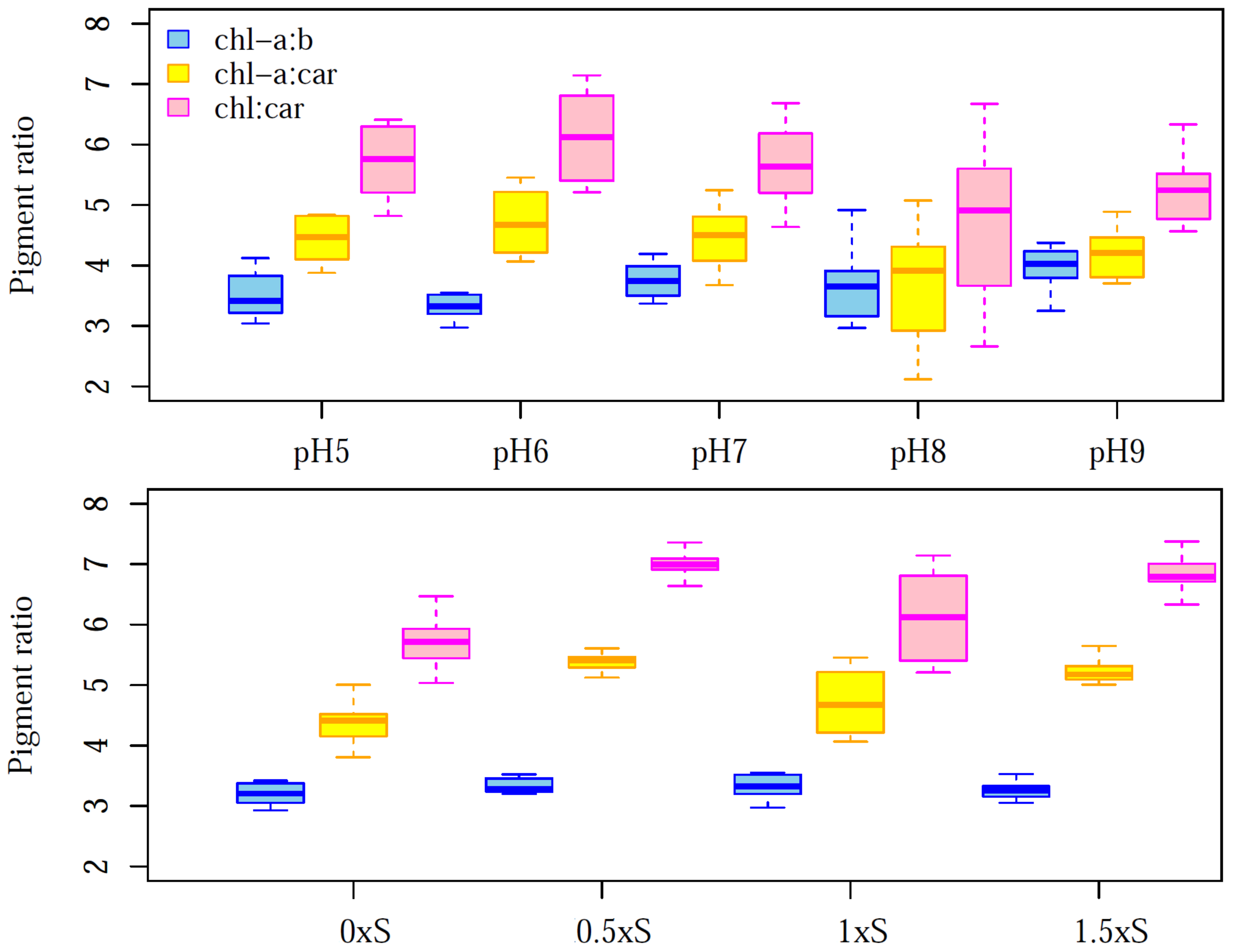
Figure 2 shows the boxplots of the chl a, b, and car contents of the different pH conditions or S-strength treatments. The contents per leaf area (cm2) ranged from 9.84 to 27.29 μg for chl a, 2.91 to 8.91 μg for chl b, and 2.23 to 5.57 μg for car. There were no significant differences in photosynthetic pigments contents between the two cultivars among different pH conditions and S-strengths (p < 0.05, based on the Tukey–Kramer test). The relationships between the pigment ratios and pH conditions or S-strengths are shown in Figure 3. Their ranges were 2.93–4.92, 2.11–5.74, and 2.66–7.48 for chl a:b, chl a:car, and chl:car, respectively. For the chl a:b ratio, significant differences were not confirmed between the two cultivars nor among S-strength treatments, while significant differences were confirmed between two cultivars for pH 5; pH 5 and 9 for Mazuma; and pH 6 and 9 for Onimidori (p < 0.05, based on the Tukey–Kramer test).
Negative correlations were confirmed between the pH value and chl a, b and car. The correlations of Mazuma were stronger than those of Onimidori (Table 1). Although a negative correlation was also confirmed for chl a:car and chl:car, the correlation between pH and chl a:car was not significant when the dataset was separated by cultivars (p values were 0.206 and 0.054 for Onimidori and Mazuma, respectively). On the contrary, a positive correlation was confirmed between pH and chl a:b; it was significant for all, as well as for Mazuma. The photosynthetic pigments contents and S-strength were more strongly correlated with the photosynthetic pigment contents than with pH. This positive correlation was generally confirmed, except for chl a, b of Mazuma (r = −0.328, p = 0.158).

3.2. Spectral Patterns

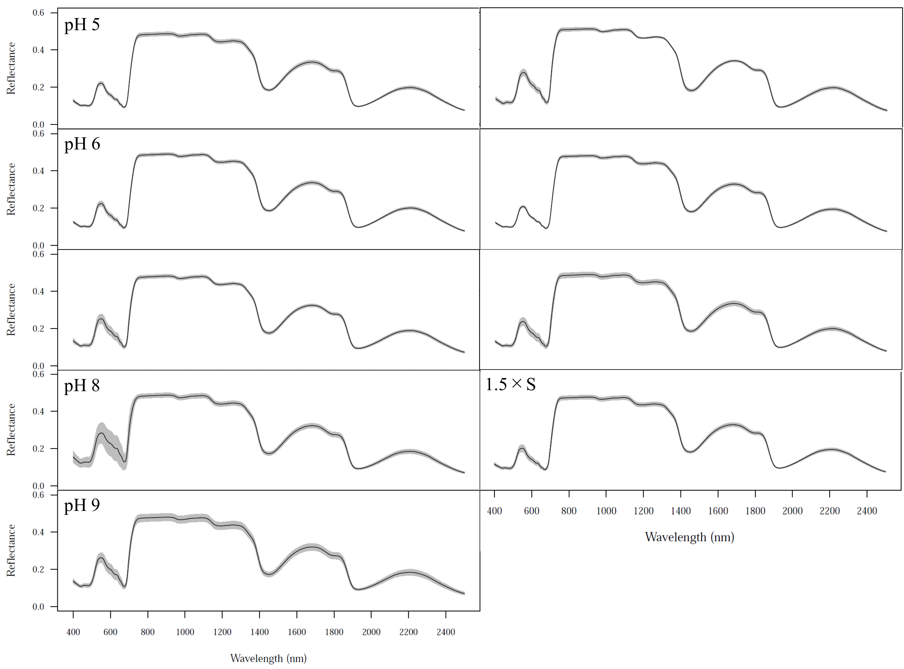
The mean reflectance spectra and standard deviations for each pH condition and S strength are shown in Figure 4. Generally, some differences in spectra were confirmed over the domain between 400 and 900 nm among the pH conditions or S-strength values. Table 2 and Table 3 show the effective wavelength to distinguish five pH conditions or four S-strengths based on the stepwise discriminant analysis (p < 0.001). To classify five different pH conditions, the ends of the red edge bands (706–756 nm) were effective. Then, they were selected for OR, FDR, DT, MSC, and SNV, while a green-peak band (536 nm) was selected for CR. For FDR, the start of the red edge bands (614 and 619 nm) was also selected. Reflectance values near 700 nm were also effective for identifying samples at four S-strengths; this domain was selected for all spectra. Additionally, a green peak band (514 nm) was selected for OR, and 893 nm was selected for CR.

3.3. Accuracy Assessment

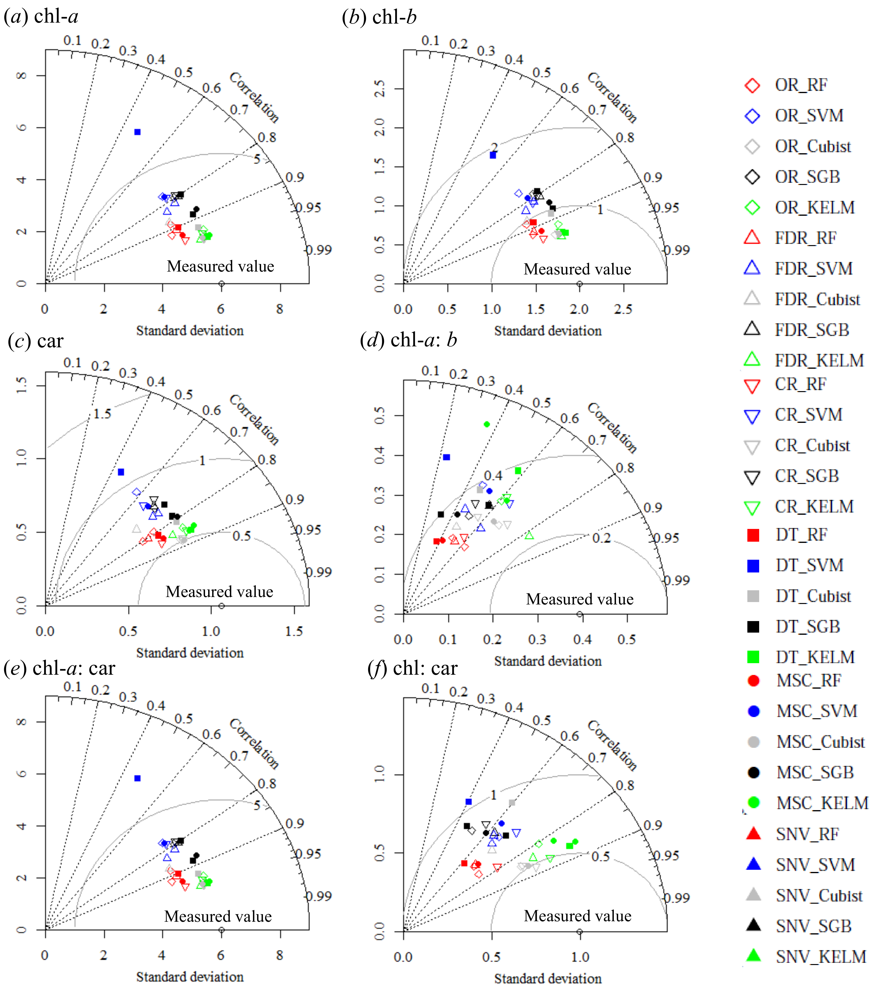
The performances of the regression models based on the machine learning algorithms are shown in Figure 5. Based on the mean RPD values of 100 repetitions, the best pre-processing and algorithm combinations were DT–KELM for chl a (RPD = 1.511–5.17, RMSE = 1.23–3.62 μg cm−2) and chl a:b (RPD = 0.73–3.17, RMSE = 0.13–0.60); CR–KELM for chl b (RPD = 1.92–5.06, RMSE = 0.41–1.03 μg cm−2) and chl a:car (RPD = 1.31–3.23, RMSE = 0.26–0.50); SNV–Cubist for car (RPD = 1.63–3.32, RMSE = 0.31–1.89 μg cm−2); and DT–Cubist for chl:car (RPD = 1.53–3.96, RMSE = 0.27–0.74). OR was acceptable for the chl a estimation when RF or KELM was applied to generate the regression models. Then, OR–RF, OR–KELM, FDR–RF, FDR–KELM, CR–RF, CR–KELM, DT–RF, DT–Cubist, DT–KELM, MSC–KELM, SNV–RF, SNV–Cubist, and SVN–KELM always had RPD values more than 1.4. For the chl b estimation, RF was also applicable to OR, and OR–RF, FDR–RF, FDR–KELM, CR–RF, CR–KELM, DT–RF, DT–Cubist, DT–KELM, MSC–KELM, SNV–RF, SNV–Cubist, and SNV–KELM were always categorized as “A” or “B”. Poor models, namely those in “Category C”, were confirmed in some cases when OR was used for estimating car.
To estimate the ratio of chl a:b, chl a:car, and total chl:car, there were not always applicable combinations of pre-processing and machine learning algorithms except for the total chl:car estimation based on DT–Cubist. Nevertheless, Cubist and KELM possessed mean RPD vales with all the pre-processing for chl a:car and total chl:car. Although KELM still possessed the mean RPD values greater than 1.4 for chl a:b, except for SNV, the RMSE of SNV–KELM was greater than and the averaged RPD values were less than for the combinations with SNV (mean RPD value of 1.24).
Table 4 and Table 5 show the optimal combinations of pre-processing techniques and machine learning algorithms and the differences in RPD values between the directed estimations of their ratios. The best combinations were DT–KELM for chl a, FDR–KELM for chl b and chl a:b, DT–Cubist for car and chl:car, and CR-KELM for chl a:car.

3.4. Sensitivity Analysis

The importance of each wavelength was evaluated based on the DSA for each algorithm at a 25-nm interval. Generally, RF, Cubist, and SGB had double peaks at 550–575 and 700–725 nm for all the spectra. Although this tendency was also confirmed for SVM and KELM, their importance was relatively lower than RF, Cubist, and SGB; the peaks were obscure. For MSC and SNV, small peaks were confirmed for RF and SNV. For RF, the green peak had a greater influence on chl b estimations than on chl b estimations for all spectra; this tendency was obscure for the other algorithm. The importance at 400–425 nm of SGM was also high for OR, DT, MSC, and SNV. Similar to the chl a estimation, the two peaks for all the spectra and the importance at 400–425 nm of SGM were confirmed. However, the importance near 650–675 nm of FDR was higher than that of chl a. For the car estimation, the high importance near 530 nm was confirmed from OR, FDR, CR, and MSC. However, the two peaks were also confirmed from FDR, MSC, and SNV near 1875–1900 and 2000–2025 nm for RF, Cubist, and SGB.
The importance values for chl a:b were relatively low, and no band possessed an importance more than 10% except for the combinations of Cubist and DT or FDB. However, peaks at 675–700 nm were confirmed for OR, FDR, DT, and SNV, a peak near 1150–1175 nm for MSC, a peak at 1375–1400 nm for OR and DT, and a peak at 1425–1450 nm for FDR. The patterns of importance distribution were similar between the chl a:car and chl:car estimations. The high importance at 400–425 nm of SGB was also confirmed for OR, DT, MSC, and SNV. While the peak near 700–725 nm was confirmed for OR, FDR, CR, and DT, OR also possessed a peak near 625–650 nm. MSC possessed a peak near 2075–2100 nm.

4. Discussion

4.1. Characteristics of the Samples Used in This Study

Changing chl a:b is either caused by the kind of materials involved or by the different developmental stages, fertilizers, chemicals, moisture, and other environments. Chl a:b is considered generally to be 3 [85] and is positively correlated with the ratio of the PSII cores to the light-harvesting chlorophyll–protein complex [86]. In this study, the mean chl a:b values were 3.21, 3.33, 3.33, and 3.29 for samples under pH 5–9; and 3.52, 3.33, 3.75, 3.68, and 3.95 for samples under 0×S, 0.5×S, 1×S, and 1.5×S. These values were larger than 3, representative of causing stress under high-light or nitrogen-lacking conditions. Furthermore, chl:car is also a good indicator for evaluating environmental stress in plants [8]. There was a linear relationship between the formation of light-harvesting complex II (LHCII) aggregates and nonphotochemical quenching [87]. The increase in chl:car implies an increase in LHCII [88]. The mean chl:car values were 5.73, 6.11, 5.64, 4.76, and 5.31 for samples under pH 5–9 and 5.68, 7.02, 6.11, and 6.83 for samples under 0×S, 0.5×S, 1×S, and 1.5×S, respectively. Chl a:car possessed a significant positive correlation with chl:car in this study (r = 0.99, p < 0.001) and has been used to evaluate light stress and Light-Harvesting Complex Stress [9,89]. The mean chl a:car values were 4.47, 4.69, 4.44, 3.71, and 4.23 for samples under pH 5–9 and 4.33, 5.40, 4.69, and 5.24 for samples under 0×S, 0.5×S, 1×S, and 1.5×S, respectively. The values of some datasets published online are 2.99 in the LOPEX dataset and 3.45 in the HAWAII dataset [9]. These indicators imply that the dataset used in this study included measurements under high-stress environments.

4.2. Performance of Different Pre-Processing and Machine Learning Algorithms

DT was the best or second-best technique, and its combinations with KELM or Cubist were effective for all the parameters focused on in this study. The advantages of SNV were not fully confirmed, although it was the second-best technique for estimating chl:car. DT shows an excellent performance in removing the effects of baseline shift and curvilinearity from the original reflectance [50]; it was also effective in improving accuracies. MSC and SNV were also adjusted for baseline shifts between samples, and more corrections could be conducted than with DT. For instance, MSC minimizes the additive and multiplicative effects in reflectance, and SNV removes the multiplicative interferences of scatter and particle size [90]. However, leaf-scale measurements were conducted with leaf-clips in this study, and more corrections may not be required. As a result, their advantages have not been shown in this study, and slop corrections were not required for the study data. As a result, FDR, which is effective in enhancing resolution, as well as correcting baseline shifts [91], but is influenced by slop errors, also showed high performances for chl a, b and their ratios. CR was effective in estimating the car-related parameters (i.e., car, chl a:car, and chl:car). In this study, reflectance values at 400 nm and the end of the red edge were normally selected as the continuum endpoints, enhancing the changes near the green peaks. Many studies have shown the advantage of green peaks for estimating car and some vegetation indices based on green peaks have been previously proposed [92,93,94,95,96]. CR also succeeded in enhancing the green peak features.
Generally, KELM and Cubist were the best algorithms. KELM possessed better performances for estimating chl a, b and their ratios, while Cubist was more effective in estimating car. SVM and KELM are kernel-based algorithms and, thus, an inappropriate selection of hyperparameters related to kernel function made the estimation accuracies worse [97]. A grid search was used to find an adequate set of hyperparameters of SVM in previous studies, with several suitable combinations being found for the training data [98,99]. However, some of the combinations are not applicable to other datasets as they result in overfitting. This phenomenon was also confirmed in this study, in which the Bayesian optimization was applied to tune the hyperparameters, confirming the RPD values less than 1.0 (for example, 11 times for chl a estimations based on OR). In contrast, the variances of Kp were smaller than σ. RF, Cubist, and SGB are stochastic modelling techniques involving ensemble regression trees or rule-based models; the high performances of Cubist and SGB have been reported in previous studies [42]. Although the high performance of Cubist was also confirmed in this study, the accuracies of SGB were the worst at 12, 19, 18, 22, 43, and 37 times for chl a, b, car, chl a:car, and chl:car, respectively. SGB improves the robustness for imbalanced training data dealing with interactions and avoids problems arising from a wrong learning rate [76]. However, sampling a fraction of the training data was required in this strategy. The sample size might be too small to obtain fractions from the training data, leading to overfitting. The better performance of Cubist compared to RF was reported in previous studies [42,100,101] and confirmed in this study.
The differences in reflectance between healthy and stressed vegetation can be detected in changes to the green peak and the red edge [102], and then the shifts of the green peak and the red edge inflexion point were confirmed within the pH conditions or S strengths (Figure 4). For estimating the photosynthetic pigment contents, the importance at the green peak and the red edge inflexion point was larger when RF was applied; on the contrary, their importance was obscure for KELM. In order to avoid these phenomena, KELM could be a better option.

4.3. Direct Estimation vs. Indirect Estimation for Pigment Ratio

In this study, the regression models were generated directly to estimate the pigment ratio. However, these ratios could be calculated from the estimation results of chl a, b and car. Therefore, the estimation accuracies were compared to more accurate stress evaluations. For the RPD values from the estimated chl a, b and car, the direct estimations were generally superior to the indirect estimations. Therefore, direct estimations should be used to evaluate the stress of plants. Although the differences of CR–RF, MSC–RF, and MSC–Cubist for chl:car were significantly negative values (p < 0.01 based on a t-test), their RPD values were still poor compared with other combinations between the pre-processing and machine learning algorithms. As such, CR–RF, MSC–RF, and MSC–Cubist could not be a better choice for estimating chl:car.
It was reported that chl:car estimation based on hyperspectral reflectance is not straightforward due to non-obvious absorption features in the visible spectral range [103]. In this study, this phenomenon was also confirmed for chl a:b and chl a:car, and the advantages of direct estimation were clearer for them, which implied hyperspectral reflectance could detect some physiological signal and could be widely used in stress detection. As a result, the reflectance values at some wavelengths allowed for evaluating the risk of early mortality as well as the appearance and ingredients of wasabi before their cultivation.

5. Conclusions

The potential of vegetation reflectance for quantifying three photosynthetic pigment contents, including chlorophyll a, b and carotenoid, and their ratios, was evaluated for wasabi. In this study, five pre-processing techniques, first derivative reflectance (FDR), continuum-removal (CR) transformation, de-trending (DT), multiplicative scatter correction (MSC), and standard normal variate (SNV), were applied in addition to the original reflectance using five machine learning algorithms (random forests (RF), support vector machine (SVM), kernel-based extreme learning machine (KELM), Cubist, and Stochastic Gradient Boosting (SGB)). The superior usefulness of CR, DT, and SVN was confirmed, and the combination with KELM or Cubist was most effective for estimating the content of the three photosynthetic pigments and their ratios. For carotenoid estimation, OR was selected 22 times as having the best hyperspectral data, and it was still useful. However, the spectrum after pre-processing was selected more than 80 times for estimating leaf chlorophyll a, b contents and pigment ratios. This implied that pre-processing helps improve the estimation accuracies and can be used for the in situ measurements of leaf properties.
According to the results, hyperspectral data allowed for evaluating the stresses as well as the appearance and ingredients of wasabi before their cultivation, and the information provided from hyperspectral reflectance can be used to carry out more suitable nutrient management, facilitating quality control and plant maintenance for less experienced farmers.

Supplementary Materials

The following are available online at https://www.mdpi.com/2072-4292/12/19/3265/s1, Table S1: Mean reflectance spectra and standard deviations for the different pH conditions or S-strength treatments, Table S2: Estimated values from OR, Table S3: Estimated values from FDR, Table S4: Estimated values from CR, Table S5: Estimated values from DT, Table S6: Estimated values from MSC, Table S7: Estimated values from SNV.

Author Contributions

H.Y., H.M., T.I., and A.M. designed the wasabi cultivation system; R.S. measured the hyperspectral reflectance; H.Y. and H.M. measured the pigment contents; R.S. analysed the data and wrote the manuscript. All authors have read and agreed to the published version of the manuscript.

Funding

This study was supported financially by the Kurita Water and Environment Foundation (KWEF, Japan) research grant award (ID: 19B001), the Yamazaki Spice Promotion Foundation, and JSPS KAKENHI (grant number 19K06313).

Conflicts of Interest

The author declares no conflict of interest.

References

  1. Gitelson, A.A.; Vina, A.; Verma, S.B.; Rundquist, D.C.; Arkebauer, T.J.; Keydan, G.; Leavitt, B.; Ciganda, V.; Burba, G.G.; Suyker, A.E. Relationship between gross primary production and chlorophyll content in crops: Implications for the synoptic monitoring of vegetation productivity. J. Geophys. Res. Atmos. 2006, 111. [Google Scholar] [CrossRef] [Green Version]
  2. Leong, T.Y.; Anderson, J.M. Adaptation of the thylakoid membranes of pea chloroplasts to light intensities. I. Study on the distribution of chlorophyll-protein complexes. Photosynth. Res. 1984, 5, 105–115. [Google Scholar] [CrossRef] [PubMed]
  3. Chen, W.M.; Jin, N.; Shi, Y.; Su, Y.Q.; Fei, B.J.; Li, W.; Qiao, D.R.; Cao, Y. Coordinate expression of light-harvesting chlorophyll a/b gene family of photosystem II and chlorophyll a oxygenase gene regulated by salt-induced phosphorylation in Dunaliella salina. Photosynthetica 2010, 48, 355–360. [Google Scholar] [CrossRef]
  4. Hobe, S.; Fey, H.; Rogl, H.; Paulsen, H. Determination of relative chlorophyll binding affinities in the major light-harvesting chlorophyll a/b complex. J. Biol. Chem. 2003, 278, 5912–5919. [Google Scholar] [CrossRef] [Green Version]
  5. Datt, B. Visible/near infrared reflectance and chlorophyll content in Eucalyptus leaves. Int. J. Remote Sens. 1999, 20, 2741–2759. [Google Scholar] [CrossRef]
  6. Demmig Adams, B.; Gilmore, A.M.; Adams, W.W. Carotenoids. In vivo functions of carotenoids in higher plants. Faseb. J. 1996, 10, 403–412. [Google Scholar] [CrossRef]
  7. Edge, R.; McGarvey, D.J.; Truscott, T.G. The carotenoids as anti-oxidants—A review. J. Photochem. Photobiol. B Biol. 1997, 41, 189–200. [Google Scholar] [CrossRef]
  8. Hendry, G.A.F.; Price, A.H. Stress Indicators: Chlorophylls and Carotenoids; Chapman Hall: London, UK, 1993. [Google Scholar]
  9. Féret, J.-B.; Francois, C.; Asner, G.P.; Gitelson, A.A.; Martin, R.E.; Bidel, L.P.R.; Ustin, S.L.; le Maire, G.; Jacquemoud, S. PROSPECT-4 and 5: Advances in the leaf optical properties model separating photosynthetic pigments. Remote Sens. Environ. 2008, 112, 3030–3043. [Google Scholar] [CrossRef]
  10. Sonobe, R.; Hirono, Y.; Oi, A. Non-Destructive Detection of Tea Leaf Chlorophyll Content Using Hyperspectral Reflectance and Machine Learning Algorithms. Plants 2020, 9, 368. [Google Scholar] [CrossRef] [Green Version]
  11. Sonobe, R.; Hirono, Y.; Oi, A. Quantifying chlorophyll-a and b content in tea leaves using hyperspectral reflectance and deep learning. Remote Sens. Lett. 2020, 11, 933–942. [Google Scholar] [CrossRef]
  12. Sonobe, R.; Yamashita, H.; Mihara, H.; Morita, A.; Ikka, T. Hyperspectral reflectance sensing for quantifying leaf chlorophyll content in wasabi leaves using spectral pre-processing techniques and machine learning algorithms. Int. J. Remote Sens. 2020. [Google Scholar] [CrossRef]
  13. Sonobe, R.; Miura, Y.; Sano, T.; Horie, H. Monitoring Photosynthetic Pigments of Shade-Grown Tea from Hyperspectral Reflectance. Can. J. Remote Sens. 2018, 44, 104–112. [Google Scholar] [CrossRef]
  14. Hege, N.; Kobayashi, M.; Michiki, N.; Takano, T.; Baba, F.; Kobayashi, K.; Ohyanagi, H.; Ohgane, J.; Yano, K.; Yamane, K. Complete chloroplast genome sequence and phylogenetic analysis of wasabi (Eutrema japonicum) and its relatives. Sci. Rep. 2019, 9, 14377. [Google Scholar]
  15. Li, S.J.; Gao, L.H.; Zhou, S.P.; Liu, G.Q.; Liu, W. Diversification of vegetable growing in the middle and lower reaches of the Yangtze River. Third Int. Symp. Diversif. Veg. Crop. 1998, 467, 253–258. [Google Scholar]
  16. Prado-Cabrero, A.; Beatty, S.; Howard, A.; Stack, J.; Bettin, P.; Nolan, J.M. Assessment of lutein, zeaxanthin and meso-zeaxanthin concentrations in dietary supplements by chiral high-performance liquid chromatography. Eur. Food Res. Technol. 2016, 242, 599–608. [Google Scholar] [CrossRef] [Green Version]
  17. Bilger, W.; Bjorkman, O.; Thayer, S.S. Light-induced spectral absorbance changes in relation to photosynthesis and the epoxidation state of xanthophyll cycle components in cotton leaves. Plant Physiol. 1989, 91, 542–551. [Google Scholar] [CrossRef]
  18. Yang, X.; Tang, J.W.; Mustard, J.F.; Wu, J.; Zhao, K.G.; Serbin, S.; Lee, J.E. Seasonal variability of multiple leaf traits captured by leaf spectroscopy at two temperate deciduous forests. Remote Sens. Environ. 2016, 179, 1–12. [Google Scholar] [CrossRef] [Green Version]
  19. Jacquemoud, S.É.P.; Ustin, S. Leaf Optical Properties; Cambridge University Press: Cambridge, UK, 2019. [Google Scholar]
  20. Yamamoto, A.; Nakamura, T.; Adu-Gyamfi, J.J.; Saigusa, M. Relationship between chlorophyll content in leaves of sorghum and pigeonpea determined by extraction method and by chlorophyll meter (SPAD-502). J. Plant Nutr. 2002, 25, 2295–2301. [Google Scholar] [CrossRef]
  21. Sonobe, R.; Wang, Q. Towards a Universal Hyperspectral Index to Assess Chlorophyll Content in Deciduous Forests. Remote Sens. 2017, 9, 191. [Google Scholar] [CrossRef] [Green Version]
  22. Lu, B.; He, Y.H. Evaluating Empirical Regression, Machine Learning, and Radiative Transfer Modelling for Estimating Vegetation Chlorophyll Content Using Bi-Seasonal Hyperspectral Images. Remote Sens. 2019, 11, 1979. [Google Scholar] [CrossRef] [Green Version]
  23. Shah, S.H.; Angel, Y.; Houborg, R.; Ali, S.; McCabe, M.F. A Random Forest Machine Learning Approach for the Retrieval of Leaf Chlorophyll Content in Wheat. Remote Sens. 2019, 11, 920. [Google Scholar] [CrossRef] [Green Version]
  24. Vanbrabant, Y.; Tits, L.; Delalieux, S.; Pauly, K.; Verjans, W.; Somers, B. Multitemporal Chlorophyll Mapping in Pome Fruit Orchards from Remotely Piloted Aircraft Systems. Remote Sens. 2019, 11, 1468. [Google Scholar] [CrossRef] [Green Version]
  25. Sonobe, R.; Wang, Q. Assessing the xanthophyll cycle in natural beech leaves with hyperspectral reflectance. Funct. Plant Biol. 2016, 43, 438–447. [Google Scholar] [CrossRef] [PubMed]
  26. Gamon, J.A.; Penuelas, J.; Field, C.B. A narrow-waveband spectral index that tracks diurnal changes in photosynthetic efficiency. Remote Sens. Environ. 1992, 41, 35–44. [Google Scholar] [CrossRef]
  27. Gamon, J.A.; Field, C.B.; Bilger, W.; Bjorkman, O.; Fredeen, A.L.; Penuelas, J. Remote sensing of the xanthophyll cycle and chlorophyll fluorescence in sunflower leaves and canopies. Oecologia 1990, 85, 1–7. [Google Scholar] [CrossRef] [PubMed]
  28. Skoneczny, H.; Kubiak, K.; Spiralski, M.; Kotlarz, J. Fire Blight Disease Detection for Apple Trees: Hyperspectral Analysis of Healthy, Infected and Dry Leaves. Remote Sens. 2020, 12, 2101. [Google Scholar] [CrossRef]
  29. Li, Z.H.; Jin, X.L.; Wang, J.H.; Yang, G.J.; Nie, C.W.; Xu, X.G.; Feng, H.K. Estimating winter wheat (Triticum aestivum) LAI and leaf chlorophyll content from canopy reflectance data by integrating agronomic prior knowledge with the PROSAIL model. Int. J. Remote Sens. 2015, 36, 2634–2653. [Google Scholar] [CrossRef]
  30. Masemola, C.; Cho, M.A.; Ramoelo, A. Comparison of Landsat 8 OLI and Landsat 7 ETM + for estimating grassland LAI using model inversion and spectral indices: Case study of Mpumalanga, South Africa. Int. J. Remote Sens. 2016, 37, 4401–4419. [Google Scholar] [CrossRef]
  31. Izzuddin, M.A.; Idris, A.S.; Nisfariza, M.N.; Nordiana, A.A.; Shafri, H.Z.M.; Ezzati, B. The development of spectral indices for early detection of Ganoderma disease in oil palm seedlings. Int. J. Remote Sens. 2017, 38, 6505–6527. [Google Scholar] [CrossRef]
  32. Jacquemoud, S.; Baret, F. PROSPECT: A Model of leaf optical properties spectra. Remote Sens. Environ. 1990, 34, 75–91. [Google Scholar] [CrossRef]
  33. Féret, J.-B.; Gitelson, A.A.; Noble, S.D.; Jacquemoud, S. PROSPECT-D: Towards modeling leaf optical properties through a complete lifecycle. Remote Sens. Environ. 2017, 193, 204–215. [Google Scholar] [CrossRef] [Green Version]
  34. Hosgood, B.; Jacquemoud, S.; Andreoli, G.; Verdebout, J.; Pedrini, G.; Schmuck, G. Leaf Optical Properties EXperiment 93; Office for Official Publications of the European Communities: Luxembourg, 1994; p. 20. [Google Scholar]
  35. Sonobe, R.; Wang, Q. Hyperspectral indices for quantifying leaf chlorophyll concentrations performed differently with different leaf types in deciduous forests. Ecol. Inform. 2017, 37, 1–9. [Google Scholar] [CrossRef]
  36. Doktor, D.; Lausch, A.; Spengler, D.; Thurner, M. Extraction of Plant Physiological Status from Hyperspectral Signatures Using Machine Learning Methods. Remote Sens. 2014, 6, 12247–12274. [Google Scholar] [CrossRef] [Green Version]
  37. Biau, G.; Scornet, E. A random forest guided tour. Test 2016, 25, 197–227. [Google Scholar] [CrossRef] [Green Version]
  38. Oliveira, R.A.; Nasi, R.; Niemelainen, O.; Nyholm, L.; Alhonoja, K.; Kaivosoja, J.; Jauhiainen, L.; Viljanen, N.; Nezami, S.; Markelin, L.; et al. Machine learning estimators for the quantity and quality of grass swards used for silage production using drone-based imaging spectrometry and photogrammetry. Remote Sens. Environ. 2020, 246, 20. [Google Scholar] [CrossRef]
  39. Burges, C.J.C. A tutorial on Support Vector Machines for pattern recognition. Data Min. Knowl. Discov. 1998, 2, 121–167. [Google Scholar] [CrossRef]
  40. Houborg, R.; McCabe, M.F. A hybrid training approach for leaf area index estimation via Cubist and random forests machine-learning. Isprs. J. Photogramm. Remote Sens. 2018, 135, 173–188. [Google Scholar] [CrossRef]
  41. Wijesingha, J.; Astor, T.; Schulze-Bruninghoff, D.; Wengert, M.; Wachendorf, M. Predicting Forage Quality of Grasslands Using UAV-Borne Imaging Spectroscopy. Remote Sens. 2020, 12, 126. [Google Scholar] [CrossRef] [Green Version]
  42. Breunig, F.M.; Galvao, L.S.; Dalagnol, R.; Dauve, C.E.; Parraga, A.; Santi, A.L.; Della Flora, D.P.; Chen, S.S. Delineation of management zones in agricultural fields using cover crop biomass estimates from PlanetScope data. Int. J. Appl. Earth Obs. Geoinf. 2020, 85. [Google Scholar] [CrossRef]
  43. Maliha, A.; Yusof, R.; Shapiai, M.I. Extreme learning machine for structured output spaces. Neural Comput. Appl. 2018, 30, 1251–1264. [Google Scholar] [CrossRef]
  44. Sonobe, R.; Sano, T.; Horie, H. Using spectral reflectance to estimate leaf chlorophyll content of tea with shading treatments. Biosyst. Eng. 2018, 175, 168–182. [Google Scholar] [CrossRef]
  45. Meng, X.T.; Bao, Y.L.; Liu, J.G.; Liu, H.J.; Zhang, X.L.; Zhang, Y.; Wang, P.; Tang, H.T.; Kong, F.C. Regional soil organic carbon prediction model based on a discrete wavelet analysis of hyperspectral satellite data. Int. J. Appl. Earth Obs. Geoinf. 2020, 89. [Google Scholar] [CrossRef]
  46. Inoue, Y.; Sakaiya, E.; Zhu, Y.; Takahashi, W. Diagnostic mapping of canopy nitrogen content in rice based on hyperspectral measurements. Remote Sens. Environ. 2012, 126, 210–221. [Google Scholar] [CrossRef]
  47. Roman, J.R.; Rodriguez-Caballero, E.; Rodriguez-Lozano, B.; Roncero-Ramos, B.; Chamizo, S.; Aguila-Carricondo, P.; Canton, Y. Spectral Response Analysis: An Indirect and Non-Destructive Methodology for the Chlorophyll Quantification of Biocrusts. Remote Sens. 2019, 11, 1350. [Google Scholar] [CrossRef] [Green Version]
  48. Miller, D.L.; Alonzo, M.; Roberts, D.A.; Tague, C.L.; McFadden, J.P. Drought response of urban trees and turfgrass using airborne imaging spectroscopy. Remote Sens. Environ. 2020, 240. [Google Scholar] [CrossRef]
  49. Liang, K.; Huang, J.N.; He, R.Y.; Wang, Q.J.; Chai, Y.Y.; Shen, M.X. Comparison of Vis-NIR and SWIR hyperspectral imaging for the non-destructive detection of DON levels in Fusarium head blight wheat kernels and wheat flour. Infrared Phys. Technol. 2020, 106, 9. [Google Scholar] [CrossRef]
  50. Barnes, R.J.; Dhanoa, M.S.; Lister, S.J. Standard normal variate transformation and de-trending of near-infrared diffuse reflectance spectra. Appl. Spectrosc. 1989, 43, 772–777. [Google Scholar] [CrossRef]
  51. Hoagland, D.R.; Arnon, D.I. The water-culture method for growing plants without soil. Circular 1938, 347, 1884–1949. [Google Scholar]
  52. Sultana, T.; Savage, G.P.; McNeil, D.L.; Porter, N.G.; Martin, R.J.; Deo, B. Effects of fertilisation on the allyl isothiocyanate profile of above-ground tissues of New Zealand-grown wasabi. J. Sci. Food Agric. 2002, 82, 1477–1482. [Google Scholar] [CrossRef]
  53. Prasad, K.A.; Gnanappazham, L.; Selvam, V.; Ramasubramanian, R.; Kar, C.S. Developing a spectral library of mangrove species of Indian east coast using field spectroscopy. Geocarto Int. 2015, 30, 580–599. [Google Scholar] [CrossRef]
  54. Wellburn, A.R. The spectral determination of chlorophyll a and chlorophyll b, as well as total carotenoids, using various solvents with spectrophotometers of different resolution. J. Plant Physiol. 1994, 144, 307–313. [Google Scholar] [CrossRef]
  55. Hastie, T.; Tibshirani, R.; Friedman, J. The Elements of Statistical Learning: Data Mining, Inference, and Prediction, 2nd ed.; Springer: New York, NY, USA, 2009; p. 745. [Google Scholar]
  56. Nguyen, K.A.; Chen, W.; Lin, B.S.; Seeboonruang, U.; Thomas, K. Predicting Sheet and Rill Erosion of Shihmen Reservoir Watershed in Taiwan Using Machine Learning. Sustainability 2019, 11, 3615. [Google Scholar] [CrossRef] [Green Version]
  57. Yan, L.; Pang, L.; Wang, H.; Xiao, J. Recognition of different Longjing fresh tea varieties using hyperspectral imaging technology and chemometrics. J. Food Process Eng. 2020, 43, 9. [Google Scholar] [CrossRef]
  58. Gopinath, G.; Sasidharan, N.; Surendran, U. Landuse classification of hyperspectral data by spectral angle mapper and support vector machine in humid tropical region of India. Earth Sci. Inform. 2020, 13, 633–640. [Google Scholar] [CrossRef]
  59. Sun, X.; Subedi, P.; Walker, R.; Walsh, K.B. NIRS prediction of dry matter content of single olive fruit with consideration of variable sorting for normalisation pre-treatment. Postharvest Biol. Technol. 2020, 163, 10. [Google Scholar] [CrossRef]
  60. Tsai, F.; Philpot, W. Derivative analysis of hyperspectral data. Remote Sens. Environ. 1998, 66, 41–51. [Google Scholar] [CrossRef]
  61. Clark, R.N.; Roush, T.L. Reflectance spectroscopy: Quantitative analysis techniques for remote sensing applications. J. Geophys. Res. Solid Earth 1984, 89, 6329–6340. [Google Scholar] [CrossRef]
  62. Ren, G.X.; Sun, Y.M.; Li, M.H.; Ning, J.M.; Zhang, Z.Z. Cognitive spectroscopy for evaluating Chinese black tea grades (Camellia sinensis): Near-infrared spectroscopy and evolutionary algorithms. J. Sci. Food Agric. 2020, 100, 3950–3959. [Google Scholar] [CrossRef]
  63. R Core Team. R: A language and Environment for Statistical Computing. R Foundation for Statistical Computing. Available online: https://www.R-project.org/ (accessed on 11 August 2020).
  64. Stevens, A.; Ramirez-Lopez, L. Package ‘prospectr’. Available online: https://cran.r-project.org/web/packages/prospectr/prospectr.pdf (accessed on 11 August 2020).
  65. Snoek, J.; Rippel, O.; Swersky, K.; Kiros, R.; Satish, N.; Sundaram, N.; Patwary, M.M.A.; Prabhat; Adams, R.P. Scalable Bayesian optimization using deep neural networks . In Proceedings of the 32nd International Conference on Machine Learning (ICML), Paris, Lille, 6–11 July 2015; pp. 2171–2180. [Google Scholar]
  66. Yan, Y. Bayesian Optimization of Hyperparameters. Available online: https://cran.r-project.org/web/packages/rBayesianOptimization/rBayesianOptimization.pdf (accessed on 11 August 2020).
  67. Breiman, L. Random forests. Mach. Learn. 2001, 45, 5–32. [Google Scholar] [CrossRef] [Green Version]
  68. Belgiu, M.; Csillik, O. Sentinel-2 cropland mapping using pixel-based and object-based time-weighted dynamic time warping analysis. Remote Sens. Environ. 2018, 204, 509–523. [Google Scholar] [CrossRef]
  69. Ishwaran, H. The effect of splitting on random forests. Mach. Learn. 2015, 99, 75–118. [Google Scholar] [CrossRef] [PubMed]
  70. Ishwaran, H.; Kogalur, U.B. Random survival forests for R. R News 2007, 7, 25–31. [Google Scholar]
  71. Ding, S.F.; Shi, Z.Z.; Tao, D.C.; An, B. Recent advances in Support Vector Machines. Neurocomputing 2016, 211, 1–3. [Google Scholar] [CrossRef]
  72. Meyer, D.; Dimitriadou, E.; Hornik, K.; Weingessel, A.; Leisch, F.; Chang, C.-C.; Lin, C.-C. Misc Functions of the Department of Statistics, Probability. Available online: https://rdrr.io/rforge/e1071/e1071.pdf (accessed on 7 September 2020).
  73. Huang, G.B.; Zhu, Q.-Y.; Siew, C.-K. Extreme Learning Machine: A New Learning Scheme of Feedforward Neural Networks. In Proceedings of the International Joint Conference on Neural Networks (IJCNN2004), Budapest, Hungary, 25–29 July 2004; pp. 985–990. [Google Scholar]
  74. Quinlan, J.R. Learning with Continuous Classe AI ’92 . In Proceedings of the 5th Australian Joint Conference on Artificial Intelligence, Hobart, TAS, Australia, 16–18 November 1992; pp. 343–348. [Google Scholar]
  75. Kuhn, M.; Weston, S.; Keefer, C.; Coulter, N.; Quinlan, R.; Rulequest Research Pty Ltd. Package ‘Cubist’. Available online: https://cran.r-project.org/web/packages/Cubist/Cubist.pdf (accessed on 11 August 2020).
  76. Friedman, J.H. Stochastic gradient boosting. Comput. Stat. Data Anal. 2002, 38, 367–378. [Google Scholar] [CrossRef]
  77. Greenwell, B.; Boehmke, B.; Cunningham, J.; Developers, G. Package ‘GBM’. Available online: https://cran.r-project.org/web/packages/gbm/gbm.pdf (accessed on 11 August 2020).
  78. Burns, R.P.; Burns, R. Business Research Methods and Statistics Using SPSS; SAGE Publications: New York, NY, USA, 2008. [Google Scholar]
  79. Draper, N.H. Applied Regression Analysis; Wiley Series in Probability and Statistics; Wiley-Interscience: Hoboken, NJ, USA, 1998. [Google Scholar]
  80. Williams, P. Variables affecting near-infraredreflectance spectroscopic analysis. In Near-Infrared Technology in the Agricultural and Food Industries; Williams, P., Norris, K., Eds.; American Association of Cereal Chemists Inc.: Saint Paul, MN, USA, 1987; pp. 143–167. [Google Scholar]
  81. Ishwaran, H. Variable importance in binary regression trees and forests. Electron. J. Stat. 2007, 1, 519–537. [Google Scholar] [CrossRef]
  82. Sonobe, R. Parcel-Based Crop Classification Using Multi-Temporal TerraSAR-X Dual Polarimetric Data. Remote Sens. 2019, 11, 1148. [Google Scholar] [CrossRef] [Green Version]
  83. Cortez, P.; Embrechts, M.J. Using sensitivity analysis and visualization techniques to open black box data mining models. Inf. Sci. 2013, 225, 1–17. [Google Scholar] [CrossRef] [Green Version]
  84. Kewley, R.H.; Embrechts, M.J.; Breneman, C. Data strip mining for the virtual design of pharmaceuticals with neural networks. IEEE Trans. Neural Netw. 2000, 11, 668–679. [Google Scholar] [CrossRef] [Green Version]
  85. Katayama, Y.; Shida, S. Studies on the Change of Chlorophyll a and b Contents Due to Projected Materials and Some Environmental Conditions. Cytologia 1970, 35, 171–180. [Google Scholar] [CrossRef] [Green Version]
  86. Terashima, I.; Hikosaka, K. Comparative ecophysiology of leaf and canopy photosynthesis. Plant Cell Environ. 1995, 18, 1111–1128. [Google Scholar] [CrossRef]
  87. Tang, Y.L.; Wen, X.G.; Lu, Q.T.; Yang, Z.P.; Cheng, Z.K.; Lu, C.M. Heat stress induces an aggregation of the light-harvesting complex of photosystem II in spinach plants. Plant Physiol. 2007, 143, 629–638. [Google Scholar] [CrossRef] [PubMed] [Green Version]
  88. Embry, J.L.; Nothnagel, E.A. Leaf senescence of postproduction poinsettias in low-light stress. J. Am. Soc. Hortic. Sci. 1994, 119, 1006–1013. [Google Scholar] [CrossRef] [Green Version]
  89. Pinnola, A. The rise and fall of Light-Harvesting Complex Stress-Related proteins as photoprotection agents during evolution. J. Exp. Bot. 2019, 70, 5527–5535. [Google Scholar] [CrossRef] [PubMed]
  90. Rinnan, A.; van den Berg, F.; Engelsen, S.B. Review of the most common pre-processing techniques for near-infrared spectra. TrAC Trends Anal. Chem. 2009, 28, 1201–1222. [Google Scholar] [CrossRef]
  91. Bruning, B.; Berger, B.; Lewis, M.; Liu, H.; Garnett, T. Approaches, applications, and future directions for hyperspectral vegetation studies: An emphasis on yield-limiting factors in wheat. Plant Phenome J. 2020, 3. [Google Scholar] [CrossRef]
  92. Chappelle, E.W.; Kim, M.S.; McMurtrey, J.E. Ratio analysis of reflectance spectra (RARS): An algorithm for the remote estimation of the concentrations of chlorophyll A, chlorophyll B, and carotenoids in soybean leaves. Remote Sens. Environ. 1992, 39, 239–247. [Google Scholar] [CrossRef]
  93. Datt, B. Remote sensing of chlorophyll a, chlorophyll b, chlorophyll a + b, and total carotenoid content in eucalyptus leaves. Remote Sens. Environ. 1998, 66, 111–121. [Google Scholar] [CrossRef]
  94. Gitelson, A.A.; Zur, Y.; Chivkunova, O.B.; Merzlyak, M.N. Assessing carotenoid content in plant leaves with reflectance spectroscopy. Photochem. Photobiol. 2002, 75, 272–281. [Google Scholar] [CrossRef]
  95. Hernandez-Clemente, R.; Navarro-Cerrillo, R.M.; Zarco-Tejada, P.J. Carotenoid content estimation in a heterogeneous conifer forest using narrow-band indices and PROSPECT plus DART simulations. Remote Sens. Environ. 2012, 127, 298–315. [Google Scholar] [CrossRef]
  96. Sonobe, R.; Wang, Q. Nondestructive assessments of carotenoids content of broadleaved plant species using hyperspectral indices. Comput. Electron. Agric. 2018, 145, 18–26. [Google Scholar] [CrossRef]
  97. Horvath, G. CMAC neural network as an SVM with B-spline kernel functions. Proceedings of 20th IEEE Instrumentation and Measurement Technology Conference, Vail, CO, USA, 20–22 May 2003; pp. 1108–1113. [Google Scholar]
  98. Phienthrakul, T.; Kijsirikul, B. Evolutionary strategies for hyperparameters of support vector machines based on multi-scale radial basis function kernels. Soft Comput. 2010, 14, 681–699. [Google Scholar] [CrossRef]
  99. Trisasongko, B.H. Mapping stand age of rubber plantation using ALOS-2 polarimetric SAR data. Eur. J. Remote Sens. 2017, 50, 64–76. [Google Scholar] [CrossRef] [Green Version]
  100. Zhou, J.; Li, E.M.; Wei, H.X.; Li, C.Q.; Qiao, Q.Q.; Armaghani, D.J. Random Forests and Cubist Algorithms for Predicting Shear Strengths of Rockfill Materials. Appl. Sci. 2019, 9, 1621. [Google Scholar] [CrossRef] [Green Version]
  101. Walton, J.T. Subpixel urban land cover estimation: Comparing Cubist, Random Forests, and support vector regression. Photogramm. Eng. Remote Sens. 2008, 74, 1213–1222. [Google Scholar] [CrossRef] [Green Version]
  102. Zarco-Tejada, P.J.; Miller, J.R.; Noland, T.L.; Mohammed, G.H.; Sampson, P.H. Scaling-up and model inversion methods with narrowband optical indices for chlorophyll content estimation in closed forest canopies with hyperspectral data. IEEE Trans. Geosci. Remote Sens. 2001, 39, 1491–1507. [Google Scholar] [CrossRef] [Green Version]
  103. Zhou, X.F.; Huang, W.J.; Zhang, J.C.; Kong, W.P.; Casa, R.; Huang, Y.B. A novel combined spectral index for estimating the ratio of carotenoid to chlorophyll content to monitor crop physiological and phenological status. Int. J. Appl. Earth Obs. Geoinf. 2019, 76, 128–142. [Google Scholar] [CrossRef]
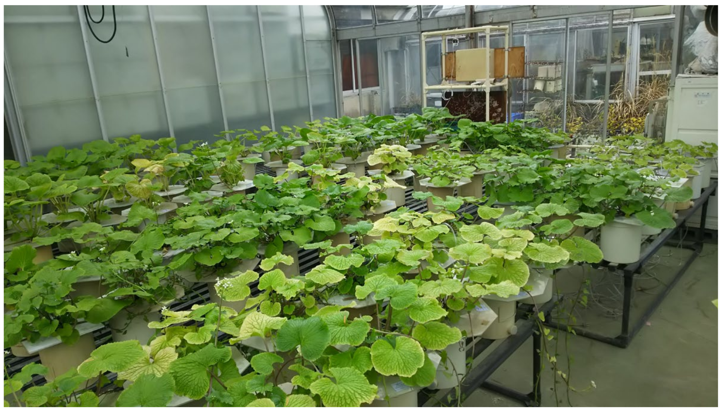
Figure 1. Hydroponic wasabi. Colours of some leaves changed due to stresses caused by pH conditions or S strengths.
Remotesensing 12 03265 g001
Figure 2. Boxplots of chl a, b and car for different pH conditions or sulphur ion concentrations (S strength). Although the highest contents were observed for the standard pH condition, 0.5×S was effective for the increase in photosynthetic pigment contents.
Remotesensing 12 03265 g002
Figure 3. Boxplots of pigment ratios for different pH conditions or S-strength treatments. A negative correlation was confirmed for chl a:car and chl:car with pH. On the contrary, a positive correlation was confirmed between pH and chl a:b.
Remotesensing 12 03265 g003
Figure 4. Mean reflectance spectra (solid lines) and standard deviations (thinner zones) for the different pH conditions or S-strength treatments. The shifts of the green peak and the red edge inflexion point were confirmed within the pH conditions or S strengths. Mean reflectance spectra and standard deviations are also provided as Supplementary Materials.
Remotesensing 12 03265 g004
Figure 5. Taylor diagrams showing the performance of the regression models based on machine learning algorithms and (a) chl a, (b) chl b, (c) car, (d) chl a:b, (e) chl a:car, or (f) chl:car. The grey counter indicates the root-mean-square error (RMSE) values; OR: original reflectance; FDR: first derivative reflectance; CR: continuum removal; DT; detrending; MSC: multiplicative scatter correction; SNV: standard normal variate; RF: random forest; SVM: support vector machine; SGB: Stochastic Gradient Boosting; and KELM: kernel-based extreme learning machine. The estimated values of KELM were generally closest to the measured values among the five algorithms. Estimated values are also provided as Supplementary Materials.
Remotesensing 12 03265 g005
Table 1. Correlation between pH or S strength and chl a, b, car, and their ratios.
Datasetchl achl bCar
pHS strengthpHS strengthpHS strength
All−0.587 ***0.606 ***−0.596 ***0.580 ***−0.550 ***0.567 ***
Onimidori−0.420 *0.575 *−0.400 *0.518 *−0.428 *0.526 *
Mazuma−0.734 ***0.633 **−0.751 ***0.637 **−0.746 ***0.610 **
Datasetchl a:bchl a:carchl:car
pHS strengthpHS strengthpHS strength
All0.402 **0.137−0.298 *0.400 *−0.335 *0.390 *
Onimidori0.3090.457 *−0.2620.41−0.2830.379
Mazuma0.571 **−0.328−0.390.520 *−0.461 *0.558 *
* Statistically significant with a p-value < 0.05; ** statistically significant with a p-value < 0.01; *** statistically significant with a p-value < 0.001.
Table 2. Effective wavelength to distinguish the pH conditions based on stepwise discriminant analysis (p < 0.001).
Pre-ProcessingSelected Wavelength (nm)Overall Accuracy
OR7060.340
FDR614, 619, 7560.680
CR5360.340
DT7140.420
MSC7260.480
SNV7290.440
Table 3. Effective wavelength to distinguish the S strength based on stepwise discriminant analysis (p < 0.001).
Pre-ProcessingSelected Wavelength (nm)Overall Accuracy
OR514, 6940.692
FDR689, 7020.795
CR695, 8930.718
DT6930.615
MSC6970.615
SNV6970.615
Table 4. Optimal combinations of the pre-processing techniques and machine learning algorithms after 100 repetitions.
Pro–ProcessingAlgorithmchl achl bcarchl a:bchl a:carchl:car
ORSVM 233
ORKELM646241
ORCubist3613444
FDRRF 1
FDRSVM11 2 2
FDRKELM221923646
FDRCubist 12
CRRF11
CRSVM112 1
CRKELM416642517
CRCubist10414 75
DTRF532 1
DTSVM 18 1
DTKELM911417197
DTCubist1471771026
DTSGB 1
MSCKELM9128595
MSCCubist452 11
SNVSVM1 513
SNVKELM651637
SNVCubist4316 1014
SNVSGB 1
Table 5. Differences in RPD values between the directed estimations and calculated values from estimated chl a, b, and car after 100 repetitions. Positive mean values mean the direct estimation was superior to the indirect estimation.
chl a:b
RFSVMCubistSGBKELM
OR0.204 ± 0.2350.825 ± 0.4820.537 ± 0.4740.566 ± 0.2770.537 ± 0.545
FDR0.315 ± 0.2860.942 ± 0.3630.564 ± 0.3540.770 ± 0.2541.200 ± 0.626
CR0.202 ± 0.2760.750 ± 0.2970.323 ± 0.3560.632 ± 0.2180.552 ± 0.558
DT0.127 ± 0.2821.075 ± 0.5970.731 ± 0.4710.637 ± 0.2490.884 ± 0.755
MSC0.153 ± 0.2070.642 ± 0.3410.446 ± 0.4560.470 ± 0.2560.775 ± 0.530
SNV0.084 ± 0.2190.929 ± 0.5470.519 ± 0.5040.461 ± 0.2550.452 ± 0.655
chl a:car
RFSVMCubistSGBKELM
OR0.156 ± 0.2120.766 ± 0.5330.350 ± 0.4540.255 ± 0.2120.392 ± 0.594
FDR0.139 ± 0.2820.567 ± 0.3780.578 ± 0.4530.488 ± 0.2650.518 ± 0.453
CR0.131 ± 0.2270.701 ± 0.4720.305 ± 0.4330.424 ± 0.2460.657 ± 0.594
DT0.172 ± 0.2560.810 ± 0.5210.431 ± 0.4390.398 ± 0.2610.529 ± 0.575
MSC−0.013 ± 0.2210.516 ± 0.4370.173 ± 0.6310.250 ± 0.2480.304 ± 0.613
SNV0.047 ± 0.2070.703 ± 0.5340.417 ± 0.5030.264 ± 0.2420.504 ± 0.550
chl:car
RFSVMCubistSGBKELM
OR0.003 ± 0.2460.571 ± 0.4640.908 ± 0.4720.332 ± 0.2680.333 ± 0.478
FDR0.118 ± 0.2830.545 ± 0.4680.442 ± 0.4000.476 ± 0.2850.532 ± 0.473
CR−0.055 ± 0.2510.562 ± 0.5580.276 ± 0.4890.159 ± 0.2750.630 ± 0.652
DT0.182 ± 0.2680.716 ± 0.5790.496 ± 0.4690.360 ± 0.2720.456 ± 0.614
MSC−0.069 ± 0.2110.406 ± 0.483−0.231 ± 0.6740.135 ± 0.2590.416 ± 0.613
SNV0.039 ± 0.2100.717 ± 0.5300.455 ± 0.5310.255 ± 0.2560.430 ± 0.569