An Automated Framework for Plant Detection Based on Deep Simulated Learning from Drone Imagery


Abstract
1. Introduction
2. Proposed Framework
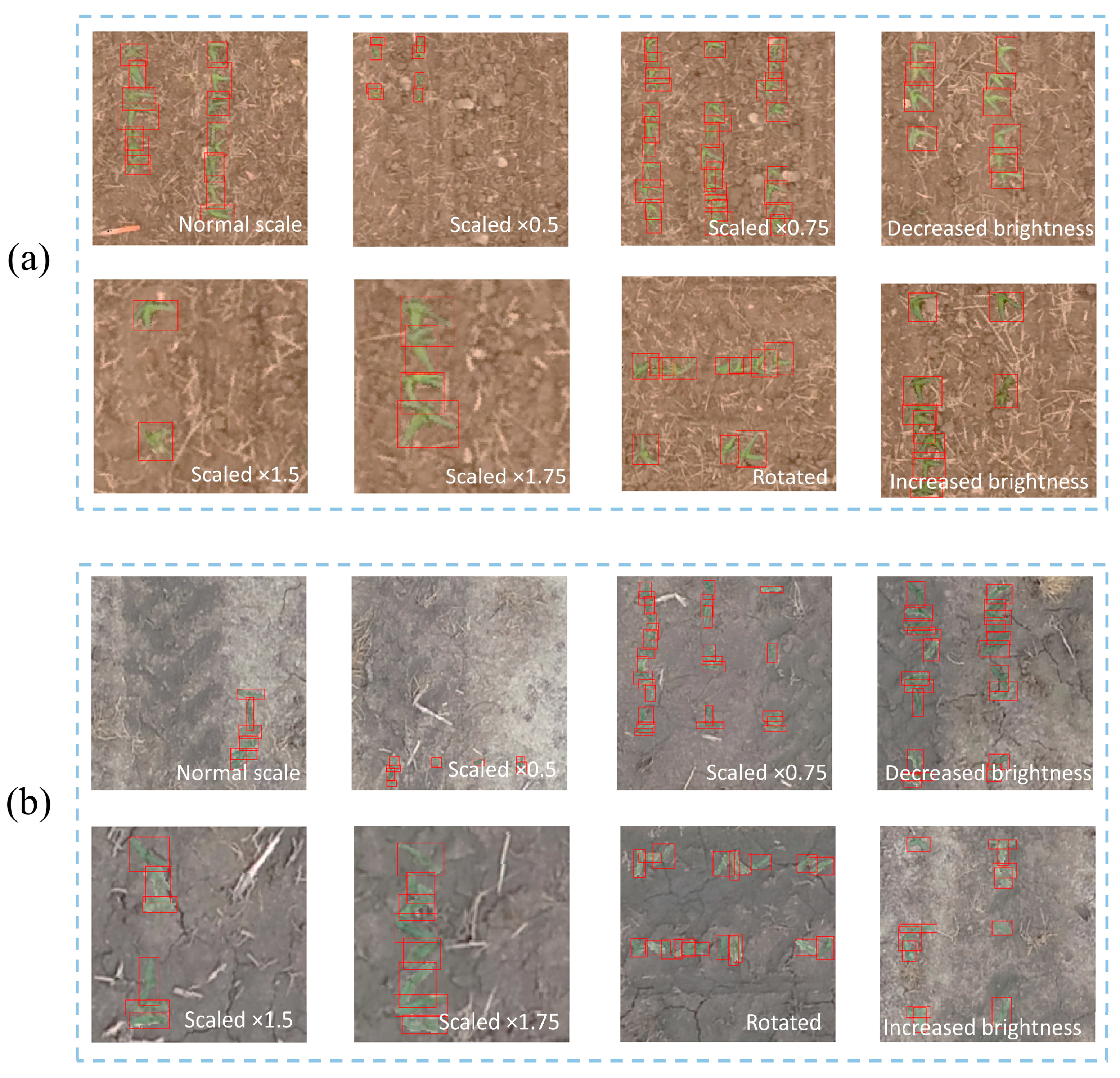
2.1. Training Data Generation
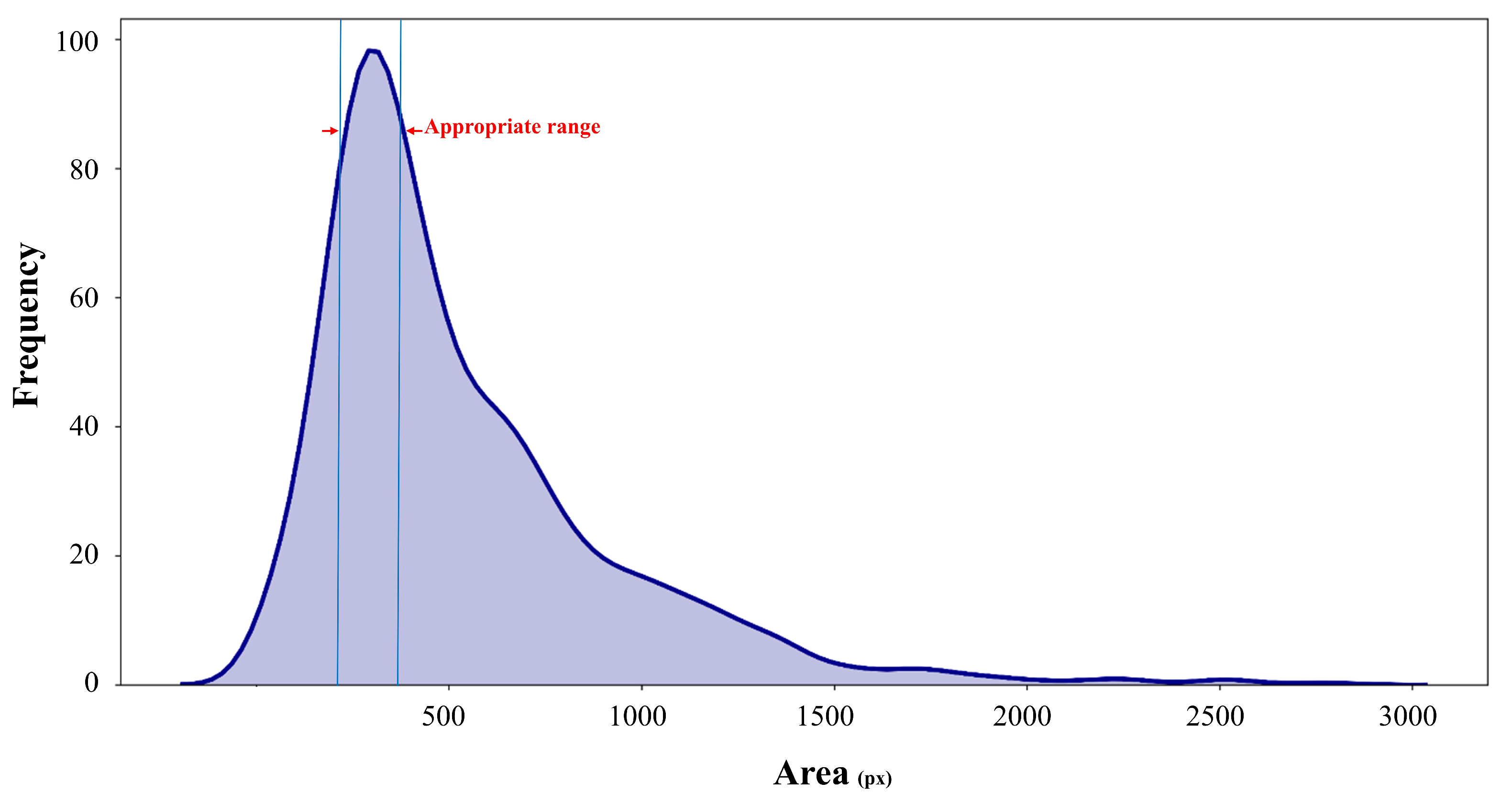
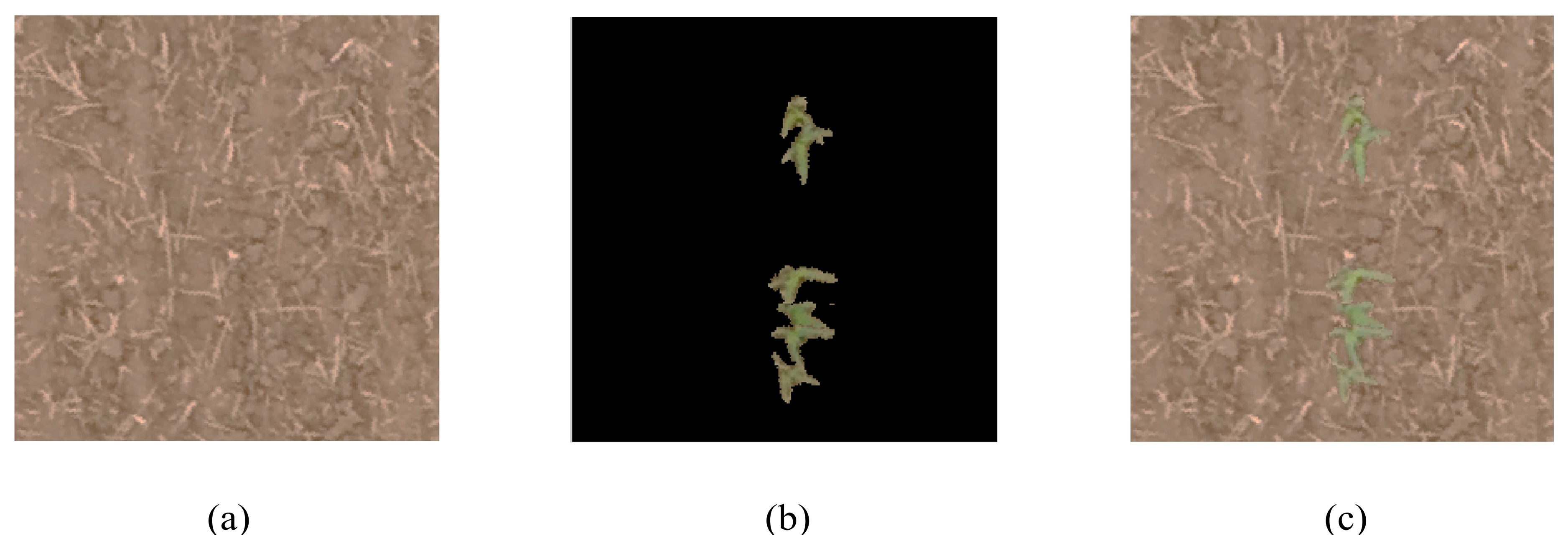
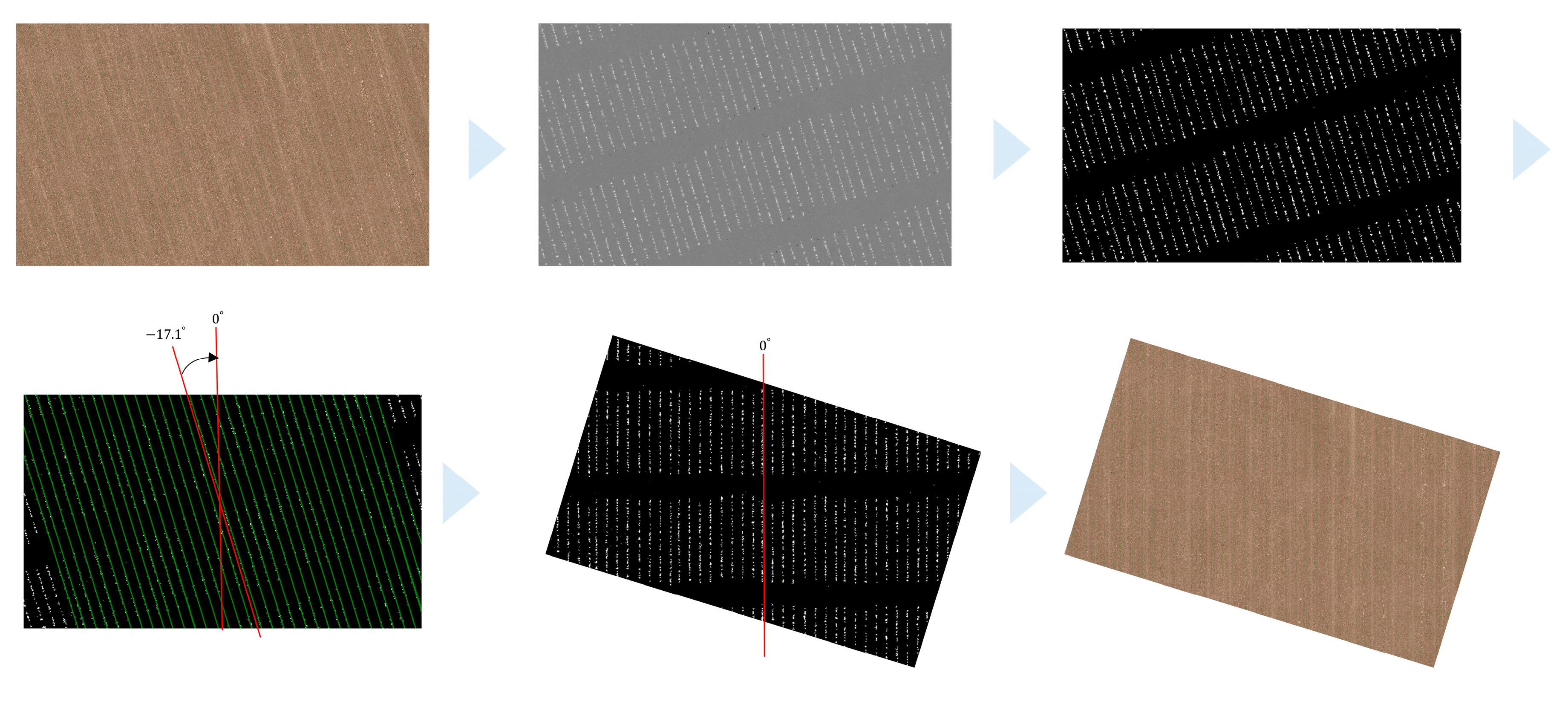
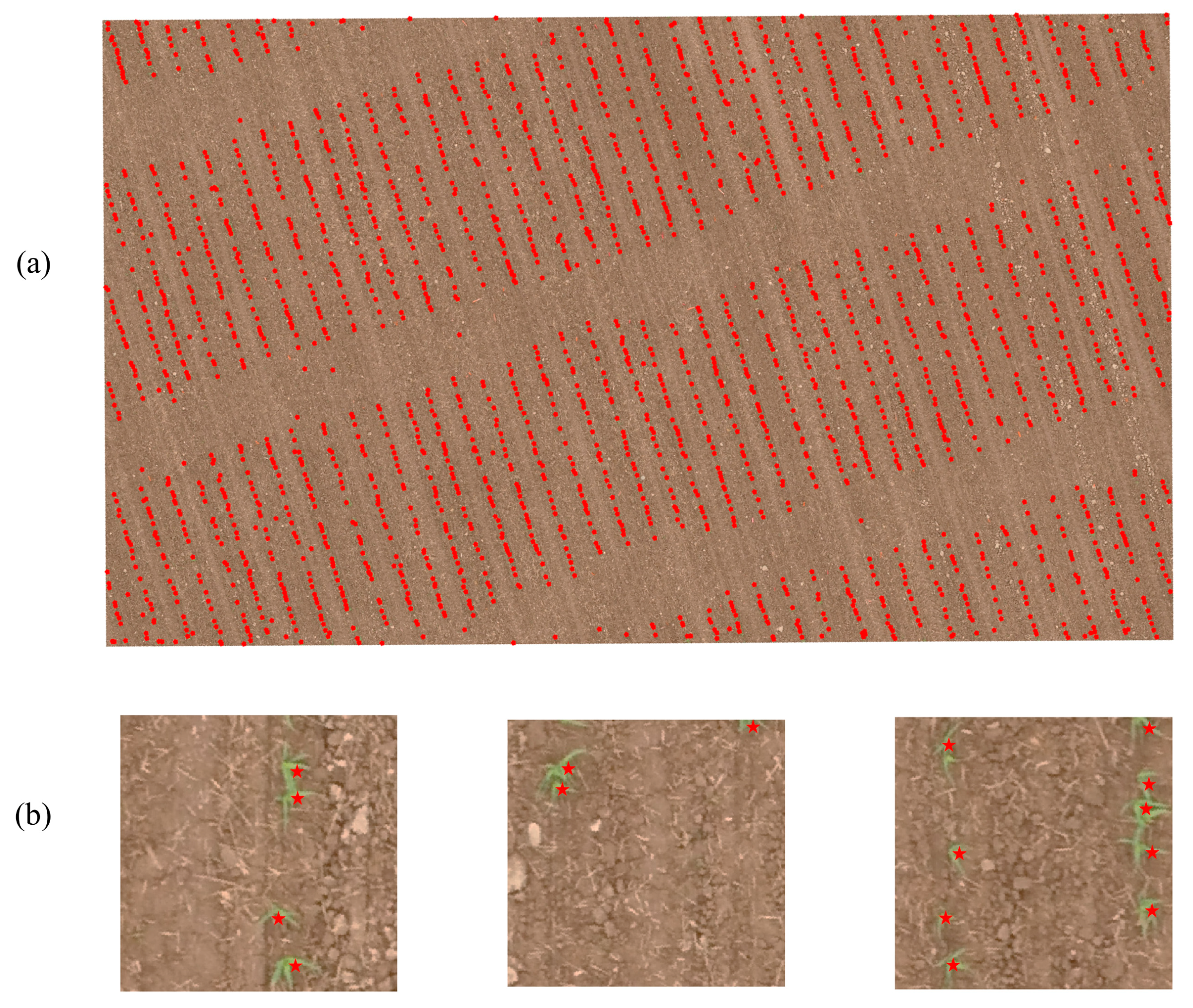
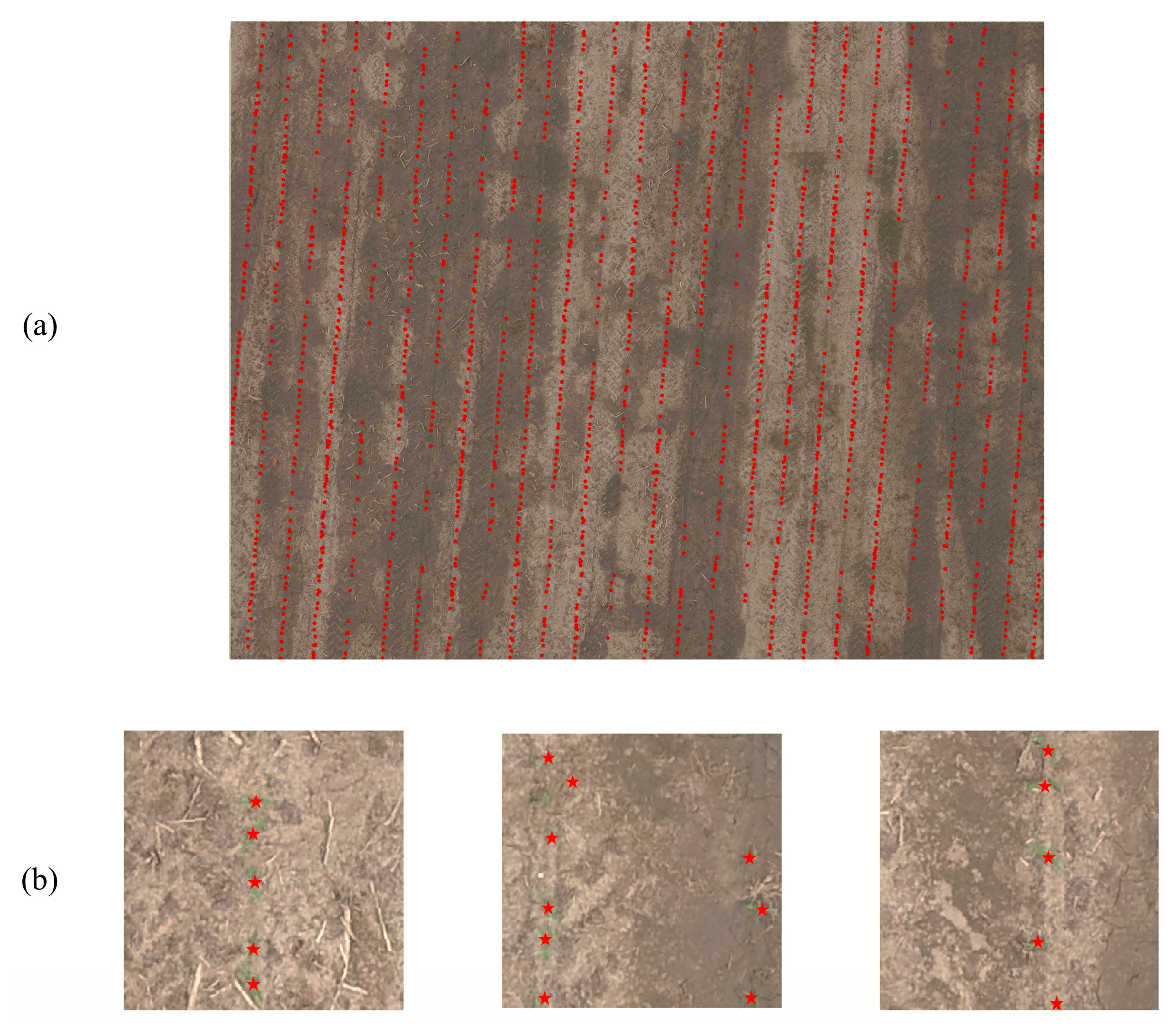
2.1.1. Automatic Sample Collection
2.1.2. Training Patch Generation
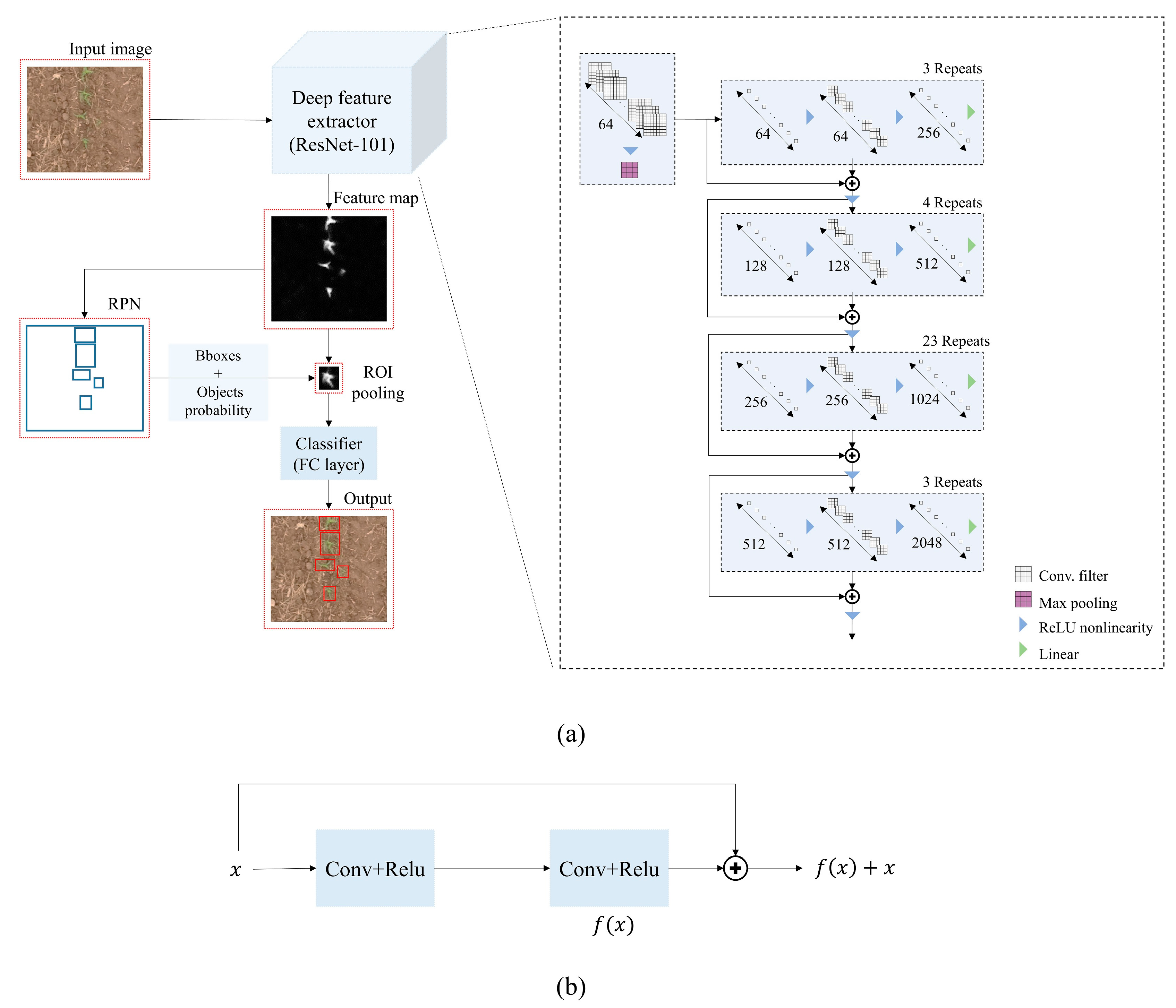
2.2. Deep Model Framework
2.3. Plant Detection
2.4. Evaluation Metrics
3. Experiments and Results
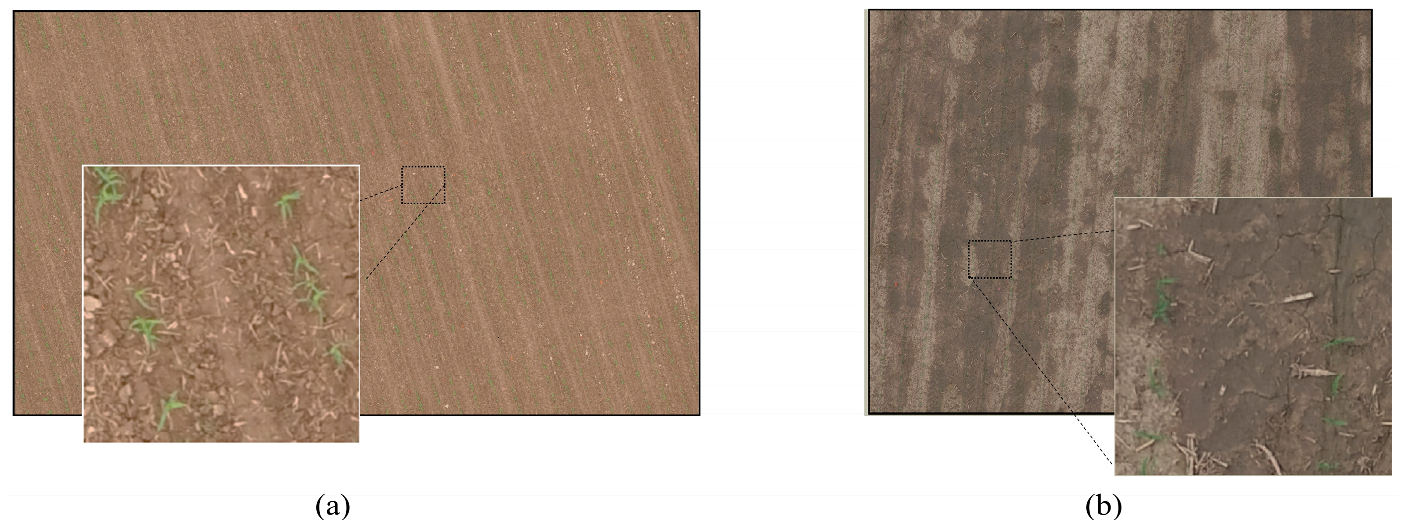
3.1. Drone Imagery
3.2. Implementation
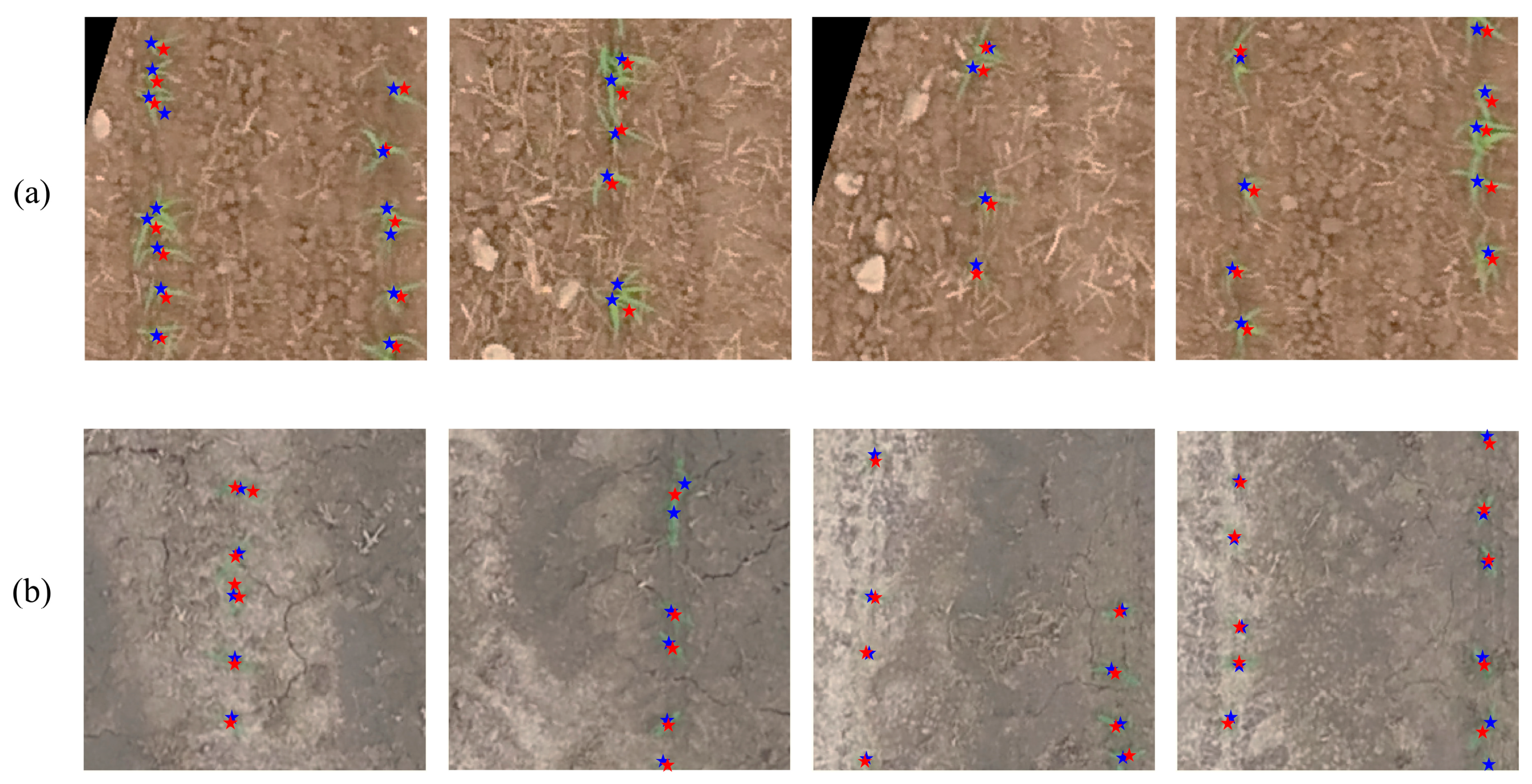
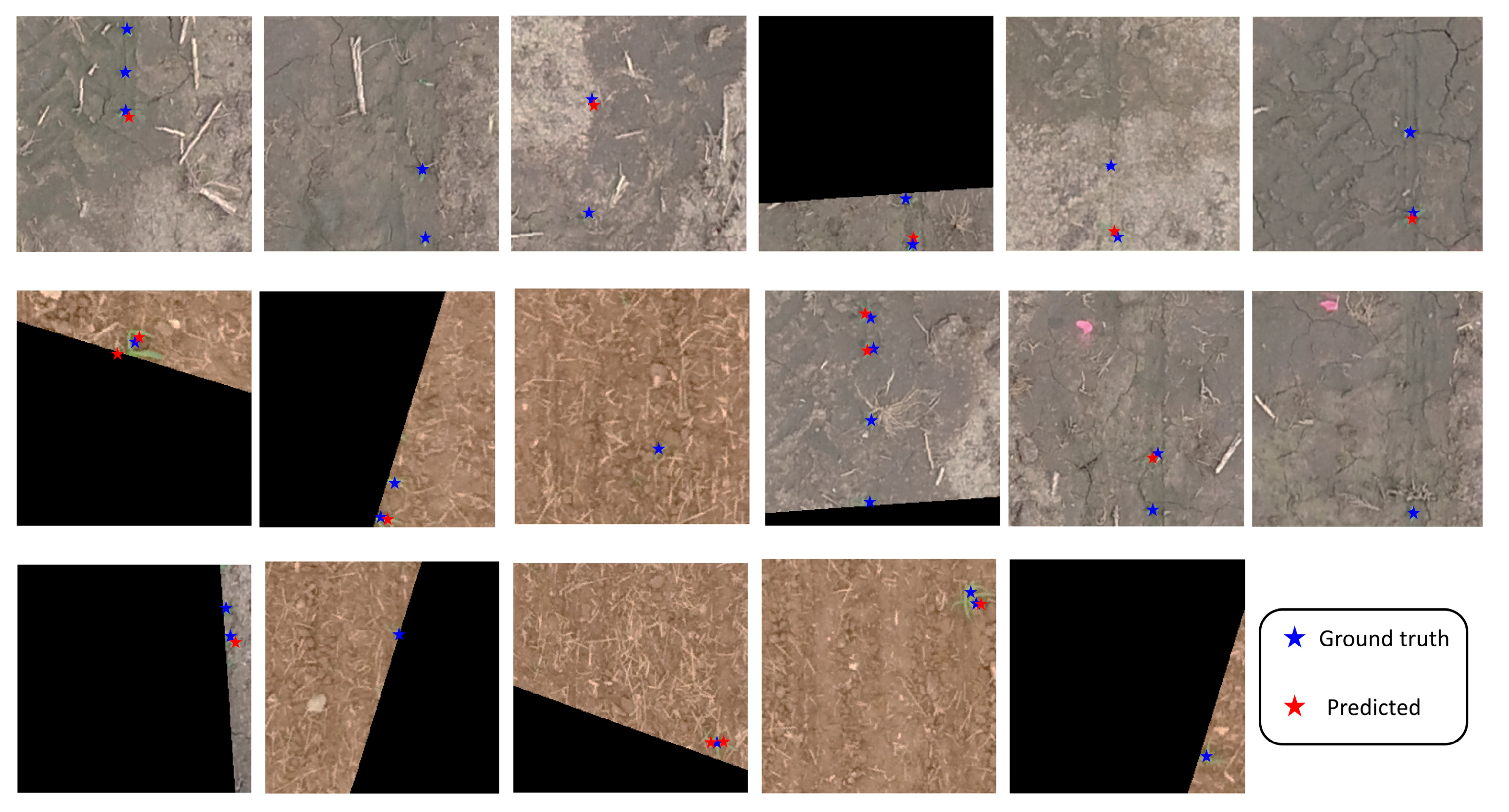
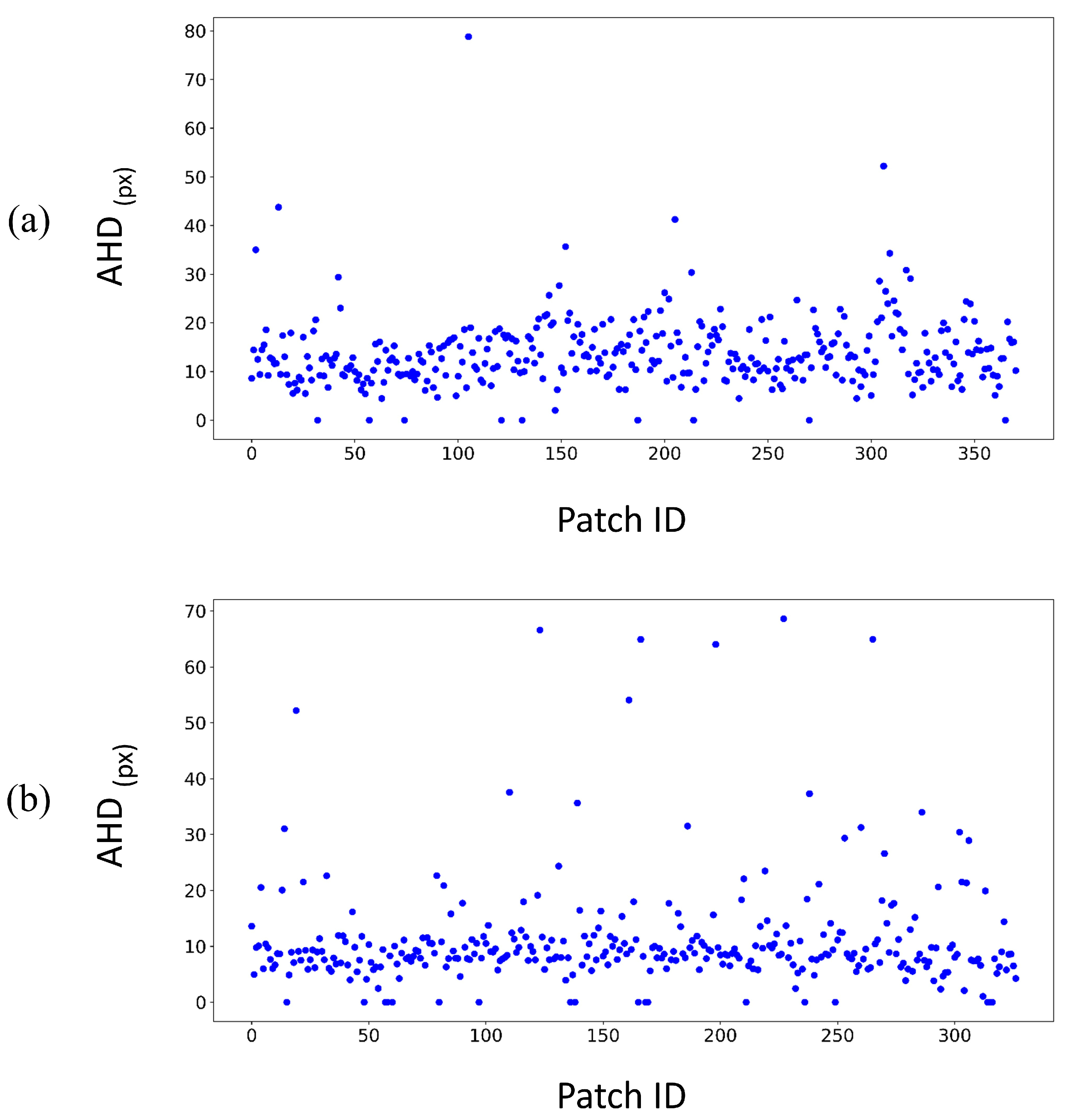
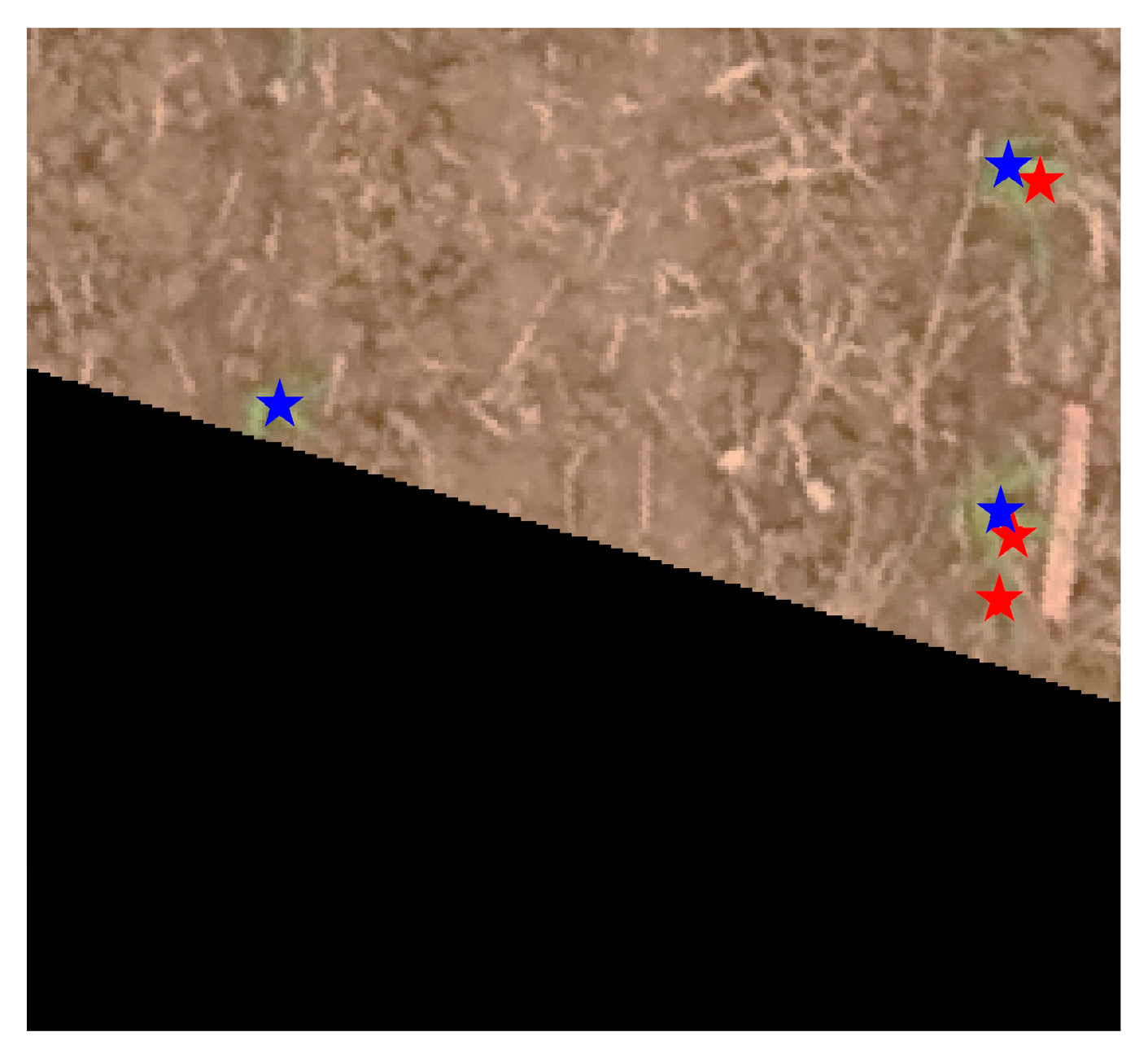
3.3. Results
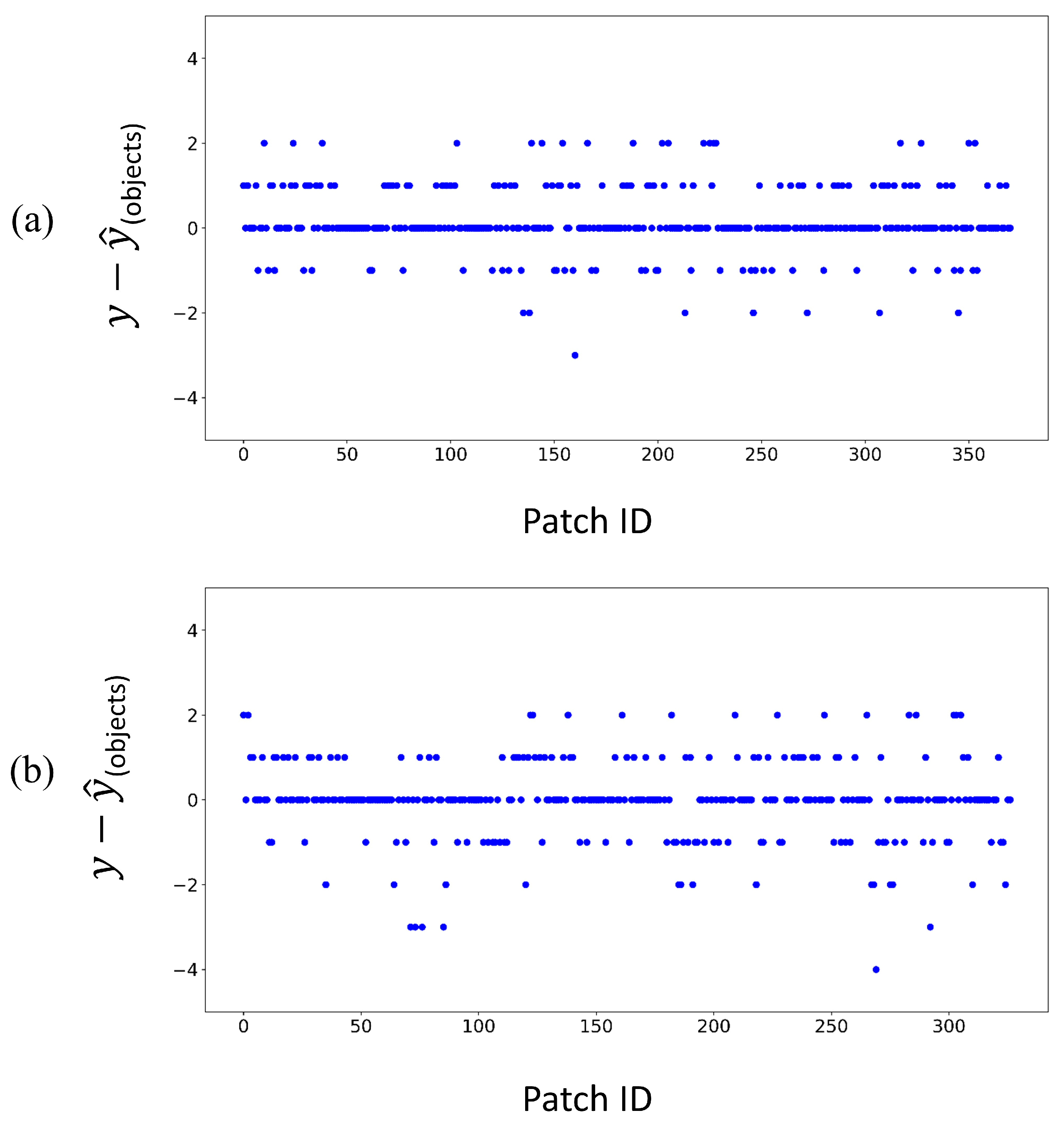
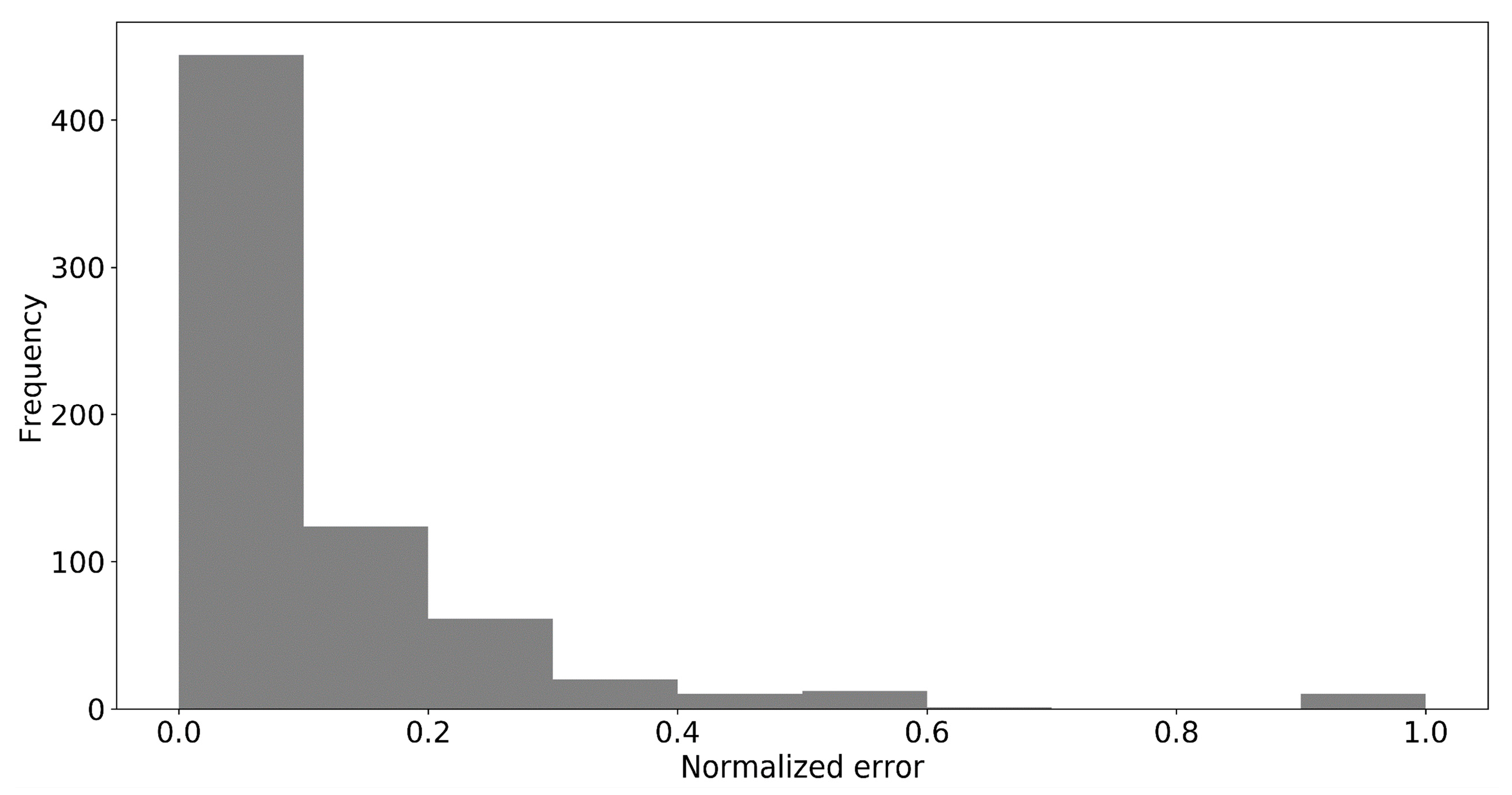
3.4. Accuracy Assessment
4. Discussion
4.1. In-Depth Evaluation of the Results
4.2. Challenges and Future Works
5. Conclusions
Author Contributions
Funding
Conflicts of Interest
References
- Godfray, H.C.J.; Beddington, J.R.; Crute, I.R.; Haddad, L.; Lawrence, D.; Muir, J.F.; Pretty, J.; Robinson, S.; Thomas, S.M.; Toulmin, C. Food security: The challenge of feeding 9 billion people. Science 2010, 327, 812–818. [Google Scholar] [CrossRef] [PubMed]
- Gikunda, P.; Jouandeau, N. State-Of-The-Art Convolutional Neural Networks for Smart Farms: A Review. In Proceedings of the Science and Information (SAI) Conference, London, UK, 18–20 July 2017. [Google Scholar]
- Seelan, S.K.; Laguette, S.; Casady, G.M.; Seielstad, G.A. Remote sensing applications for precision agriculture: A learning community approach. Remote Sens. Environ. 2003, 88, 157–169. [Google Scholar] [CrossRef]
- Kerkech, M.; Hafiane, A.; Canals, R. Deep leaning approach with colorimetric spaces and vegetation indices for vine diseases detection in UAV images. Comput. Electron. Agric. 2018, 155, 237–243. [Google Scholar] [CrossRef]
- Mulla, D.J. Twenty five years of remote sensing in precision agriculture: Key advances and remaining knowledge gaps. Biosyst. Eng. 2013, 114, 358–371. [Google Scholar] [CrossRef]
- Servadio, P.; Verotti, M. Fuzzy clustering algorithm to identify the effects of some soil parameters on mechanical aspects of soil and wheat yield. Span. J. Agric. Res. 2018, 16, 5. [Google Scholar] [CrossRef]
- Zhao, H.; Yuan, Q.; Song, S.; Ding, J.; Lin, C.-L.; Liang, D.; Zhang, M. Use of Unmanned Aerial Vehicle Imagery and Deep Learning UNet to Extract Rice Lodging. Sensors 2019, 19, 3859. [Google Scholar] [CrossRef] [PubMed]
- Sankey, T.; Donager, J.; McVay, J.; Sankey, J.B. UAV lidar and hyperspectral fusion for forest monitoring in the southwestern USA. Remote Sens. Environ. 2017, 195, 30–43. [Google Scholar] [CrossRef]
- Lottes, P.; Khanna, R.; Pfeifer, J.; Siegwart, R.; Stachniss, C. UAV-based crop and weed classification for smart farming. In Proceedings of the IEEE International Conference on Robotics and Automation, Singapore, 29 May–3 June 2017. [Google Scholar]
- Xiang, H.; Tian, L. Development of a low-cost agricultural remote sensing system based on an autonomous unmanned aerial vehicle (UAV). Biosyst. Eng. 2011, 108, 174–190. [Google Scholar] [CrossRef]
- Jin, X.; Liu, S.; Baret, F.; Hemerlé, M.; Comar, A. Estimates of plant density of wheat crops at emergence from very low altitude UAV imagery. Remote Sens. Environ. 2017, 198, 105–114. [Google Scholar] [CrossRef]
- Walter, A.; Khanna, R.; Lottes, P.; Stachniss, C.; Siegwart, R.; Nieto, J.; Liebisch, F. Flourish-a robotic approach for automation in crop management. In Proceedings of the International Conference on Precision Agriculture (ICPA), Montreal, QC, Canada, 24–27 June 2018. [Google Scholar]
- Mukherjee, A.; Misra, S.; Raghuwanshi, N.S. A survey of unmanned aerial sensing solutions in precision agriculture. J. Netw. Comput. Appl. 2019, 148, 102461. [Google Scholar] [CrossRef]
- Zhu, X.X.; Tuia, D.; Mou, L.; Xia, G.-S.; Zhang, L.; Xu, F.; Fraundorfer, F. Deep Learning in Remote Sensing: A Comprehensive Review and List of Resources. IEEE Geosci. Remote Sens. Mag. 2017, 5, 8–36. [Google Scholar] [CrossRef]
- Gong, M.; Yang, H.; Zhang, P. Feature learning and change feature classification based on deep learning for ternary change detection in SAR images. ISPRS J. Photogramm. Remote Sens. 2017, 129, 212–225. [Google Scholar] [CrossRef]
- Hosseiny, B.; Rastiveis, H.; Daneshtalab, S. Hyperspectral image classification by exploiting convolutional neural networks. Int. Arch. Photogramm. Remote Sens. Spat. Inf. Sci. 2019, 42, 535–540. [Google Scholar] [CrossRef]
- Hosseiny, B.; Shah-Hosseini, R. A hyperspectral anomaly detection framework based on segmentation and convolutional neural network algorithms. Int. J. Remote Sens. 2020, 41, 6946–6975. [Google Scholar] [CrossRef]
- Kamilaris, A.; Prenafeta-Boldú, F.X. Deep learning in agriculture: A survey. Comput. Electron. Agric. 2018, 147, 70–90. [Google Scholar] [CrossRef]
- Koirala, A.; Walsh, K.B.; Wang, Z.; McCarthy, C. Deep learning—Method overview and review of use for fruit detection and yield estimation. Comput. Electron. Agric. 2019, 162, 219–234. [Google Scholar] [CrossRef]
- Dijkstra, K.; van de Loosdrecht, J.; Schomaker, L.R.B.; Wiering, M.A. Centroidnet: A deep neural network for joint object localization and counting. In Machine Learning and Knowledge Discovery in Databases. ECML PKDD 2018; Lecture Notes in Computer Science; Springer: Dublin, Ireland, 2018; Volume 11053 LNAI, pp. 585–601. [Google Scholar]
- Wu, J.; Yang, G.; Yang, X.; Xu, B.; Han, L.; Zhu, Y. Automatic counting of in situ rice seedlings from UAV images based on a deep fully convolutional neural network. Remote Sens. 2019, 11, 691. [Google Scholar] [CrossRef]
- Ribera, J.; Guera, D.; Chen, Y.; Delp, E.J. Locating objects without bounding boxes. In Proceedings of the IEEE Conference on Computer Vision and Pattern Recognition, Long Beach, CA, USA, 15–20 June 2019; pp. 6479–6489. [Google Scholar]
- Attouch, H.; Lucchetti, R.; Wets, R.J.-B. The topology of theρ-hausdorff distance. Ann. Mat. Pura Appl. 1991, 160, 303–320. [Google Scholar] [CrossRef]
- Bellocchio, E.; Ciarfuglia, T.A.; Costante, G.; Valigi, P. Weakly Supervised Fruit Counting for Yield Estimation Using Spatial Consistency. IEEE Robot. Autom. Lett. 2019, 4, 2348–2355. [Google Scholar] [CrossRef]
- Osco, L.P.; de Arruda, M.d.S.; Marcato Junior, J.; da Silva, N.B.; Ramos, A.P.M.; Moryia, É.A.S.; Imai, N.N.; Pereira, D.R.; Creste, J.E.; Matsubara, E.T.; et al. A convolutional neural network approach for counting and geolocating citrus-trees in UAV multispectral imagery. ISPRS J. Photogramm. Remote Sens. 2020, 160, 97–106. [Google Scholar] [CrossRef]
- Girshick, R.; Donahue, J.; Darrell, T.; Malik, J. Rich feature hierarchies for accurate object detection and semantic segmentation. In Proceedings of the IEEE Conference on Computer Vision and Pattern Recognition, Columbus, OH, USA, 23–28 June 2014; pp. 580–587. [Google Scholar]
- Girshick, R. Fast r-cnn. In Proceedings of the IEEE International Conference on Computer Vision, Santiago, Chile, 7–13 December 2015; pp. 1440–1448. [Google Scholar]
- Ren, S.; He, K.; Girshick, R.; Sun, J. Faster R-CNN: Towards Real-Time Object Detection with Region Proposal Networks. In Advances in Neural Information Processing Systems; 2015; pp. 91–99. Available online: papers.nips.cc/paper/5638-faster-r-cnn-towards-real-time-object-detection-with-region-proposal-networks (accessed on 26 October 2020).
- He, K.; Gkioxari, G.; Dollár, P.; Girshick, R. Mask r-cnn. In Proceedings of the IEEE International Conference on Computer Vision, Venice, Italy, 22–29 October 2017; pp. 2961–2969. [Google Scholar]
- Redmon, J.; Divvala, S.; Girshick, R.; Farhadi, A. You only look once: Unified, real-time object detection. In Proceedings of the IEEE Conference on Computer Vision and Pattern Recognition, Las Vegas, NV, USA, 27–30 June 2016; pp. 779–788. [Google Scholar]
- Redmon, J.; Farhadi, A. YOLO9000: Better, faster, stronger. In Proceedings of the IEEE Conference on Computer Vision and Pattern Recognition, Honolulu, HI, USA, 21–26 July 2017; pp. 7263–7271. [Google Scholar]
- Redmon, J.; Farhadi, A. Yolov3: An incremental improvement. arXiv 2018, arXiv:1804.02767. [Google Scholar]
- Simonyan, K.; Zisserman, A. Very deep convolutional networks for large-scale image recognition. arXiv 2014, arXiv:1409.1556. [Google Scholar]
- He, K.; Zhang, X.; Ren, S.; Sun, J. Deep residual learning for image recognition. In Proceedings of the IEEE Conference on Computer Vision and Pattern Recognition, Las Vegas, NV, USA, 27–30 June 2016; pp. 770–778. [Google Scholar]
- Sa, I.; Ge, Z.; Dayoub, F.; Upcroft, B.; Perez, T.; McCool, C. DeepFruits: A Fruit Detection System Using Deep Neural Networks. Sensors 2016, 16, 1222. [Google Scholar] [CrossRef] [PubMed]
- Zhou, C.; Ye, H.; Hu, J.; Shi, X.; Hua, S.; Yue, J.; Xu, Z.; Yang, G. Automated Counting of Rice Panicle by Applying Deep Learning Model to Images from Unmanned Aerial Vehicle Platform. Sensors 2019, 19, 3106. [Google Scholar] [CrossRef]
- Rahnemoonfar, M.; Sheppard, C. Deep count: Fruit counting based on deep simulated learning. Sensors 2017, 17, 905. [Google Scholar] [CrossRef] [PubMed]
- Bah, M.; Hafiane, A.; Canals, R. Deep Learning with Unsupervised Data Labeling for Weed Detection in Line Crops in UAV Images. Remote Sens. 2018, 10, 1690. [Google Scholar] [CrossRef]
- Lin, T.-Y.; Maire, M.; Belongie, S.; Hays, J.; Perona, P.; Ramanan, D.; Dollár, P.; Zitnick, C.L. Microsoft coco: Common objects in context. In Proceedings of the European Conference on Computer Vision; Springer: Zurich, Switzerland, 2014; pp. 740–755. [Google Scholar]
- Deng, J.; Dong, W.; Socher, R.; Li, L.-J.; Li, K.; Fei-Fei, L. Imagenet: A large-scale hierarchical image database. In Proceedings of the 2009 IEEE Conference on Computer Vision and Pattern Recognition, Miami, FL, USA, 20–25 June 2009; IEEE: New York, NY, USA, 2009; pp. 248–255. [Google Scholar]
- Ding, J.; Chen, B.; Liu, H.; Huang, M. Convolutional neural network with data augmentation for SAR target recognition. IEEE Geosci. Remote Sens. Lett. 2016, 13, 364–368. [Google Scholar] [CrossRef]
- Wachowiak, M.P.; Walters, D.F.; Kovacs, J.M.; Wachowiak-Smolíková, R.; James, A.L. Visual analytics and remote sensing imagery to support community-based research for precision agriculture in emerging areas. Comput. Electron. Agric. 2017, 143, 149–164. [Google Scholar] [CrossRef]
- Theodoridis, S.; Koutroumbas, K. Pattern Recognition; Academic Press: Cambridge, MA, USA, 2009; ISBN 9780080949123. [Google Scholar]
- Goodfellow, I.; Bengio, Y.; Courville, A. Deep Learning; MIT Press: Cambridge, MA, USA, 2016; ISBN 0262337371. [Google Scholar]
- Rahnemoonfar, M.; Dobbs, D.; Yari, M.; Starek, M.J. DisCountNet: Discriminating and counting network for real-time counting and localization of sparse objects in high-resolution UAV imagery. Remote Sens. 2019, 11, 1128. [Google Scholar] [CrossRef]
- Duda, R.O.; Hart, P.E. Use of the Hough transformation to detect lines and curves in pictures. Commun. ACM 1972, 15, 11–15. [Google Scholar] [CrossRef]
- Rastiveis, H.; Shams, A.; Sarasua, W.A.; Li, J. Automated extraction of lane markings from mobile LiDAR point clouds based on fuzzy inference. ISPRS J. Photogramm. Remote Sens. 2020, 160, 149–166. [Google Scholar] [CrossRef]
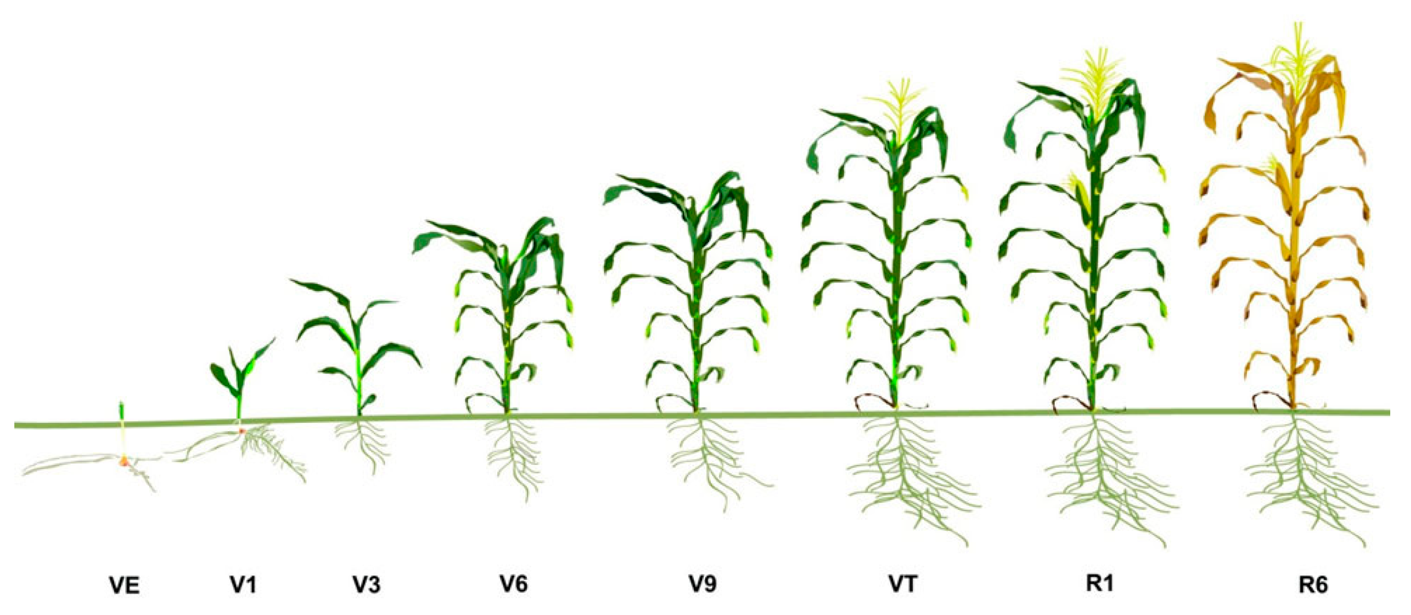
- Staging Corn Growth|Pioneer Seeds. Available online: https://www.pioneer.com/us/agronomy/staging_corn_growth.html (accessed on 18 October 2020).
- Sun, S.; Li, C.; Paterson, A.H.; Chee, P.W.; Robertson, J.S. Image processing algorithms for infield single cotton boll counting and yield prediction. Comput. Electron. Agric. 2019, 166, 104976. [Google Scholar] [CrossRef]
- Giuffrida, M.V.; Doerner, P.; Tsaftaris, S.A. Pheno-Deep Counter: A unified and versatile deep learning architecture for leaf counting. Plant J. 2018, 96, 880–890. [Google Scholar] [CrossRef] [PubMed]
- Itzhaky, Y.; Farjon, G.; Khoroshevsky, F.; Shpigler, A.; Bar-Hillel, A. Leaf counting: Multiple scale regression and detection using deep CNNs. In Proceedings of the BMVC, Newcastle, UK, 3–6 September 2018; p. 328. [Google Scholar]


| Convolutional Block | Number of Repeats | Kernels | Number of Filters |
|---|---|---|---|
| #1 Simple convolutional block | 1 | (7 × 7) | 64 |
| (3 × 3) | Max pooling | ||
| #2 Residual block | 3 | (1 × 1) | 64 |
| (3 × 3) | 64 | ||
| (1 × 1) | 256 | ||
| #3 Residual block | 4 | (1 × 1) | 128 |
| (3 × 3) | 128 | ||
| (1 × 1) | 512 | ||
| #4 Residual block | 23 | (1 × 1) | 256 |
| (3 × 3) | 256 | ||
| (1 × 1) | 1024 | ||
| #5 Residual block | 3 | (1 × 1) | 512 |
| (3 × 3) | 512 | ||
| (1 × 1) | 2048 |
| Camera Model | Flight Height (m) | Spectral Bands | GSD (cm) | ISO | Exposure Time (s) | Focal Length (mm) |
|---|---|---|---|---|---|---|
| FC6310 | 30 | R-G-B | 0.8 | 200 | 1/1250 | 9 |
| Simulation Type | Generated Samples |
|---|---|
| Normal-sized objects | 400 |
| Scaled objects (×0.5) | 50 |
| Scaled objects (×0.75) | 50 |
| Scaled objects (×1.5) | 50 |
| Scaled objects (×1.75) | 50 |
| Rotated object ordering | 100 |
| Object brightness changed (brightness increased between 10 and 30) | 50 |
| Object brightness changed (brightness increased between 30 and 10) | 50 |
| Total: | 800 samples |
| Dataset | Number of Patches | Average Number of Plants per Patch | MAE | Accuracy (%) | Mean AHD (Pixels) |
|---|---|---|---|---|---|
| Dataset 1 | 442 | 6.65 | 0.253 | 92.4 | 11.51 |
| Dataset 2 | 328 | 5.68 | 0.571 | 89.4 | 10.98 |
| Radius | Dataset | Mean Precision (×100) | Mean Recall (×100) | Mean F1 (×100) |
|---|---|---|---|---|
| R = 5 px | Dataset 1 | 71.49 | 71.14 | 71.20 |
| Dataset 2 | 72.63 | 71.69 | 71.76 | |
| R = 10 px | Dataset 1 | 73.76 | 73.42 | 73.39 |
| Dataset 2 | 80.87 | 79.31 | 79.51 | |
| R = 15 px | Dataset 1 | 79.41 | 78.95 | 79.00 |
| Dataset 2 | 86.06 | 83.32 | 84.21 | |
| R = 20 px | Dataset 1 | 84.52 | 83.90 | 84.05 |
| Dataset 2 | 89.04 | 85.89 | 87.00 |
| Study | Object Detector | Dataset | Training | Counting Results |
|---|---|---|---|---|
| [37] | Modified Inception-ResNet | 100 real images from Google | 24,000 simulated images | ACC = 0.9103 |
| RMSE = 2.52 | ||||
| [22] | FCN | 5000 patches from UAV scene | 80% training (5000 patches) | ACC: 0.958 |
| MAE: 1.9 | ||||
| AHD: 7.1 px (0.75 cm) | ||||
| [22] | Faster R-CNN | 5000 patches from UAV scene | 80% training (5000 patches) | ACC: 0.823 |
| MAE: 9.4 | ||||
| AHD: 9.0 px (0.75 cm) | ||||
| [21] | Two FCNs | 40 UAV scenes, each scene more than 10,000 plants | 900 patches of size 512 × 512 | ACC: 0.8194 |
| MAE: 1600/scene | ||||
| [50] | Feature fusion of MLP networks | 128 images | 50% training | MAE = 0.48 |
| [51] | CNN + MLP | 800 images | 80% training | MAE = 0.83 |
| [49] | Image processing | 210 images | Automatic | ACC = 0.846 |
| RMSE = 7.4 | ||||
| [24] | FCN encoder–decoder based on ResNet-101 | Camera images | 3000 image patches of size 300 × 300 | RMSE = 1.69~3.4 |
| [25] | FCN | Multispectral UAV | 80% training (448 patches of 256 × 256) | MAE = 2.05 |
| RMSE = 2.96 | ||||
| Our Method | Faster R-CNN | UAV scene | 800 simulated patches of size 256 × 256 | ACC: 0.89~0.92 |
| MAE: 0.25~0.57 | ||||
| AHD: 10.98~11.51 |
Publisher’s Note: MDPI stays neutral with regard to jurisdictional claims in published maps and institutional affiliations. |
© 2020 by the authors. Licensee MDPI, Basel, Switzerland. This article is an open access article distributed under the terms and conditions of the Creative Commons Attribution (CC BY) license (http://creativecommons.org/licenses/by/4.0/).
Share and Cite
Hosseiny, B.; Rastiveis, H.; Homayouni, S. An Automated Framework for Plant Detection Based on Deep Simulated Learning from Drone Imagery. Remote Sens. 2020, 12, 3521. https://doi.org/10.3390/rs12213521
Hosseiny B, Rastiveis H, Homayouni S. An Automated Framework for Plant Detection Based on Deep Simulated Learning from Drone Imagery. Remote Sensing. 2020; 12(21):3521. https://doi.org/10.3390/rs12213521
Chicago/Turabian StyleHosseiny, Benyamin, Heidar Rastiveis, and Saeid Homayouni. 2020. "An Automated Framework for Plant Detection Based on Deep Simulated Learning from Drone Imagery" Remote Sensing 12, no. 21: 3521. https://doi.org/10.3390/rs12213521
APA StyleHosseiny, B., Rastiveis, H., & Homayouni, S. (2020). An Automated Framework for Plant Detection Based on Deep Simulated Learning from Drone Imagery. Remote Sensing, 12(21), 3521. https://doi.org/10.3390/rs12213521