Abstract
A synthetic aperture radar (SAR) system can be seriously contaminated by radio frequency systems because of working in the same microwave frequency bands, which would degrade the SAR image quality and affect the accuracy of image interpretation. In this paper, a novel radio frequency interference (RFI) suppression approach including RFI identification, band-stop filtering and a removed spectrum iterative adaptive approach (RSIAA) is proposed. First, the smoothing process is added before RFI signal detection to improve the RFI detection capacity. Afterwards, the band-stop filtering with a broaden factor is proposed to mitigate the residual RFI, and it ensures the accuracy of the following removed spectrum recovery by the RSIAA. Finally, the removed spectrum components are estimated from available adjacent spectrum data by the RSIAA in turn to obtain the desired range spectra. Compared with the conventional range frequency filtering method for RFI suppression, the capacity of the weak RFI signal detection is improved, and the increased sidelobes due to the discontinuous spectra are well suppressed. Simulation experiments on both simulated SAR raw data, Gaofen-3 and Sentinel-1 SAR raw data validate the proposed RFI suppression approach.
1. Introduction
Synthetic aperture radar (SAR) is an active microwave remote sensing instrument for Earth’s surface observation, and it can be widely utilized in both military surveillance and civilian exploration [1]. However, in the more and more complex electromagnetic environment, the received SAR echoes are increasingly corrupted by radio frequency interferences (RFIs). Although SAR systems have an inherent capability of anti-interference, RFI signals with characteristics of a one-way propagation path and long working time can severely degrade the quality of the desired SAR images [2,3,4]. Commonly, typical RFI resources mainly come from networks, communication systems and other electromagnetic devices [5,6,7]. Hence, radio interference identification and suppression have attracted extensive attention in the SAR field.
According to the interference bandwidth to the SAR signal bandwidth ratio, RFI can be simply divided into narrow-band interference (NBI) and wide-band interference (WBI). The bandwidth of NBI is usually tens of kilohertz, while the WBI bandwidth is usually less than 10 MHz and much smaller than that of wideband SAR systems [8].
In recent years, RFI suppression approaches have been mainly categorized into two classes: parametric and nonparametric methods. In terms of the parametric approaches, the interferences are constructed as a sinusoidal model [9,10,11], and its amplitude, frequency and phase is estimated by the least mean square method [12,13,14] or the maximum likelihood approach [15]. The mathematical model is optimized under specific criteria [16,17,18,19], and the RFI can be extracted and subtracted from the received SAR echo signals. Commonly, the NBI is suppressed using the parametric methods because of the multiple generated sinc peaks in the frequency domain. Yi et al. [17] and Guo et al. [18] proposed an effective approach using the maximum a posterior (MAP) estimation for RFI suppression, but the approach depends on the precise prior knowledge. The RELAX algorithm is a signal parameter estimation method which estimates the target signal parameters by minimizing the nonlinear least square method, and this method can be used to estimate the RFI parameters. Huang et al. [11] proposed a gradual use of the RELAX algorithm, which can estimate the parameters for each frequency peak with a reduced number of estimation iterations of the traditional RELAX algorithm. Although parametric methods can accurately estimate the sinusoid model, these methods are restricted by some conditions, such as prior knowledge, computational complexity and precise model [20,21]. Unlike the parametric methods, the nonparametric methods implement RFI suppression without any prior knowledge or precise model, and the spectral characteristic is exploited to filter out RFI in the frequency or time–frequency domain. The NBI and WBI are mitigated by nonparametric methods based on the designed filters and constructed subspace projector. In [22], Zhou et al. proposed an eigenvalue subspace projection (ESP) method that constructs the NBI and signal subspaces by singular value decomposition (SVD) to suppress the interferences. The least mean square (LMS) filter was designed by Le et al. to adaptively mitigate interferences for single-channel SAR systems [23]. The band-stop filtering method is a typical nonparametric method, which designs a frequency notching filter to remove the interference that occupies a certain frequency band [24,25]. However, the interference is effectively suppressed by the band-stop filter, while the useful signal in the same frequency band is also removed, which results in multiple artifacts in the final SAR image.
In this paper, a novel RFI suppression method including RFI identification, frequency band-stop filtering and the removed spectrum iterative adaptive approach (RSIAA) is proposed. Firstly, the spectrum smoothing preprocess, which uses a sliding averaging window to reduce the spectrum dynamic range, is added to the conventional RFI detection in the frequency domain to ensure accurate RFI detection and identification. According to identified frequency parameters of detected RFI signals, the RFI signals can be removed by the designed band-stop filter. Taking account of the Gibbs effect in the digital Fourier transform (DFT), the small amount of residual RFI energy would not only affect the quality of the final SAR image but also degrade the accuracy of the following removed effective spectrum recovery. Hence, the bandwidth broadening factor for residual RFI energy mitigation is analyzed and designed. Then, the band-stop filter is conducted based on identified RFI frequency parameters and the bandwidth broadening factor. Unfortunately, part of the useful spectrum in the same frequency band is simultaneously removed with RFI signals, which will degrade the SAR image quality and is the major disadvantage of the band-stop filtering method. The iterative adaptive approach (IAA) [26] is an effective method for missing data amplitude estimation, and when it is introduced to recover the removed effective range spectrum it is named as the RSIAA. Finally, the removed spectrum amplitude is estimated by a weighted least squares criterion, and the missing data amplitude is reconstructed from the adjacent spectrum data. After that, the RFI energy is effectively mitigated by the band-stop filter, and the range spectrum is still consistent. The advantages of the proposed approach can be summarized in three aspects: (1) the more accurate weak RFI detection capacity after the spectrum smoothing process; (2) the better residual RFI suppression effect due to the introduced broadening factor; (3) the improved SAR image quality after the removed spectrum estimation by the IAA. Furthermore, since all these processing operations could be implemented by a pulse-by-pulse behavior, another important advantage of the proposed approach is the effectiveness to deal with the azimuth time-variant RFI signals.
The remainder of this paper is arranged as follows. In Section 2, the model of the interference signal is introduced, and the characteristics of different interferences are analyzed in the time and frequency domains. The RFI identification and removed spectrum recovery are presented in detail in Section 3. In Section 4, the proposed RFI suppression approach including RFI identification, band-stop filtering with a broadening factor and the RSIAA are described. Simulation experiments on simulated targets and real SAR data are carried out to validate the proposed approach in Section 5. Finally, this paper is discussed and concluded in Section 6 and Section 7.
For clarity, the main abbreviations used in this paper are listed in Table 1.

Table 1.
Main abbreviations.
2. Interference Formulation and Analysis
With the increase in modern electromagnetic devices and the overlapping utilization of the electromagnetic spectrum, the SAR system with a wide frequency bandwidth is severely affected by the interference of other electromagnetic radiation sources in the working frequency band and, in particular, the SAR signal is susceptible to complicated interferences, including NBIs and WBIs in practical scenarios.
For a single-channel SAR system, each echo received during a pulse repetition time can be formulated as
where denotes the range time sample, denotes the complex-valued radar pulse, indicates the desired target echoes, and are the RFI and additive noise, respectively. To generate an azimuth high-resolution SAR image, the received SAR signal is usually constructed into a two-dimensional (2D) time domain. Afterwards, the SAR signal in the range time and azimuth time is written as follows:
According to the narrow-band characteristics of RFI, it is assumed that the RFI signal is a superposition of a plurality of complex sinusoids [27], and the mathematical expression of narrow-bandwidth RFI is defined as
where Al is the amplitude envelope of the l-th RFI signal, fl and ϕl indicate the carrier frequency and the modulated phase of the l-th interference signal, respectively, and L is the number of RFI signals. There are usually two ways to modulate WBI signals. One is the chirp-modulated (CM) WBI, the other is the sinusoidal-modulated (SM) WBI [28,29]. These two forms can be expressed as
where is the amplitude envelope of the l-th RFI signal, and represent the carrier frequency and the chirp modulation rate, respectively, and are the modulation factor and the phase of the l-th interference component, respectively.
The received echoes are the superposition of echoes from multiple scatterings in the imaged scene, which makes the waveform of the received echoes disorganized in the range time domain. Hence, it is impossible to determine whether there is an RFI signal or not through the waveform of the time domain. Furthermore, since the bandwidth of the RFI signal is usually in the range of 0.1–10 MHz, the frequency bandwidth of the RFI signal is much smaller than the transmitted pulse bandwidth by SAR systems. The RFI detection is implemented in the frequency domain, and the received SAR data are transformed into the range–frequency azimuth time domain by the Fourier transform as:
where is the range frequency, is the number of samples and , , and denote the received echoes, NBI, WBI and additive noise, respectively.
According to simulation parameters of RFI signals listed in Table 2, Figure 1 shows illustrations of the NBI and WBI signals in different domains. In Figure 1a,b, both NBIs and WBIs are presented as bright lines along the range direction in the 2D time domain after SAR imaging process. If these bright lines are superimposed on an SAR image, there is no doubt that they will hinder the SAR image interpretation. Figure 1c shows the range spectrum of the NBI in the 2D frequency domain, which demonstrates that the NBI energy mainly concentrates on a few particular frequencies, and Figure 1d shows that the WBI occupies a large proportion of bandwidth. Since the RFI signal has characteristics of the one-way propagation path, long working time and narrow bandwidth, it has high power in the range frequency domain, as show in Figure 1e,f. Because of the Gibbs effect, the residual RFI may still exist after the conventional band-stop RFI suppression.
Table 2.
Simulation parameters of the experiments.
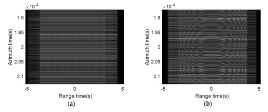
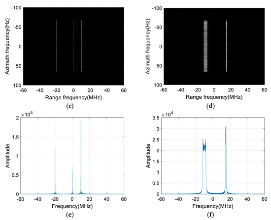
Figure 1.
NBI and WBI in different domains. (a) NBI in the 2D time domain; (b) WBI in the 2D time domain; (c) NBI in the 2D frequency domain; (d) WBI in the 2D frequency domain; (e) NBI in the range frequency domain; (f) WBI in the range frequency domain.
In order to analyze the influence of different intensities of RFI on SAR images, a focused SAR image of a city background is selected from a website [30]. Different interference to signal ratios (ISRs) are intentionally added to the simulated raw data of the city SAR image, and the imaging results are shown in Figure 2. Since the low-frequency band, such as L and P bands, is a common frequency band for both SAR and radio frequency systems, SAR signals in the low-frequency band are susceptible to RFI signals. Therefore, the L band is adopted in the following simulations [2,8], and the simulated RFI parameters are listed in Table 2. Figure 2a is the imaging result without any RFI signals for comparison, while Figure 2b–d shows imaging results of the SAR raw data with RFI signals at different intensities. The strong RFI is added in Figure 2b, and the high ISR is 10 dB and makes the whole SAR image unrecognizable. Figure 2c has the ISR of 5 dB, in which the RFI will obviously affect target identification, especially weak targets. The ISR in Figure 2d is 5 dB, in which the RFI may be considered well mitigated, but the small amount of residual RFI energy would result in some blurred stripes in the SAR image, especially for the areas with the low signal to noise ratio (SNR) level. The low ISR will not seriously affect SAR image applications for target identification, but it will degrade the accuracy of the detailed information description and extraction in SAR images, such as road extraction, building height estimation and detailed target information description.
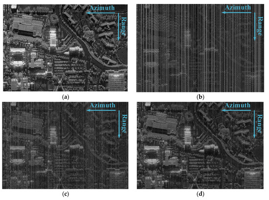
Figure 2.
Comparison of focused SAR images with different interference to signal ratios (ISRs). (a) Original SAR image; (b) ISR = 10 dB; (c) ISR = 5 dB; (d) ISR = −5 dB.
3. Theory
According to simulation results of the RFI signals presented in the time, frequency and image domains, as shown in Figure 1 and Figure 2, RFI identification and mitigation in the range frequency domain seem to be a reasonable choice. The major drawback of this operation is part of the effective spectrum of the desired scene is simultaneously removed by the range frequency band-stop filter. In order to improve the image quality, removed spectrum recovery is introduced from theory and designed experiments in this section.
3.1. RFI Identification
For an SAR system, echoes are always accompanied by strong RFI, but some indiscernibly weak RFIs are also contained in SAR raw data. In order to effectively and accurately suppress interference, we should accurately detect the RFI and recognize its carrier frequency and bandwidth in the frequency domain. Usually, the RFI signal is detected by a reasonable amplitude threshold for each range line in the frequency domain. If the range spectrum amplitude at some particular frequencies is larger than the designed amplitude threshold, echoes of this pulse are considered as contaminated by interferences. However, an appropriate threshold cannot be designed when the weak RFI is contained for SAR echo data with large vibration amplitude. For the accurate weak RFI identification and an appropriate threshold selection, the smoothing processing using a sliding window is carried out before RFI detection in the frequency domain.
After the smoothing processing by the sliding averaging window, the smoothed range spectrum is expressed as follows:
where is the original range spectrum and is the sample number of the sliding window for smoothing processing. In order to analyze the RFI detection capability, an experiment on multiple point targets is conducted. The designed WBI signals are added to the echoes and WBI simulation parameters are listed in Table 2. The amplitude threshold value is usually designed as the mean plus one to three times the standard deviation (δ) to detect the RFI signal and estimate its corresponding parameters such as bandwidth and carrier frequency.
The original spectrum is shown in Figure 3a,d,g, while RFI detection and parameter estimation become much more difficult due to the large dynamic range of the spectrum amplitude, especially for weak RFI. The smoothing operation is a classic method to reduce the dynamic range, and it can be implemented by an averaging window or data convolution. In this paper, an averaging window is adopted, and smoothing results by the averaging window with different sizes are shown in Figure 3. Compared with original spectra, RFI detection and parameter estimation become much easier, while RFI bandwidth estimation results are summarized in Table 3. According to results listed in Table 3, if the size of the chosen averaging window is too large, the estimation accuracy would be obviously reduced and even result in no RFI detected. The reason for this is that the bandwidth of the averaging window is larger than the one of the RFI signal. Therefore, a reasonable window size should be carefully designed according to characteristics of RFI signals. Furthermore, the threshold value will also affect the accuracy of estimation results. Compared with the other two threshold values, μ + 2δ is a better choice and adopted in the following simulation.
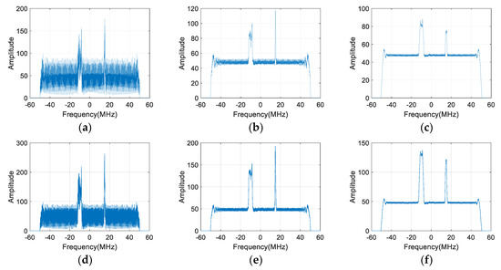
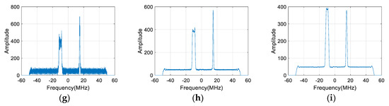
Figure 3.
Comparisons of the range spectrum smoothing results using different smoothing window sizes under different ISRs. (a) The original spectrum, ISR = −10 dB; (b) after 10 points smoothing, ISR = −10 dB; (c) after 30 points smoothing, ISR = −10 dB; (d) the original spectrum, ISR = −5 dB; (e) after 10 points smoothing, ISR = −5 dB; (f) after 30 points smoothing, ISR = −5 dB; (g) the original spectrum, ISR = 5 dB; (h) after 10 points smoothing, ISR = 5 dB; (i) after 30 points smoothing, ISR = 5 dB.
Table 3.
RFI bandwidth identification using different window sizes under different ISRs.
In this section, the averaging window is used to reduce the dynamic range of the range spectrum, and the purpose of the smoothing operation is to improve the RFI detection capacity and parameter estimation accuracy. The weak RFI cannot be detected by a low detection threshold, if the range spectrum has a large dynamic range and does not have any smoothing operation, as shown in Table 3. Furthermore, the narrow and weak RFI may also be ignored by the high-level detection threshold due to the over-smoothing operation.
A reasonable window size should be carefully designed according to characteristics of RFI signals. First, the large smoothing window is used for RFI detection with a large bandwidth, then the smaller smoothing window is adopted to ensure the weak RFI detection capacity. With this processing behavior, almost all RFI signals can be detected after the smoothing operation, although the estimated bandwidth of the RFI signals is not very accurate.
3.2. Removed Spectrum Iterative Adaptive Approach
After the RFI suppression by band-stop filtering, part of the effective spectrum is simultaneously removed with RFI signals, and the discontinuous range spectrum results in artifacts and increased sidelobes. The IAA is an effective interpolation method to recover missing data and is applied in multiple applications in the time domain [31]. In this paper, the discontinuous range spectrum is recovered by IAA, and this removed spectrum recovery approach is named as the RSIAA.
After the RFI mitigation and range matched filtering, the received complex-valued SAR range spectrum can be defined as , while the available and removed spectra are defined as the vectors and , respectively, as:
where denotes the range frequency of the available and effective spectrum, indicates the range frequency of the removed spectrum, denotes the number of effective grid points in the frequency domain, is the bandwidth of the SAR pulse. According to the range spectrum of the RFI signal in Figure 1, the removed range frequency samples are interleaved with the available frequency samples . Consequently, the removed spectrum recovery is transformed into an interpolation problem.
According to the digital Fourier transform (DFT), the range spectrum can be expressed as
with
where is the number of total samples in the time domain, denotes the complex-valued amplitude vector for the uniform sampled time vector and the vector is related to the complexity of the imaged scene.
For most imaged scenes, the vector is sparse, which means that many elements of the vector are quite small and even equal to zero. In such a sparse case, by using a weighted least squares criterion [26] and the matrix inversion lemma [32], the complex-valued amplitude can be estimated as follows:
where denotes the covariance matrix of the available data, is the conjugate transpose and denotes the matrix inversion. According to Equations (15)–(17), Equation (15) must be implemented in an iterative manner, and the initial value of could be set to the identity matrix.
Consequently, the removed range spectrum is estimated from the available spectrum data as follows [32]:
where
where the sizes of and are the same as and .
In order to validate the iterative adaptive approach to recover the removed range spectrum, simulation experiments with parameters listed in Table 2 are carried out. Three point targets are designed in the imaged scene, and the target relative range positions are 0 m, 300 m and 750 m, respectively, while their corresponding relative scattering intensities are 1, 0.5 and 0.8, respectively. The estimation ratio is defined as the ratio of the available data length to the removed data length . If the estimation ratio is too small, the missing spectrum cannot be recovered well, as shown in Figure 4c, which results in the increased sidelobes, as shown in Figure 4f–h.
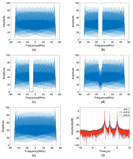
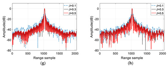
Figure 4.
Simulation results of the removed spectrum estimation. (a) The original spectrum; (b) the removed spectrum by band-stop filtering; (c) the estimation result of ; (d) the estimation result of ; (e) the estimation result of ; (f) comparison of range compression results; (g) interpolation results of the strongest target; (h) interpolation results of the weakest target.
The imaging performances, including peak side lobe ratio (PSLR) and integral side lobe ratio (ISLR) with different , are measured and summarized in Table 4. According to the results in Table 4, the larger brings better imaging performances, but it would consume much more computing resources and time.
Table 4.
The performances of different available data lengths for the same removed data recovery.
4. Methodology
According to the abovementioned analysis and simulation results, the RFI suppression approach based on the RSIAA is proposed, which includes three major processing steps: RFI identification, RFI band-stop filtering and removed spectrum estimation. The flow chart of the proposed approach is shown in Figure 5.
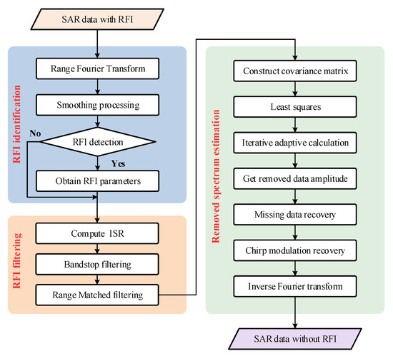
Figure 5.
Flow chart of the proposed RFI suppression approach.
According to simulation results in Figure 3, after smoothing processing via a moving average window, the dynamic range of the range spectrum is obviously reduced, and the RFI detection and parameter estimation including bandwidth and carrier frequency could be more accurately implemented. If the bandwidth of the band-stop filter is set to the detected bandwidth, the residual RFI energy due to the Gibbs effect will still degrade the image quality. Furthermore, the residual RFI energy will affect the following missing spectrum recovery by the IAA. Therefore, the band-stop filtering for RFI mitigation must have a broadened bandwidth.
The broadening factor is defined as the ratio of the bandwidth of the band-stop filter to the one of the detected RFI bandwidth. To discuss the value of the broadening factor , a simulation experiment on the point target is carried out. Figure 6 shows the removed spectrum estimation and range compression results with different broadening factors, and factor in Figure 6a,c are selected as 1 and 2, respectively. It can be seen that the residual RFI energy due to the Gibbs effect would obviously affect the removed spectrum recovery, and the recovered spectrum in Figure 6a results in high-level artifacts. After introducing the broadening factor , the removed spectrum is recovered well, and then the high-level sidelobes caused by the discontinuous range spectrum are obviously suppressed, as shown in Figure 6d.
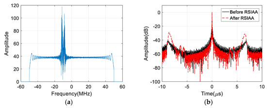
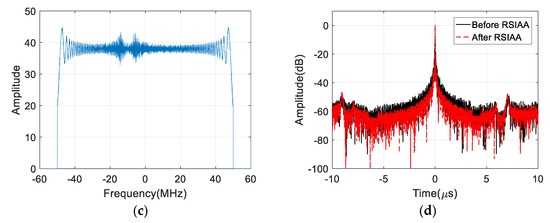
Figure 6.
Simulation results of and . (a) The recovered spectrum of ; (b) the pulse compression result of (a); (c) the recovered spectrum of ; (d) the pulse compression result of (c).
Moreover, imaging performances including resolution (Res.), PSLR and ISLR after the RSIAA with different broadening factors are measured and summarized in Table 5. According to the measured parameters listed in Table 5, PSLR and resolution are almost the same, but ISLR is significantly affected by the broadening factor. Commonly, the high ISLR level would lead to an increased noisy background in the focused SAR image.
Table 5.
The measured performances after the removed spectrum iterative adaptive approach (RSIAA) with different broadening factors.
The relationship between the broadening factor and the ISLR under different ISRs is shown in Figure 7. Ideally, the ISLR of the pulse compression result with rectangular weighting is about 10 dB. The high ISLR level is not tolerated in multiple SAR image applications. Therefore, only a very limited ISLR increase is permitted, and the referenced broadening factor could be obtained according to the acceptable ISLR level. According to Figure 7b, the minimum broadening factors for different ISLRs under different ISRs can be obtained. After taking interpolation and quadratic curve fitting as shown in Figure 8, the referenced broadening factor is obtained as:
when denotes the ISR, and it can be calculated from the echoes after RFI detection [28]. For different referenced ISLR values, the coefficients , and are obtained from quadratic curve fitting and listed in Table 6. In addition, the used broadening factor can be a little larger than the referenced value in practice, but one that is too large will consume more computational resources and time.
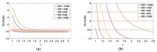
Figure 7.
The desired broadening factor under different ISRs. (a) The relationship between the broadening factor and the ISLR under different ISRs, original result; (b) local enlargement of (a).
Figure 8.
The broadening factor fitted curve.
Table 6.
The coefficients of different referenced values obtained from Figure 8.
Consequently, the proposed approach can be completely carried out to suppress RFI. First, the RFI identification after smoothing is used to obtain the interference bandwidth and carrier frequency. According to the measured ISR, Equation (21) and coefficients listed in Table 6, the referenced broadening factor for RFI band-stop filtering can be obtained, and then the RFI signals could be well mitigated. Finally, the removed range spectrum is recovered by the abovementioned RSIAA, and then the range spectrum is still consistent.
5. Results
In order to validate the proposed RFI suppression approach, simulation experiments on simulated targets and real SAR data are carried out in this section. Based on properties of the RFI signals [8,10], L band SAR is more easily effected by RFI signals, while simulation parameters are listed in Table 7. To demonstrate the advantages of the proposed approach, SAR images with RFI without the RSIAA after RFI mitigation and with the RSIAA after RFI mitigation are compared, and the flowchart of the following designed simulation experiments is shown in Figure 9.
Table 7.
Simulation parameters of the SAR data.
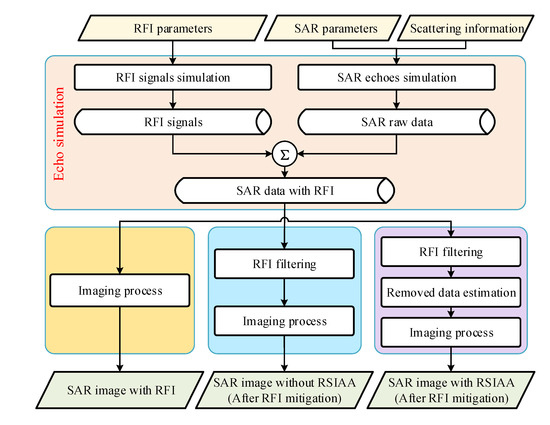
Figure 9.
Flowchart of the designed simulation experiments.
5.1. Simulation on Point Targets
One-dimensional (1D) simulation results of three designed points with the designed ISR of 5 dB are shown in Figure 10, and the RFI amplitude is significantly higher than the amplitude of SAR echoes in the frequency domain. According to coefficients listed in Table 6, the RFI signal is mitigated well by band-stop filtering with the broadening factor , as shown Figure 10b. Figure 10c shows that the removed spectrum of the desired echoes is recovered well by the RSIAA. Compared with the compression result without the RSIAA, the sidelobes are obviously suppressed, as shown in Figure 10d.
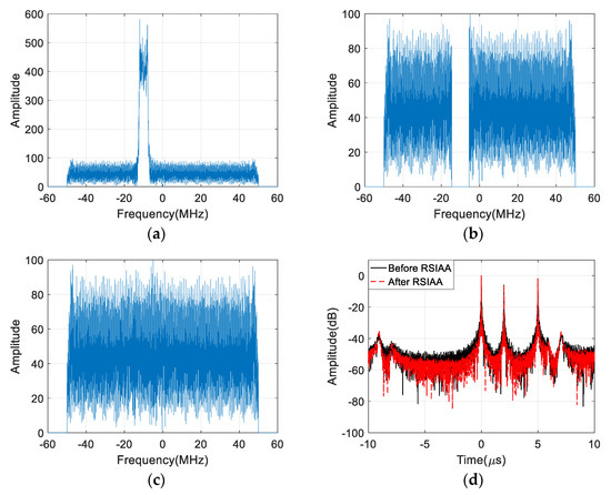
Figure 10.
1D Simulation results on point targets. (a) The spectrum with RFI; (b) after the band-stop filtering; (c) after the RSIAA; (d) comparisons of the pulse compression results.
To further evaluate the proposed approach, the 2D simulation experiments are designed, and they are shown in the flow chart of Figure 10, while simulation parameters are listed in Table 7. In Figure 11, the five point simulation results are shown. After RFI when the ISR is 10 dB, the frequency band is obviously interfered, as shown in Figure 11a, and in the imaging result exist some bright lines in the range direction, as shown in Figure 11b. Then, the RFI is removed by the band-stop filtering with the broadening factor , resulting in the discontinuous spectrum, as shown in Figure 11c, while the imaging quality of point targets is degraded in the range direction, as shown in Figure 11d. Fortunately, the removed spectrum is recovered well by the proposed approach in Figure 11e. Therefore, the five point targets are focused well, as shown in Figure 11f. In addition, contour plots of Point 1, 3 and 5 are demonstrated in Figure 11g–i, respectively. Meanwhile, the imaging performances of the five targets, including PLSR, ISLR and Res., are measured and listed in Table 8.
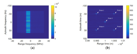
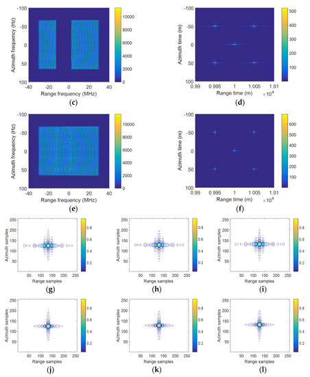
Figure 11.
2D simulation results on point targets. (a) The interfered 2D spectrum; (b) the imaging result with RFI; (c) the 2D spectrum after band-filtering; (d) the imaging result of (d); (e) the reconstructed spectrum; (f) the imaging result after the RSIAA; (g–i) contour plots of Point 1, 3 and 5 in (c); (j–l) contour plots of Point 1, 3 and 5 in (f).
Table 8.
The performance of five points.
5.2. Simulation of Distributed Scene
In order to further validate the proposed RFI suppression method, a focused SAR image of TerraSAR-X is used for simulation experiments and is obtained from the website [33]. RFI signals are intentionally added to this SAR image according to the simulation flow chart in Figure 10, and the parameters are listed in Table 7. With the ISR of 10 dB, the SAR image is completely contaminated by RFI, as shown in Figure 12a. The RFI signal is removed by the band-stop filtering operation with the broadening factor of 1.5, but the SAR image has an increased noisy background in Figure 12b due to artifacts and high sidelobes in the range direction caused by the discontinuous spectrum. After taking the RSIAA, artifacts and high sidelobes in the range direction are suppressed. A point target in the marked area A, as shown in Figure 12, is used to evaluate the effect of RFI mitigation and the image quality. From the comparison of focused images and contour plots of point targets in the marked area A, the band-stop filtering shows an effective RFI suppression effect but has a high sidelobe level, and the imaging quality is obviously improved after the RSIAA. Imaging performances of the point target in the marked area A both without and with the RSIAA are measured and summarized in Table 9. According to measured imaging performances in Table 9, the performance of the ISLR is obviously improved, and it also explains why the focused SAR image in Figure 12c is better than the image in Figure 12b.
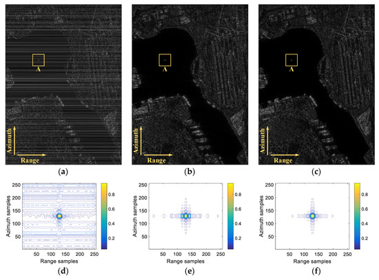
Figure 12.
Simulation results of the distributed scene. (a) The focused SAR image with RFI; (b) the focused SAR image without the RSIAA; (c) the focused SAR image with the RSIAA; (d–f) contour plots of the point target in the marked area of (a–c).
Table 9.
Measured imaging performances of the point target in the marked area A.
5.3. Results of Real SAR Data
5.3.1. Results of Gaofen-3 SAR Data
In this section, RFI signals are intentionally added to two sets of C band SAR real raw data of the Chinese Gaofen-3 (GF-3) satellite to further validate the proposed RFI suppression approach, and the bandwidth of the GF-3 SAR data is 100 MHz. The designed carrier frequency and bandwidth of the RFI signal are 5.42 GHz and 5 MHz, respectively, while the raw data of the RFI signal with different ISRs are simulated according to GF-3 SAR parameters. The original GF-3 SAR image has a size of 20,145 × 21,030 points, and marked area 1 and area 2 in Figure 13 are used to validate the proposed approach, as shown in Figure 14 and Figure 15 in the manuscript. The ISR in Figure 14 is 10 dB, while the ISR in Figure 15 is 15 dB. After adding the RFI signals to the GF-3 SAR data, the focused SAR images are fully polluted, as shown in Figure 14a and Figure 15a. The band-stop filtering is conducted to remove the RFI signal with the broadening factor of 1.5, and the SAR image quality is improved after the RSIAA, especially for marked area A in Figure 14c and marked area B in Figure 15c. Furthermore, the range profiles are compared and shown in Figure 14d and Figure 15d, and the artifacts and high sidelobes due to the removed spectrum are obviously suppressed by the RSIAA.
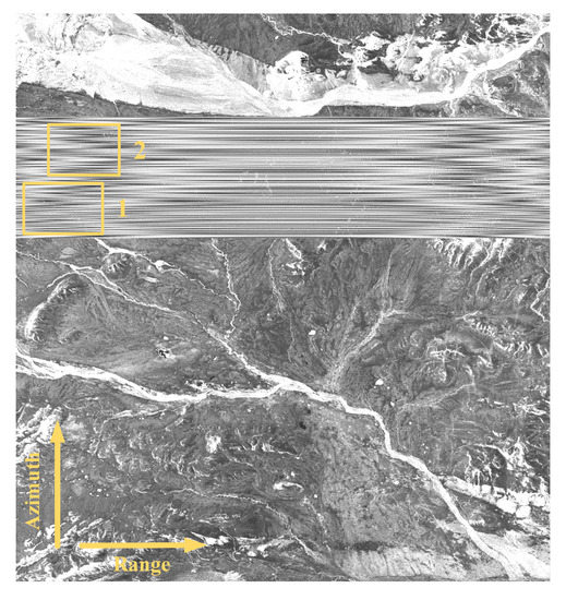
Figure 13.
The SAR original image of Gaofen-3 (GF-3) with RFI.
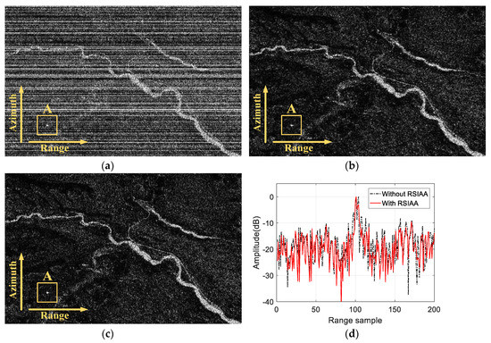
Figure 14.
Imaging results of the first set of GF-3 SAR data. (a) The SAR image with RFI; (b) the SAR image without the RSIAA; (c) the SAR image with the RSIAA; (d) range profiles of the target in area A.
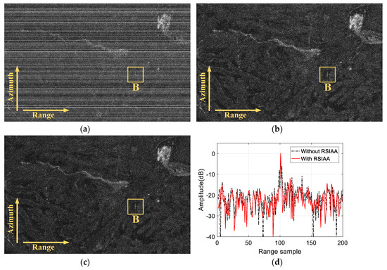
Figure 15.
Imaging results of the second set of GF-3 SAR data. (a) The SAR image with RFI; (b) the SAR image without the RSIAA; (c) the SAR image with the RSIAA; (d) range profiles of the target in area B.
5.3.2. Results of Sentinel-1 SAR Data
Similarly, RFI signals with the carrier frequency of 5.37 G and the bandwidth of 8 MHz are added to the two sets of C band SAR data of the Sentinel-1 satellite. The designed ISR in Figure 16 is 12 dB, and the one in Figure 17 is 15 dB. To demonstrate the image quality improvements in Figure 16c and Figure 17c, two strong point-like targets in marked area C of Figure 15 and marked area D of Figure 16 are tested, and their range profiles are plotted in Figure 16d and Figure 17d, respectively. According to the range profile comparison results without and with the RSIAA, the artifacts and high sidelobes due to the discontinuous range spectrum are obviously suppressed by the RSIAA.
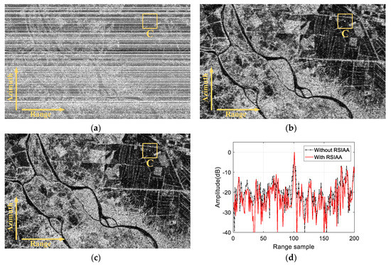
Figure 16.
Imaging results of the first set of Sentinel-1 SAR data. (a) The SAR image with RFI; (b) the SAR image without the RSIAA; (c) the SAR image with the RSIAA; (d) range profiles of the target in area C.
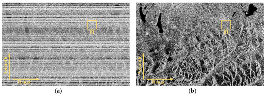
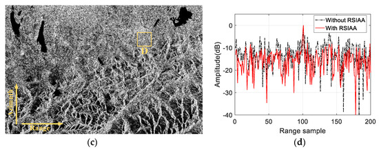
Figure 17.
Imaging results of the second set of Sentinel-1 SAR data. (a) The SAR image with RFI; (b) the SAR image without the RSIAA; (c) the SAR image with the RSIAA; (d) range profiles of the target in area D.
6. Discussion
In this paper, the proposed RFI suppression approach includes three important steps: RFI identification, band-stop filtering and the RSIAA. Compared with the parametric interference suppression approaches, the proposed method exploits the spectral characteristic to filter out RFI and reconstruct the useful spectrum in the frequency domain without any prior knowledge or precise model. However, the following points should be considered when the proposed approach is adopted to suppress RFI.
- (1)
- The smoothing process is added before RFI signal detection, which improved the RFI detection capacity, but a reasonable window size should be carefully designed according to characteristics of RFI signals. The narrow and weak RFI may be ignored with a large smoothing window, thus the smoothing operation is conducted step by step.
- (2)
- The broadening factor is proposed to mitigate the residual RFI that ensures the RSIAA accuracy. Based on simulated experiments, the selected broadening factor can be a little larger than the referenced value in practice, but one that is too large will consume more computational resources and time. Therefore, a compromise is needed between the accuracy and the computational complexity in practice.
- (3)
- The image quality improvement due to the removed spectrum recovery is related to the complexity of the imaged scene, similar to compressed sensing theory [34]. Furthermore, the larger iteration number brings higher estimation accuracy, but causes more serious computational consumption. Consequently, an appropriate number of iterations must be adopted to obtain the satisfactory accuracy and an affordable computation burden.
7. Conclusions
In this paper, a nonparametric interference suppression approach based on the RSIAA is proposed, which is combined with RFI identification and band-stop filtering. Since the small amount of residual RFI energy due to the Gibbs phenomenon in DFT will still affect the SAR image quality and decrease the accuracy of the RSIAA, a broadening factor, which is related to the ISR level and tolerance limits of the SAR image quality degradation, is introduced for range spectrum band-stop filtering. The major disadvantage of band-stop filtering for RFI mitigation is part of the effective range spectrum of the desired echoes is simultaneously removed with RFI signals. Compared with the bandwidth of the SAR system, the bandwidth of band-stop filtering is relatively limited, but it would still result in the increased sidelobes and artifacts in the range direction and obviously degrade the SAR image quality. Consequently, the iterative adaptive approach for removed spectrum estimation, which is named as the RSIAA, is used to reconstruct the removed spectrum of the desired echoes. The IAA filter size, the number of iterations and data volume of spectrum components for the RSIAA would affect the accuracy of the removed spectrum reconstruction, while more accurate spectrum estimation requires more effective data, computing resources and time. According the signal model of the RSIAA, the sparse imaged scene is more suitable for the proposed RFI suppression method due to being much less time-consuming. RFI signals are suppressed by the band-stop filtering for both the simulated raw data and the real SAR data, but the SAR image qualities in all cases are degraded due to the discontinuous range spectra. After the removed range spectra recovery by the RSIAA, the range sidelobe level of the simulated point target is suppressed by about 4dB, while the range sidelobe levels of the strong point-like target in GF-3 and Sentinel-1 SAR data are suppressed by about 3dB.
Author Contributions
All the authors made a contribution to this work. W.X. (Wei Xu) and W.X. (Weida Xing) proposed the idea and wrote the paper; C.F. conceived and designed the experiments; P.H. performed the experiments; W.T. and Z.G. revised the manuscript. All authors have read and agreed to the published version of the manuscript.
Funding
This research was supported in part by the Equipment Pre-research Field Foundation under Grant Nos. JZX7Y20190253040501, JZX7Y20190253041401 and JZX7Y20190253040901, in part by the National Natural Science Foundation of China under Grant Nos. 61761037, 61631011 and 61701264, in part by the Key Laboratory Foundation under Grant No. 6142216190209 and in part by the Natural Science Foundation of Inner Mongolia of China under Grant No. 2020ZD018.
Conflicts of Interest
The authors declare no conflict of interest.
References
- Curlander, J.C.; McDonough, R.N. Synthetic Aperture Radar: Systems and Signal Processing; John Wiley & Sons Ltd.: New York, NY, USA, 1991. [Google Scholar]
- Natsuaki, R.; Motohka, T.; Watanabe, M.; Shimada, M.; Suzuki, S. An autocorrelation-based radio frequency interference detection and removal method in azimuth-frequency domain for SAR Image. IEEE J. Sel. Top. Appl. Earth Obs. Remote Sens. 2017, 10, 5736–5751. [Google Scholar] [CrossRef]
- Wang, W.-Q.; Shao, H. Radar-to-Radar Interference Suppression for Distributed Radar Sensor Networks. Remote Sens. 2014, 6, 740–755. [Google Scholar] [CrossRef]
- Shen, W.; Qin, Z.; Lin, Z. A New Restoration Method for Radio Frequency Interference Effects on AMSR-2 over North America. Remote Sens. 2019, 11, 2917. [Google Scholar] [CrossRef]
- Shimada, M. L-band radio interferences observed by the jers-1 SAR and its global distribution. In Proceedings of the 2005 IEEE International Geoscience and Remote Sensing Symposium, Seoul, Korea, 25–29 July 2005; pp. 2752–2755. [Google Scholar]
- Paul, A.; Scott, H.; Charles, L. Observations and mitigation of RFI in ALOS PALSAR SAR data: Implications for the DESDynI mission. In Proceedings of the 2008 IEEE Radar Conference, Rome, Italy, 26–30 May 2008; pp. 1–6. [Google Scholar]
- Griffiths, H.; Cohen, L.; Watts, S.; Mokole, E.; Baker, C.; Wicks, M.; Blunt, S. Radar Spectrum Engineering and Management: Technical and Regulatory Issues. Proc. IEEE 2015, 103, 85–102. [Google Scholar] [CrossRef]
- Su, J.; Tao, H.; Tao, M.; Xie, J.; Wang, Y.; Wang, L. Time-Varying SAR Interference Suppression Based on Delay-Doppler Iterative Decomposition Algorithm. Remote Sens. 2018, 10, 1491. [Google Scholar] [CrossRef]
- Zhou, F.; Xing, M.; Bai, X.; Sun, G.; Bao, Z. Narrow-Band Interference Suppression for SAR Based on Complex Empirical Mode Decomposition. IEEE Geosci. Remote Sens. Lett. 2009, 6, 423–427. [Google Scholar] [CrossRef]
- Liu, Z.; Liao, G.; Yang, Z. Time Variant RFI Suppression for SAR Using Iterative Adaptive Approach. IEEE Geosci. Remote Sens. Lett. 2013, 10, 1424–1428. [Google Scholar] [CrossRef]
- Huang, X.; Liang, D. Gradual RELAX Algorithm for RFI Suppression in UWB-SAR. Electron. Lett. 1999, 35, 1916–1917. [Google Scholar] [CrossRef]
- Luo, X.; Ulander, L.M.; Askne, J.; Smith, G.; Frolind, P.O. RFI Suppression in Ultra-Wideband SAR Systems Using LMS Filters in Frequency Domain. Electron. Lett. 2001, 37, 241–243. [Google Scholar] [CrossRef]
- Miller, T.; Potter, L.; Mccorkle, J. RFI Suppression for Ultra Wideband Radar. IEEE Trans. Aerospace Electron. Syst. 1997, 33, 1142–1156. [Google Scholar] [CrossRef]
- Load, R.T.; Inggs, M.R. Efficient RFI Suppression in SAR Using LMS Adaptive Filter Integrated with Rang/Doppler Algorithm. Electron. Lett. 1999, 35, 629–630. [Google Scholar]
- Won, J.H.; Pany, T.; Eissfeller, B. Iterative Maximum Likelihood Estimators for High-Dynamic GNSS Signal Tracking. IEEE Trans. Aerosp. Electron. Syst. 2012, 48, 2875–2893. [Google Scholar] [CrossRef]
- Nguyen, L.; Soumekh, M. Suppression of Radio Frequency Interference (RFI) For Synchronous Impulse Reconstruction Ultra-Wideband Radar. Proc. SPIE 2005, 5808, 178–184. [Google Scholar]
- Yi, J.; Wan, X.; Cheng, F.; Gong, Z. Computationally Efficient RF Interference Suppression Method with Closed-Form Maximum Likelihood Estimator for HF Surface Wave Over-The-Horizon Radars. IEEE Trans. Geosci. Remote Sens. 2013, 51, 2361–2372. [Google Scholar] [CrossRef]
- Guo, Y.; Zhou, F.; Tao, M.; Sheng, M. A New Method for SAR Radio Frequency Interference Mitigation Based on Maximum a Posterior Estimation. In Proceedings of the 2017 32nd General Assembly and Scientific Symposium of the International Union of Radio Science, Montreal, QC, Canada, 19–26 August 2017; pp. 1–4. [Google Scholar]
- Ojowu, O.; Li, J. RFI Suppression for Synchronous Impulse Reconstruction UWB Radar Using RELAX. Int. J. Remote Sens. Appl. 2013, 3, 33–46. [Google Scholar]
- Bollian, T.; Osmanoglu, B.; Rincon, R.; Lee, S.-K.; Fatoyinbo, T. Adaptive Antenna Pattern Notching of Interference in Synthetic Aperture Radar Data Using Digital Beamforming. Remote Sens. 2019, 11, 1346. [Google Scholar] [CrossRef]
- Díez-García, R.; Camps, A. Impact of Signal Quantization on the Performance of RFI Mitigation Algorithms. Remote Sens. 2019, 11, 2023. [Google Scholar] [CrossRef]
- Zhou, F.; Wu, R.; Xing, M.; Bao, Z. Eigensubspace-Based Filtering with Application in Narrow-Band Interference Suppression for SAR. IEEE Geosci. Remote Sens. Lett. 2007, 4, 75–79. [Google Scholar] [CrossRef]
- Le, C.T.C.; Hensley, S.; Chapin, E. Removal of RFI in Wideband Radars. In Proceedings of the 2005 IEEE International Geoscience and Remote Sensing Symposium, Seattle, WA, USA, 6–10 July 1998. [Google Scholar]
- Tao, M.; Zhou, F.; Zhang, Z. Wideband Interference Mitigation in High-Resolution Airborne Synthetic Aperture Radar Data. IEEE Trans. Geosci. Remote Sens. 2016, 54, 74–87. [Google Scholar] [CrossRef]
- Liu, H.; Li, D. RFI Suppression Based on Sparse Frequency Estimation for SAR Imaging. IEEE Geosci. Remote Sens. Lett. 2016, 13, 63–67. [Google Scholar] [CrossRef]
- Stoica, P.; Li, J.; Ling, J. Missing Data Recovery Via a Nonparametric Iterative Adaptive Approach. IEEE Signal Process. Lett. 2009, 16, 241–244. [Google Scholar] [CrossRef]
- Stanković, L.; Orović, I.; Stanković, S.; Amin, M. Compressive Sensing Based Separation of Nonstationary and Stationary Signals Overlapping in Time-Frequency. IEEE Tran. Signal Process. 2013, 61, 4562–4572. [Google Scholar] [CrossRef]
- Fan, W.; Zhou, F.; Tao, M.; Bai, X.; Rong, P.; Yang, S.; Tian, T. Interference Mitigation for Synthetic Aperture Radar Based on Deep Residual Network. Remote Sens. 2019, 11, 1654. [Google Scholar] [CrossRef]
- Huang, Y.; Zhang, L.; Li, J.; Chen, Z.; Yang, X. Reweighted Tensor Factorization Method for SAR Narrowband and Wideband Interference Mitigation Using Smoothing Multiview Tensor Model. IEEE Trans. Geosci. Remote Sens. 2020, 58, 3298–3313. [Google Scholar] [CrossRef]
- Synthetic Aperture Radar-Imsar. Available online: https://www.imsar.com/portfolio-posts/synthetic-aperture-radar (accessed on 14 September 2020).
- Yardibi, T.; Li, J.; Stoica, P.; Xue, M.; Baggeroer, A.B. Source Localization and Sensing: A Nonparametric Iterative Adaptive Approach Based on Weighted Least Squares. IEEE Tran. Aerosp. Electron. Syst. 2010, 46, 425–443. [Google Scholar] [CrossRef]
- Wang, Y.; Li, J.; Stoica, P. Spectral Analysis of Signals, The Missing Data Case, 1st ed.; Morgan & Claypool: San Rafael, CA, USA, 2005. [Google Scholar]
- TerraSAR-X Satellites Geoimage. Available online: https://www.geoimage.com.au/satellite/TerraSar (accessed on 14 September 2020).
- Donoho, D.L. Compressed sensing. IEEE Trans. Inf. Theory 2006, 52, 1289–1306. [Google Scholar] [CrossRef]


Publisher’s Note: MDPI stays neutral with regard to jurisdictional claims in published maps and institutional affiliations. |
© 2020 by the authors. Licensee MDPI, Basel, Switzerland. This article is an open access article distributed under the terms and conditions of the Creative Commons Attribution (CC BY) license (http://creativecommons.org/licenses/by/4.0/).