Abstract
An increasing number of satellite platforms provide daily images of the Earth’s surface that can be used in quantitative monitoring applications. However, their cost and the need for specific processing software make such products not often suitable for rapid mapping and deformation tracking. Google Earth images have been used in a number of mapping applications and, due to their free and rapid accessibility, they have contributed to partially overcome this issue. However, their potential in Earth’s surface displacement tracking has not yet been explored. In this paper, that aspect is analyzed providing a specific procedure and related MATLAB™ code to derive displacement field maps using digital image correlation of successive Google Earth images. The suitability of the procedure and the potential of such images are demonstrated here through their application to two relevant case histories, namely the Slumgullion landslide in Colorado and the Miage debris-covered glacier in Italy. Result validation suggests the effectiveness of the proposed procedure in deriving Earth’s surface displacement data from Google Earth images.
1. Introduction
In the last decades, an increasing number of satellite platforms are persistently acquiring Earth observation data in the form of optical, multispectral, hyperspectral, and radar products (e.g., GeoEye, WorldView, Sentinel, Jilin, Radarsat, Envisat). Such products form a very important database for Earth surface control and mapping, offering a general medium to high resolution (0.3 to >50 m single-sided pixel dimension) and a revisiting time of a few days to a few weeks. The highest resolution products (<10 m single-sided pixel dimension) are often used for Earth’s surface deformation monitoring. Landslides, glaciers, earthquakes, and dune-field displacement tracking are examples of applications of satellite products that, covering small to large areas, have the potential to provide an exhaustive overview of the process [1,2,3,4].
Among the most effective techniques that can be used to monitor Earth’s surface displacement, the increasingly used interferometry technique called Differential Interferometric Synthetic Aperture Radar (DInSAR, [5,6]) has the potential to support low-rate deformation tracking applications and mapping [7,8,9,10]. Moreover, due to the characteristics of the sensors, it is able to work in all-weather and day and night conditions. However, this approach is not always suitable due to limitations related to the maximum detectable velocity [11] and potential high cost, especially in the context of high-resolution analyses (e.g., persistent scatterer approaches, [12,13]). This limitation has been partially overcome through the implementation of specific low-resolution approaches [14,15,16]. The use of optical images to track Earth’s surface displacement is a potential alternative to SAR interferometry that has no limitations in terms of maximum detectable velocity and has the potential to be used in a number of deformation scenarios [17,18,19,20,21]. Similar to SAR imagery, there are major limitations, where optical images are not suitable for fast mapping and fast process understanding, because of their relevant cost especially for very large areas and the time necessary to access the data.
In this perspective, the freely and immediately available Google Earth images have supported a number of studies, especially in the context of change detection and mapping application. For instance, the authors of [22] utilized Google Earth imagery to produce an inventory of rock glaciers in the central British Columbia Coast Mountains of Canada. Using a similar methodology, the researchers of [23] mapped 487 glaciers and their corresponding maximum LIA glacial advances in the central Tien Shan of China, analyzing the relationships between the magnitude of glacier changes and local topographic conditions. In [24], the authors demonstrated the suitability of Google Earth imagery to analyze channel width variability, as well as landslide and distributed fault characteristics. In [25], the researchers used Google Earth images to map landslides triggered by the 2008 M7.9 Wenchuan earthquake. In addition, the authors of [26] indicated that Google Earth images have a general 2D accuracy in positioning around 1 m, which confirms their suitability in deriving accurate ground measurements.
Although many studies have explored and demonstrated the suitability of Google Earth imagery in mapping applications and the ability of the platform in providing quantitative datasets about landslides and glaciers, the usefulness of such imagery in deriving deformational data has not yet been explored. On this basis, the suitability of Google Earth imagery for tracking Earth’s surface displacement is analyzed in this paper, presenting a dedicated implementation of the Kanade–Lucas–Tomasi (KLT) algorithm in a multi-step procedure (i.e., image pre-processing and subsequent displacement analysis, [27,28]) capable of providing displacement data in the form of displacement field maps and graphs. The presented procedure was coded in a MATLAB™ environment and should have the potential to be used in a number of applications including landslide and glacier kinematic analyses as well as fault deformation analysis. The suitability of the procedure is demonstrated here through its application to two relevant case histories, namely the Slumgullion landslide in southwestern Colorado, USA (Figure 1a; [29,30]), which is consistently moving since at least the last three centuries, and the Miage debris-covered glacier in Italy, which is subject to seasonal displacement (Figure 1b; [31]). A discussion and a validation of the results are presented using a comparison with available velocity data and considering the expected behavior of the landslide and glacier.
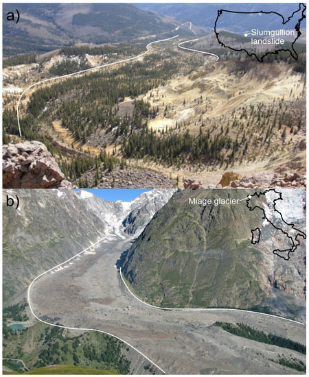
Figure 1.
(a) Slumgullion landslide as seen from the top of the head looking toward southwest. (b) Miage glacier as seen from the opposite flank of the Veny valley. Artworks indicate the approximate boundary of the moving landslide and glacier tongue.
2. Study Areas
2.1. Slumgullion Landslide
The Slumgullion landslide is located in the San Juan Mountains of southwestern Colorado, USA, and consists in a 3.9 km long, slow-persistently moving, active landslide associated with a larger and dormant landslide deposit (Figure 1a; [30,32]). The active landslide ranges in elevation from 2950 to 3650 m asl and the slope of the ground surface is of approximately 8°. Total landslide volume has been estimated as ~20 × 106 m3 and the average thickness is around 13 m [29]. The landslide has a typical flow-like surface morphology and therefore, although the movement occurs mainly by sliding along discrete basal and lateral slip surfaces, it has been described as an earthflow [29]. The Slumgullion landslide has been actively moving since at least 300 years ago. Landslide velocity ranges between approximately 0.15 and 7 m/year [30]. Higher velocities have been observed along the longitudinal center of the middle sector of the landslide and lower velocities have been observed at the head and the toe. Velocity variations in space materialize distinct kinematic elements bounded by deformational structures [30]. The landslide moves more slowly during winter when most precipitation falls as snow and faster during spring due to snowmelt and rainfall events [30]. The authors of [33] indicate that, over the next century, the landslide movement rate is expected to decrease due to a change in regional moisture balance conditions. This seems to be consistent with estimations completed by the authors of [16,34], indicating a maximum velocity from 4 to 4.4 m/year in the period 2011–2013.
2.2. Miage Debris-Covered Glacier
The Miage Glacier is in the eastern Alps along the southwestern side of Mont Blanc in the Veny valley of northern Italy (Figure 1b). It consists of a 6 km debris-covered glacier with a total surface of approximately 11 km2 [31]. The debris cover extends from an elevation of approximately 2400 m asl, downslope, toward the frontal lobes forming the lower end of the ablation tongue. Grain size of debris forming the glacier cover ranges from rock boulders to fine pebbles and sand. Debris cover thickness ranges between a few cm of the upper sector to 1.5 m of the lower sector and is consistently related to surface slope. Its presence is sustained by continuous rockfalls and rock avalanches [31] and its movement is consistently related to glacier-tongue seasonal displacement. The upper and middle sectors of the tongue move with an estimated average velocity of approximately 60 m/year [31,35]. In the lower sector of the ablation tongue, velocity decreases to an average of 45 m/year with further notable reduction toward the lower end of the glacier tongue. In this zone, velocity decreases to less than 4 m/year and reaches approximately 20 m/year next to the beginning of the southern lobe [31].
3. Materials and Methods
For estimating the displacement of both the medium and lower sectors of the active part of the Slumgullion landslide and the medium and lower sectors of the Miage debris-covered glacier, color Google Earth images saved as 4800 × 2674 jpeg files were used. Images depicting the active part of the Slumgullion landslide were acquired on 6 June 2013 and 14 October 2015. Images representative of the Miage glacier valley were acquired on 29 August 2009 and 28 May 2011. In both cases, following the master/slave logic of the digital image correlation technique, the first image was used as master and the second one as slave.
The procedure used for image selection, acquisition, and processing is reported in Figure 2. Prior to image selection, the study area (for each case study) was identified into a GIS environment and a rectangular polygon with a dimension of 2400 × 1337 m (H/L ratio ~ 0.55) was created and exported into a shp format. The dimension of the polygon was arbitrarily estimated considering the maximum available resolution of Google Earth images and the need for an acceptable final single-sided pixel dimension (in this case around 0.5 m). Corner coordinates of the polygon were exported in a separated text file for subsequent use in image rectification. Once imported into Google Earth, the polygon was used as reference for image selection. Specifically, after fitting the polygon to the screen by adjusting both image position and scale, acquisition dates of interest were selected, and the corresponding color images were acquired (Figure 3). In this case, acquisition dates were selected as a function of image sharpness. The images were saved with the reference polygon draped on them for subsequent processing. Specifically, after importing images into a GIS environment, they were digitally rectified considering four pairs of corner coordinates corresponding to the polygon vertex and affine method [36]. This procedure consists in the georeferentiation of the images through digital rectification, allowing the improvement of master and slave image co-registration. The error related to image rectification (i.e., co-registration) multiplied by 2 was considered as the accuracy of detected image feature position and was considered in displacement field map restitution. Once rectified, images were exported as geotiff selecting two different resolutions (i.e., pixel dimension). A first set (i.e., master and slave) was exported selecting full resolution (i.e., 0.5 m single-sided pixel dimension) and a second one (master image only) selecting the prospective resolution of the displacement grid used for final displacement mapping (i.e., 50 m single-sided pixel dimension). The first, high-resolution, set was directly used in tracking analysis. The second set was simply used for subsequent mapping, and its resolution (50 m was selected for this analysis) can be arbitrarily selected as a function of specific needs.
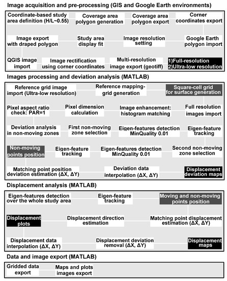
Figure 2.
Flow chart showing the logic of the algorithm used for digital image correlation of Google Earth imagery. White boxes indicate steps for each major phase of the analysis. Grey boxes indicate intermediate products used for subsequent steps. Black boxes indicate final products of each major phase of the analysis.
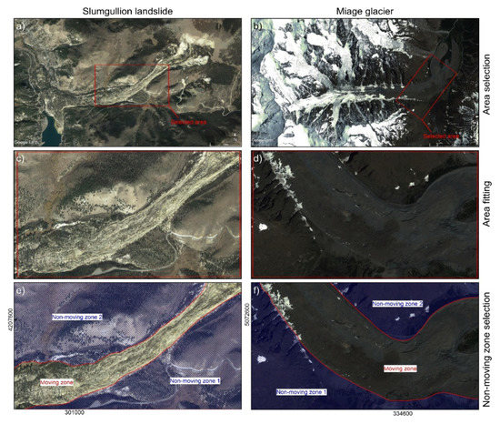
Figure 3.
Selection scheme of Google Earth images and moving and non-moving zone identification: (a,b) study areas identification; (c,d) image fitting; (e,f) moving and non-moving zone identification. Acquisition dates are June 6, 2013 for the images depicted in (a,c,e) and 29 August 2009 for the images depicted in (b,d,f). Map data 2020 © Maxar Technologies.
Once generated, images were processed using a specifically developed two-step procedure, coded in MATLAB™ (R2019b, © 1994–2020 The MathWorks, Inc., Natickc, MA, USA) (see Figure 2). Such a procedure, based on an eigen feature identification approach (i.e., corner points; [37]), uses the Kanade–Lucas–Tomasi (KLT) feature-tracking algorithm [27,28] which is applied to greyscale-rectified images to estimate the displacement of corner points in the time interval between successive image acquisitions. The KLT method allows to obtain displacement in the form of tracked feature displacement vectors, displacement components, 2D displacement distribution graphs, and displacement field maps. Algorithm parameterization was consistently completed using a trial and error procedure aimed at maximizing the number of trackable corner points and reducing the displacement estimation error. Minimum accepted quality of corners in the image, in the form of a fraction of the maximum corner metric value, was considered equal to 0.01. A maximum forward-backward bidirectional error threshold of 0.05 pixels was adopted to eliminate points that could not be reliably tracked. Additionally, since the KLT-based point tracker uses image pyramids, where each level is reduced in resolution by a factor of two compared to the previous level, and considering that the number of pyramid levels is related to the magnitude of the displacement to handle, seven pyramid levels were considered for the analysis.
In the first step (i.e., Image acquisition and pre-processing and Image processing and deviation analysis of Figure 2), the procedure accounts for the (i) preparation of a reference mapping grid through single ultra-low-resolution image (ULRis; i.e., 50 m single-sided pixel dimension), (ii) estimation of the full-resolution images’ pixel dimension, and (iii) definition of the displacement deviation (i.e., local error) through a controlled displacement analysis in known non-moving zones (see Figure 3). The reference mapping grid (i) is derived from the ULRis by emulating the image grid through vector meshing. Pixel dimension (ii) is consistently estimated from image–pixel coordinates and is stored in a specific variable that forms the basis for subsequent displacement estimation. Non-moving zones (iii) are selected by the user, creating a mask through the roipoly interactive tool implemented in MATLAB™. The code can be arranged with a selectable number of non-moving zones. In this case, since both image sets are characterized by a central moving zone, because of the presence of landslide and glacier, the code is arranged with two subsequent steps of non-moving zone identification. Once identified, the non-moving zone masks are used to support displacement analysis for local deviation estimation. This deviation is related to change in scale due to the potential presence of reliefs and image distortion that has not been successfully corrected by digital image rectification. Deviation estimation is completed using the corner point tracking approach described above and provides both X and Y components of deviation in the form of distribution graphs and raster maps. Such maps, derived by the spatial interpolation of data over the reference mapping grid, form the basis for the deviation compensation processing. Data interpolation is consistently completed using the natural neighbor method [38].
In the second step (i.e., Displacement analysis of Figure 2), the displacement analysis is completed without mask constraints, so that is extended to the whole study area depicted in the images. The KLT algorithm tracks identified corner points providing X and Y coordinates in the master and slave images. Such coordinates form the basis for displacement component estimation. Once estimated, displacement components are used to derive the displacement module and its direction through simple geometrical relations. The code provides a distribution graph of displacement. Subsequently, displacement components estimated at specific positions are used to derive X and Y displacement rasters through the spatial interpolation of data over the reference mapping grid. Such rasters are used to derive the displacement field map. Before deriving the displacement field map, X and Y component deviation rasters are subtracted from the X and Y displacement raster to remove the error related to residual image distortion. The final displacement field map shows the displacement distribution across the selected study area following a Lagrangian description scheme.
Once the displacement field is obtained, this is validated using a comparison with available local velocity data and considering the expected earthflow and glacier spatial kinematics [16,30,39,40,41].
4. Results
4.1. Slumgullion Landslide
The analysis indicates that the middle and lower sectors of the active part of the Slumgullion landslide consistently moved between 6 June 2013 and 14 October 2015 (860 days). A total of 7069 eigen features were successfully identified and tracked. Their distribution is shown in Figure 4a. As observed, the density of recognized features in the moving zone is much higher than in the non-moving zone and no outliers (displacement vectors related to inconsistently tracked objects) are visually recognizable. Image rectification, completed using the coordinates of image corners, indicates a rectification RMSE of ~1 m.
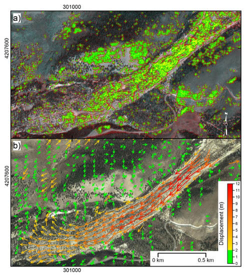
Figure 4.
Slumgullion landslide and surrounding slopes. (a) Eigen features identified and tracked within the study area. Centroid of red symbols indicates feature position in the master image (i.e., 6 June 2013), while green crosses indicate feature position in the slave image (i.e., 14 October 2015). (b) Displacement field map derived by eigen-feature tracking after deviation correction. UTM coordinates are shown at figure edges. Map data 2020 © Maxar Technologies.
Deviation analysis, conducted considering the NW and SE non-moving zones separated by the moving landslide, indicates for the X and Y displacement components a deviation ranging between −4 and +5 m, and −7 and +1 m, respectively (Figure 5a). The modes of distributions are, in both cases, at −1 m. X and Y deviation spatial distribution is reported in Figure 6a,b. Displacement component distribution as well as resultant 2D displacement are reported in the graph of Figure 5b, and displacement distribution is reported in the displacement field map of Figure 4b. As indicated in the graph, overall, a displacement ranging from −11 to + 5 m was registered along the X-axis of the image, while a displacement ranging from −7 to + 9 m was registered along the Y-axis. 2D resultant displacement ranges between 1 and 12.2 m. Considering the accuracy of positioning estimated as the RMSE multiplied by 2, that in this case is estimated as 2 m, 2D resultant displacement ranges between 0 and 10.2 to 14.2 m (i.e., 12.2 ± 2 m) for a maximum velocity ranging between ~4 and ~6 m/year.
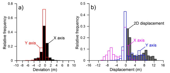
Figure 5.
Slumgullion landslide and surrounding slopes. (a) Distribution of deviation in displacement estimation as derived by feature tracking in non-moving zones. (b) Distribution of displacement components and 2D total displacement as estimated by feature tracking within both the moving and non-moving zones.
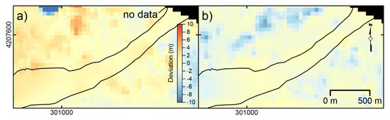
Figure 6.
Slumgullion landslide and surrounding slopes. (a) Distribution of deviation in displacement along the X-axis. (b) Distribution of deviation in displacement along the Y-axis. UTM coordinates are shown at figure edges. Black lines indicate moving area boundary.
4.2. Miage Debris-Covered Glacier
The analysis indicates that the middle and lower sectors of the Miage debris-covered glacier consistently moved between 29 August 2009 and 28 May 2011 (637 days). A total of 19,067 eigen features were successfully identified and tracked. Their distribution is shown in Figure 7a. As observed, the density of recognized feature in the moving zone is much higher than in the non-moving zone, although it is not fully covered. No outliers (displacement vectors related to inconsistently tracked objects) are visually recognizable. Image rectification, completed using the coordinates of image corners, indicates a rectification RMSE of ~1.5 m.
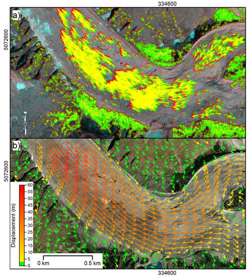
Figure 7.
Miage debris-covered glacier and surrounding slopes. (a) Eigen features identified and tracked within the study area. Centroid of red symbols indicates feature position in the master image (i.e., 29 August 2009), while green symbols indicate feature position in the slave image (i.e., 28 May 2011). (b) Displacement field map derived by eigen-feature tracking after deviation correction. UTM coordinates are shown at figure edges. Map data 2020 © Maxar Technologies.
Deviation analysis, conducted considering the NW and SE non-moving zones separated by the moving glacier, indicates for X and Y displacement components a deviation ranging between −5 and +8 m, and −5 and +10 m, respectively (Figure 8a). The modes of distributions are at +2 and +4 m, respectively. X and Y deviation spatial distribution is reported in Figure 9a,b. Displacement component distribution as well as resultant 2D displacement are reported in the graph of Figure 8b, and displacement distribution is reported in the displacement field map of Figure 7b. As indicated in the graph, overall, a displacement ranging from −6 to +34 m was registered along the X-axis of the image, while a displacement ranging from −20 to + 43 m was registered along the Y-axis. 2D resultant displacement ranges between 0.3 and 53 m. Considering the accuracy of positioning estimated as the RMSE multiplied by 2, that in this case is estimated as 3 m, 2D resultant displacement ranges between 0 and 59 m for a maximum velocity of ~33 m/year.
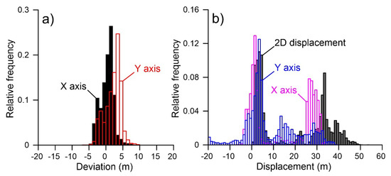
Figure 8.
Miage debris-covered glacier and surrounding slopes. (a) Distribution of deviation in displacement estimation as derived by feature tracking in non-moving zones. (b) Distribution of displacement components and 2D total displacement as estimated by feature tracking within both the moving and non-moving zones.
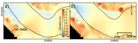
Figure 9.
Miage debris-covered glacier and surrounding slopes. (a) Distribution of deviation in displacement along the X-axis. (b) Distribution of deviation in displacement along the Y-axis. UTM coordinates are shown at figure edges. Black lines indicate moving area boundary.
5. Discussion and Validation
The growing archives of satellite optical remote sensing images and the advent of digital image correlation algorithms offer great potential for the detection and monitoring of landslides and glaciers [18,42,43,44]. In [18], the authors showed the use of Pléiades panchromatic images for the analysis of a landslide located in the South French Alps. They proposed the use of a multiple pairwise image correlation (MPIC) technique (to obtain horizontal displacement fields) and different multi-temporal indicators for a more accurate detection and quantification of surface deformations. Diversely from the research presented in [18], which aimed to improve the accuracy of image correlation techniques, the authors of [43] implemented a fuzzy Hough transform to analyze the GoLIVE dataset (https://nsidc.org/data/golive) with the goal of measuring seasonal velocity changes in glaciers, enhancing the extraction of the timing and location of ice flow events. A quantitative assessment of digital image correlation methods has been recently presented by the authors of [42], whose work demonstrated that all algorithms are capable of quantifying slope instability displacements, with average errors ranging from 8% to 12% of the observed maximum displacement.
In light of these elements of evidence, it is clear that image correlation techniques represent a powerful tool in the study of landslide and glacier deformation. However, the cost of the availability of satellite imagery still represents one of the main limitations of these techniques. In this context, the purpose of this research was to present a new low-cost and easily accessible method to perform image correlation types of studies, based on the use of freely available Google Earth imagery. The two case studies used as test sites were the Slumgullion landslide and the Miage debris-covered glacier. Results of the analysis indicate that both the Slumgullion landslide and the Miage debris-covered glacier actively moved in the reference period. This is consistent with previous analyses indicating that, in both cases, long-term movement has been observed and is expected for the near future [30,31]. In both cases, a typical displacement field for both flow-type landslide and glacier was observed.
The Slumgullion landslide moved with a maximum velocity, registered at the upper part of its middle sector, slightly below the landslide neck, around 5 m/year. The minimum velocity was registered at the toe with a rate around 1 m/year. These velocities are consistent with those calculated by the authors of [34] and predicted by the authors of [33]. Conversely, they appear to be much lower than those predicted by the authors of [30] for the period 1998–2002. This is consistent with the long-term prediction of the displacement rate completed by the authors of [33]. The displacement field of Figure 4b depicts a typical condition for this kind of landslide with velocity variations related to the width of the landslide corridor and to the distance from the toe. Specifically, as the width of the landslide corridor decreases, velocity increase and vice versa [40]. In addition, the proposed coded procedure seems to be able to recognize (lateral) spreading occurring at the toe of the slide and velocity reduction at cross-section edges.
The Miage glacier moved with a maximum velocity of 33 m/year between August 2009 and May 2011. This velocity was registered within the upper part of the lower sector of the ablation tongue where an average velocity of 45 m/year was registered by the authors of [31] between 1975 and 1991 (Figure 7b). This difference may be related to the ongoing reduction of glacier velocity connected to a deficit in mass balance induced by global warming, commonly observed in the Alpine region of Switzerland, France, and Italy [45,46,47]. A similar difference was also observable next to the beginning of the southern lobe where a velocity of 12 m/year was estimated.
In both cases, local inconsistent displacement vectors are present. Although they are mostly located along image edges, which are the most critical parts of images in object tracking perspective (see Figure 6a,b or Figure 9a,b), several occurrences can be recognized within both study regions. Those located along the edges of the images can be interpreted as local artefacts or false positives connected to the lack of an efficient tracking of non-moving points for generalized distortion compensation. Conversely, those located within the study areas may be representative of local error connected to the interpolation method. In addition, they can be considered as the indication of an erroneous interpretation of those areas as non-moving zones. This underlines a potential limit of the proposed procedure indicating that, in the absence of a detailed knowledge of the study area, results from the analysis have to be carefully interpreted and validated.
6. Conclusions
The analysis indicates that the proposed procedure and related MATLAB™ code are able to provide quantitative displacement data, in the form of displacement field maps and graphs, from the digital image correlation of Google Earth images. Such images require a specific acquisition scheme and need to be pre-processed to improve image co-registration and reduce internal distortion related to local-scale variation. The application to the Slumgullion landslide in Colorado (USA) and the Miage debris-covered glacier in Italy confirmed the potential of the procedure to derive a consistent estimation of displacement distribution and, at the same time, underlines its potential limit related to the knowledge of the study area as a pre-requisite needed to support result interpretation, especially in the absence of further quantitative data. This particular aspect, connected to the need of tracking displacement in a non-moving zone, is related to the need of reducing internal image deformation that may compromise displacement estimation over the whole area of interest.
Author Contributions
Conceptualization, L.G. and D.D.M.; methodology, L.G., D.D.M., and D.C.; software, L.G.; validation, M.F. and D.C.; formal analysis, L.G. and D.D.M.; investigation, D.C.; data curation, L.G.; writing—original draft preparation, L.G. and D.D.M.; writing—review and editing, M.F. and D.C.; supervision, M.F.; project administration, D.C. All authors have read and agreed to the published version of the manuscript.
Funding
This research received no external funding.
Acknowledgments
We thank Tom G. Farr and two anonymous reviewers for their constructive reviews of the paper. The code used for deriving the displacement data and the displacement field map is available upon request to Luigi Guerriero (luigi.guerriero2@unina.it).
Conflicts of Interest
The authors declare no conflict of interest.
References
- Solari, L.; Del Soldato, M.; Raspini, F.; Barra, A.; Bianchini, S.; Confuorto, P.; Casagli, N.; Crosetto, M. Review of Satellite Interferometry for Landslide Detection in Italy. Remote Sens. 2020, 12, 1351. [Google Scholar] [CrossRef]
- Di Martire, D.; Novellino, A.; Ramondini, M.; Calcaterra, D. A-Differential Synthetic Aperture Radar Interferometry analysis of a Deep Seated Gravitational Slope Deformation occurring at Bisaccia (Italy). Sci. Total Environ. 2016, 550, 556–573. [Google Scholar] [CrossRef] [PubMed]
- Herman, F.; Beyssac, O.; Brughelli, M.; Lane, S.N.; Leprince, S.; Adatte, T.; Lin, J.Y.Y.; Avouac, J.P.; Cox, S.C. Erosion by an Alpine glacier. Science 2015, 350, 193–195. [Google Scholar] [CrossRef] [PubMed]
- Vermeesch, P.; Leprince, S. A 45-year time series of dune mobility indicating constant windiness over the central Sahara. Geophys. Res. Lett. 2012, 39. [Google Scholar] [CrossRef]
- Gabriel, A.K.; Goldstein, R.M.; Zebker, H.A. Mapping small elevation changes over large areas: Differential interferometry. J. Geophys. Res. 1989, 94, 9183–9191. [Google Scholar] [CrossRef]
- Franceschetti, G.; Migliaccio, M.; Riccio, D.; Schirinzi, G. SARAS: A synthetic aperture radar (SAR) raw signal simulator. IEEE Trans. Geosci. Remote Sens. 1992, 30, 110–123. [Google Scholar] [CrossRef]
- Wasowski, J.; Bovenga, F. Investigating landslides and unstable slopes with satellite Multi Temporal Interferometry: Current issues and future perspectives. Eng. Geol. 2014, 174, 103–138. [Google Scholar] [CrossRef]
- Novellino, A.; Cigna, F.; Sowter, A.; Syafiudin, M.F.; Di Martire, D.; Ramondini, M.; Calcaterra, D. Intermittent small baseline subset (ISBAS) InSAR analysis to monitor landslides in Costa della Gaveta, Southern Italy. In IEEE International Geoscience and Remote Sensing Symposium, IGARSS; IEEE: Milan, Italy, 2015; pp. 3536–3539. [Google Scholar]
- Guerriero, L.; Confuorto, P.; Calcaterra, D.; Guadagno, F.M.; Revellino, P.; Di Martire, D. PS-driven inventory of town-damaging landslides in the Benevento, Avellino and Salerno Provinces, southern Italy. J. Maps 2019, 15, 619–625. [Google Scholar] [CrossRef]
- Ammirati, L.; Mondillo, N.; Rodas, R.A.; Sellers, C.; Di Martire, D. Monitoring Land Surface Deformation Associated with Gold Artisanal Mining in the Zaruma City (Ecuador). Remote Sens. 2020, 12, 2135. [Google Scholar] [CrossRef]
- Colesanti, C.; Ferretti, A.; Novali, F.; Prati, C.; Rocca, F. Sar monitoring of progressive and seasonal ground deformation using the permanent scatterers technique. IEEE Trans. Geosci. Remote Sens. 2003, 41, 1685–1701. [Google Scholar] [CrossRef]
- Ferretti, A.; Prati, C.; Rocca, F. Permanent scatterers in SAR interferometry. IEEE Trans. Geosci. Remote 2001, 39, 8–20. [Google Scholar] [CrossRef]
- Costantini, M.; Falco, S.; Malvarosa, F.; Minati, F. A new method for identification and analysis of persistent scatterers in series of SAR images. In Proceedings of the International Geoscience and Remote Sensing Symposium. (IGARSS), Boston, MA, USA, 7–11 July 2008; pp. 449–452. [Google Scholar]
- Michel, R.; Avouac, J.P.; Taboury, J. Measuring ground displacements from SAR amplitude images: Application to the landers earthquake. Geophys. Res. Lett. 1999, 26, 875–878. [Google Scholar] [CrossRef]
- Singleton, A.; Li, Z.; Hoey, T.; Muller, J.-P. Evaluating sub-pixel offset techniques as an alternative to D-InSAR for monitoring episodic landslide movements in vegetated terrain. Remote Sens. Environ. 2014, 147, 133–144. [Google Scholar] [CrossRef]
- Amitrano, D.; Giuda, R.; Dell’Aglio, D.; Di Martino, G.; Di Martire, D.; Iodice, A.; Costantini, M.; Malvarosa, F.; Minati, F. Long-Term Satellite Monitoring of the Slumgullion Landslide Using Space-Borne Synthetic Aperture Radar Sub-Pixel Offset Tracking. Remote Sens. 2019, 11, 369. [Google Scholar] [CrossRef]
- Mazzanti, P.; Caporossi, P.; Muzi, R. Sliding Time Master Digital Image Correlation Analyses of CubeSat Images for landslide Monitoring: The Rattlesnake Hills Landslide (USA). Remote Sens. 2020, 12, 592. [Google Scholar] [CrossRef]
- Stumpf, A.; Malet, J.P.; Delacourt, C. Correlation of satellite image time-series for the detection and monitoring of slow-moving landslides. Remote. Sens. Environ. 2017, 189, 40–55. [Google Scholar] [CrossRef]
- Kaab, A.; Altena, B.; Mascaro, J. Coseismic displacements of the 14 November 2016 Mw 7.8 Kaikoura, New Zealand, earthquake using the Planet optical cubesat constellation. Nat. Hazards Earth Syst. Sci. 2017, 17, 627–639. [Google Scholar] [CrossRef]
- Hollingsworth, J.; Leprince, S.; Ayoub, F.; Avouac, J.P. Deformation during the 1975-1984 Krafla rifting crisis, NE Iceland, measured from historical optical imagery. J. Geophys. Res. Solid Earth 2012, 117. [Google Scholar] [CrossRef]
- Herman, F.; Anderson, B.; Leprince, S. Mountain glacier velocity variation during a retreat advance cycle quantified using sub pixel analysis of ASTER images. J. Glaciol. 2011, 57, 197–207. [Google Scholar] [CrossRef]
- Charbonneau, A.A.; Smith, D.J. An inventory of rock glaciers in the Central British Columbia Coast Mountains, Canada, from high resolution Google Earth imagery. Arct. Antarct. Alp. Res. 2018, 50, e1489026. [Google Scholar] [CrossRef]
- Li, Y.; Li, Y. Topographic and geometric controls on glacier changes in the central Tien Shan, China, since the Little Ice Age. Ann. Glaciol. 2014, 55, 177–186. [Google Scholar] [CrossRef]
- Fisher, G.B.; Amos, C.B.; Bookhagen, B.; Burbank, D.W.; Godard, V. Channel Widths, Landslides, Faults, and Beyond: The New World Order of High Spatial Resolution Google Earth Imagery in the Study of Earth Surface Processes. In Google Earth and Virtual Visualizations in Geoscience Education and Research; Whitmeyer, S.J., Bailey, J.E., De Paor, D.G., Ornduff, T., Eds.; The Geological Society of America: Boulder, CO, USA, 2012; Volume 492, pp. 1–22. [Google Scholar] [CrossRef][Green Version]
- Sato, H.P.; Harp, E.L. Interpretation of earthquake-induced landslides triggered by the 12 May 2008, M7.9 Wenchuan earthquake in the Beichuan area, Sichuan Province, China using satellite imagery and Google Earth. Landslides 2009, 6, 153–159. [Google Scholar] [CrossRef]
- Pulighe, G.; Baiocchi, V.; Lupia, F. Horizontal accuracy assessment of very high resolution Google Earth images in the city of Rome, Italy. Int. J. Digit. Earth 2016, 9, 342–362. [Google Scholar] [CrossRef]
- Lucas, B.D.; Kanade, T. An Iterative Image Registration Technique with an Application to Stereo Vision. In Proceedings of the 7th International Joint Conference on Artificial Intelligence, Vancouver, BC, Canada, 24–28 August 1981; pp. 674–679. [Google Scholar]
- Tomasi, C.; Kanade, T. Detection and Tracking of Point Features. In Computer Science Department; Carnegie Mellon University: Pittsburgh, PA, USA, 1991. [Google Scholar]
- Parise, M.; Guzzi, R. Volume and Shape of the Active and Inactive Parts of the Slumgullion Landslide, Hinsdale County, Colorado; U.S. Geological Survey Open-File Report 92-216; U.S. Geological Survey: Reston, VA, USA, 1992; p. 29.
- Coe, J.A.; Ellis, W.L.; Godt, J.W.; Savage, W.Z.; Savage, J.E.; Michael, J.A.; Kibler, J.D.; Powers, P.S.; Lidke, D.J.; Debray, S. Seasonal movement of the Slumgullion landslide determined from Global Positioning System surveys and field instrumentation, July 1998–March 2002. Eng. Geol. 2003, 68, 67–101. [Google Scholar] [CrossRef]
- Diolaiuti, G.; Kirkbride, M.P.; Smiraglia, C.; Benn, D.I.; D’Agata, C.; Nicholson, L. Calving processes and lake evolution at Miage Glacier (Mont Blanc, Italian Alps). Ann. Glaciol. 2005, 40, 207–214. [Google Scholar] [CrossRef][Green Version]
- Crandell, D.R.; Varnes, D.J. Slumgullion earthflow and earth slide near Lake City. Colorado. Geol. Soc. Am. Bull. 1960, 71, 1846. [Google Scholar]
- Coe, J. Regional moisture balance control of landslide motion: Implication for landslide forecasting in a changing climate. Geology 2012, 40, 323–326. [Google Scholar] [CrossRef]
- Wang, C.; Cai, J.; Li, Z.; Mao, X.; Feng, G.; Wang, Q. Kinematic Parameter Inversion of the Slumgullion Landslide Using the Time Series Offset Tracking Method with UAVSAR Data. J. Geophys. Res. Solid Earth 2018, 123, 8110–8124. [Google Scholar] [CrossRef]
- Deline, P. Etude geomorphologique des interactions entre ecroulements rocheux et glaciers dans la haute montagne alpine: Le versant sud-est du Massif du Mont Blanc (Vallee d’Aoste, Italie). Ph.D. Thesis, Universite de Savoie, Chambery, France, 2002. [Google Scholar]
- Berger, M. Geometry I; Springer: Berlin, Germany, 1987; ISBN 3-540-11658-3. [Google Scholar]
- Shi, J.; Tomasi, C. Good Features to Track. In Proceedings of the IEEE Conference on Computer Vision and Pattern Recognition, Seattle, WA, USA, 21–23 June 1994; pp. 593–600. [Google Scholar]
- Sibson, R. A brief description of natural neighbor interpolation (Chapter 2). In Interpreting Multivariate Data; Barnett, V., Ed.; John Wiley: Chichester, England, 1981; pp. 21–36. [Google Scholar]
- Hooke, R. The velocity field in a glacier. In Principles of Glacier Mechanics; Cambridge University Press: Cambridge, UK, 2019; pp. 81–114. [Google Scholar]
- Guerriero, L.; Bertello, L.; Cardozo, N.; Berti, M.; Grelle, G.; Revellino, P. Unsteady sediment discharge in earth flows: A case study from the Mount Pizzuto earth flow, southern Italy. Geomorphology 2017, 295, 260–284. [Google Scholar] [CrossRef]
- Shangguan, D.; Liu, S.; Ding, Y.; Gou, W.; Xu, B.; Xu, J.; Jiang, Z. Characterizing the May 2015 Karayaylak Glacier surge in the eastern Pamir Plateau using remote sensing. J. Glaciol. 2016, 62, 944–953. [Google Scholar] [CrossRef]
- Bickel, V.T.; Manconi, A.; Amann, F. Quantitative Assessment of Digital Image Correlation Methods to Detect and Monitor Surface Displacements of Large Slope Instabilities. Remote Sens. 2018, 10, 865. [Google Scholar] [CrossRef]
- Altena, B.; Scambos, T.; Fahnestock, M.; Kääb, A. Extracting recent short-term glacier velocity evolution over southern Alaska and the Yukon from a large collection of Landsat data. Cryosphere 2019, 13, 795–814. [Google Scholar] [CrossRef]
- Bontemps, N.; Lacroix, P.; Doin, M.P. Inversion of deformation fields time-series from optical images, and application to the long term kinematics of slow-moving landslides in Peru. Remote Sens. Environ. 2018, 210, 144–158. [Google Scholar] [CrossRef]
- Huss, M.; Dhulst, L.; Bauder, A. New long-term mass-balance series for the Swiss Alps. J. Glaciol. 2015, 61, 551–562. [Google Scholar] [CrossRef]
- Gerbaux, M.; Genthon, C.; Etchevers, P.; Vincent, C.; Dedieu, J. Surface mass balance of glaciers in the French Alps: Distributed modeling and sensitivity to climate change. J. Glaciol. 2005, 51, 561–572. [Google Scholar] [CrossRef]
- Catasta, G.; Smiraglia, C. The mass balance of a cirque glacier in the Italian Alps (Ghiacciaio Della Sforzellina, Ortles–Cevedale Group). J. Glaciol. 1993, 39, 87–90. [Google Scholar] [CrossRef][Green Version]


Publisher’s Note: MDPI stays neutral with regard to jurisdictional claims in published maps and institutional affiliations. |
© 2020 by the authors. Licensee MDPI, Basel, Switzerland. This article is an open access article distributed under the terms and conditions of the Creative Commons Attribution (CC BY) license (http://creativecommons.org/licenses/by/4.0/).