Analysis of the Suitability of High-Resolution DEM Obtained Using ALS and UAS (SfM) for the Identification of Changes and Monitoring the Development of Selected Geohazards in the Alpine Environment—A Case Study in High Tatras, Slovakia

Abstract

The current trend in the use of remote sensing technologies is their use as a tool for monitoring hard-to-reach areas, objects or phenomena in the alpine environment. Remote sensing technology is also effectively used to monitor geohazards and the development of human-made changes in the country. Research presented in this study demonstrates the results for the usability of the publicly available national digital elevation model DEM 5.0 obtained by utilizing the airborne laser scanning (ALS) survey to monitor the development of erosion, morphological changes of talus cones, or the dynamics of movement of rock blocks between stages of measurement in the alpine environment of the High Tatras mountains. The reference methods for this study are the terrestrial laser scanning (TLS) and structure-from-motion (SfM) photogrammetric approach using unmanned aerial systems (UASs). By comparing the created DEMs, the ALS point cloud’s accuracy on mostly rocky areas of different sizes was verified. The results show that the standard deviation of the ALS point cloud ranges from 19 to 46 mm depending on the area’s size and characteristics. The maximum difference ranges from 100 to 741 mm. The value of systematic displacement of data obtained by different technologies ranges from 1 to 29 mm. This research confirms the suitability of the ALS method with its advantages and limits for the detection of movement of rock blocks or change of position of any natural or anthropogenic objects with a size from approximately 1 m².

1. Introduction

The development of mass data collection using aerial technologies [1,2] allowed one to document terrain changes and the development of geohazards in the alpine environment in a more accessible, more efficient, and more accurate way. Currently, unmanned aerial systems (UASs) utilize either digital image data (the structure from motion photogrammetric method), or small LiDARs (light detection and ranging). Another option is to use a laser scanner mounted on an aircraft. However, there are high acquisition costs, especially for the operation of the aircraft [3]. In many countries, for example, Czech Republic, Austria, Germany, Denmark, and others, national campaigns are realized. The whole country is comprehensively mapped employing airborne laser scanning (ALS), and the data are then made available to the general public free of charge or for a fee. An overview and parameters of national LiDAR data are available on the website [4]. Such data can be published in various modifications according to the data filtration and classification (for example, without vegetation), different coordinate systems, and different output formats. In general, ALS by LiDAR always relies on a GNSS receiver, while photogrammetric methods usually use GCPs (ground control points) for georeferencing. However, it is also possible to use a fixed-wing UAS with a digital camera and a GNSS RTK receiver (for example, eBee RTK) [5]. In the alpine environment, with large elevations and high vertical walls around the area of interest, it can be often dangerous and even impossible. It is also possible to use a rotary-wing UAS (quadcopter) with GNSS RTK (e.g., Phantom 4 RTK), which would undoubtedly be more suitable. This technology is relatively young and is just beginning to be fully implemented. However, it has a higher purchase price than the usual UAS without RTK. The accuracy of the model using GCP for georeferencing is well-founded, according to [6].

Currently, a UAS that uses digital image data can be acquired at a low price with high measurement efficiency [7]. On the other side, a UAS with LiDAR is usually not utilized in the alpine environment with a rapid change in wind conditions and thus greater financial risk, due to the much higher acquisition value (especially the price of the scanner).

Many publications compare ALS from an aircraft and a LiDAR mounted on a UAS. The authors in [8,9] compare data from the Riegl LMS-Q680i scanner with data from the Riegl RiCopter UAS for the testing of usability on a bridge object or landslide survey. Additionally, the research in [2] provides the testing data from Optech ALTM Gemini sensor with a laser spot size of 14–19 cm at the height of 560–760 m and the data from a UAS, which was equipped with a Riegl VUX-1 sensor with a spot size of 4–10 cm and a flight altitude of 80–200 m. These comparisons highlight a UAS-mounted scanner due to a higher scan density and the ability to rotate the scanner.

A comparison of aerial photogrammetric and ALS acquired data can be found in [10], where the detail and coverage of the model calculated from image data are highlighted. It also shows a slight height difference in UAS data in detecting tree tops due to the possible penetration of LiDAR through vegetation. Authors in [11] compared the photogrammetric measurement using UAS and terrestrial laser scanning of the earth dam, where the authors focus on the height component of the model. With GSD (ground sample distance) about 1 cm, the accuracy of the UAS model is around 4 cm. A comparison of airborne (Optech ALTM 3100) and terrestrial (FARO Focus3D S120) 3D scanning results with photogrammetric technology data using UAS (DJI Phantom 4 Pro) is described in the publication [12] focusing on monitoring of sand dunes. It can be problematic due to the homogeneous structure. The authors highlighted the photogrammetric structure-from-motion (SfM) method for its speed, usability, and price in challenging conditions.

Analysis of data from an ALS and a photogrammetric model is also presented for forestry applications in [13,14,15], where it is stated that both technologies have similar accuracy. A comparison of data from the Riegl LMS-Q680i airborne scanner with data from the UAS with the Canon A2300 camera used for monitoring landslides can be found in [16]. In this case, the possibilities of photogrammetry in the creation of DEM and orthophoto while maintaining sufficient accuracy, which is similar to that of a scanner, are highlighted. By analyzing the output data of DTM creation by the LiDAR YellowScan Surveyor and the Sony Alpha a6000 camera mounted on the same UAS according to [17], it is evident that the vertical accuracy of both methods is comparable in low vegetation.

Overall, it can be said that the application of LiDAR or image data, or a combination thereof, is very popular today, for example, in monitoring the morphological changes of river basins [18], which are in their slope and homogeneity partly similar to mountain terrain. Furthermore, detection of topographical changes in the mouth section of the Scott River valley floor [19]; monitoring of changes in the morphology of a volcano [20]; landslides [21,22]; dam and riverbed erosion [23,24,25]; slow landslides [26]; risks associated with surface mining [27]; slope stability near railways [28]; the speed of glacier movement [29,30]; document of rock outcrops [31]; or monitoring of landfills [32].

The authors in [2] investigated the comparison of aerial photogrammetric and ALS model of a landslide in the mountainous catchment for landslide volume calculation and documentation of topographic changes of the river channel. ALS data were used to identify karst sinkholes in a forested karst landscape [3].

Rockfall hazard caused by coastal erosion was investigated using TLS with a point spacing of 0.03 m in [33]. The scan registration accuracy reached 0.02 m. Additionally, they also used the photogrammetric method using UAS Phantom 4 Pro, with the altitude AGL flight of 40 m. According to [34], when using GCP, one can expect residual DEM errors equal to 0.1% of the flying height, corresponding to ±0.04 m.

Deployment of TLS and the photogrammetric SfM method has also been successfully used in the documentation of underground cave spaces [35,36], in order to create their 3D models.

Slope landslides can also be monitored using InSAR satellite methods. The authors in [1] used this approach in the research of active large rock slide in the Andean paraglacial environment at Yerba Loca landslide, central Chile.

TLS and SfM models were used in [37] for geological hazard assessment of unstable rock blocks on high and steep slopes along the ancient road. Quantitative and geometric parameters of the blocks were derived from the measured data. Simulations and classification of geohazard classes were performed on the basis of 3D models.

The comparison of mass data collection technologies in different types of terrain is quite specific [38], as each of them has its properties, which are reflected in the resulting model. Our research aims to analyze and compare the quality of the new national DEM 5.0 created based on ALS data [39] with two other DEMs made for monitoring changes and the development of selected geohazards in alpine environments.

The article presents three data sets—point clouds—acquired by surveying campaign in an alpine environment on an extensive talus cone, a typical alpine terrain element. The researched area was surveyed by:

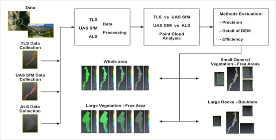
• Terrestrial laser scanner (TLS),
• Digital photogrammetry using UAS,
• Airborne laser scanning (ALS; Source of ALS products: ÚGKK SR; provided for our research by the Geodetic and Cartographic Institute of the Slovak Republic; described in [39]).

These three datasets were acquired in the same period; so it is possible to compare the created point-clouds in terms of vertical accuracy, point density, and DEM properties.

Aim of the Research

The goal of our research is to analyze the quality of the new national DEM 5.0 in terms of accuracy and detail by comparing with two other terrain representations—point clouds acquired by TLS and SfM aerial photogrammetry. They were created with a higher detail to monitor changes in the alpine landscape at a selected research site in the Small Cold Valley in the High Tatras, where research is underway to monitor the development of selected geohazards in the alpine environment. The identification of morphological changes in an alpine environment concerns in particular:

• Development of various geological phenomena such as weathering and movement of weathered material on a slope, development of erosion, etc.,
• The formation and development of geohazards such as landslides and falls, torrential rains and flash floods, and changes in the alpine landscape caused by them,
• Anthropogenic changes caused by human activity in urbanization and land use (construction of roads, sidewalks, construction of cottages, sports grounds, etc.).

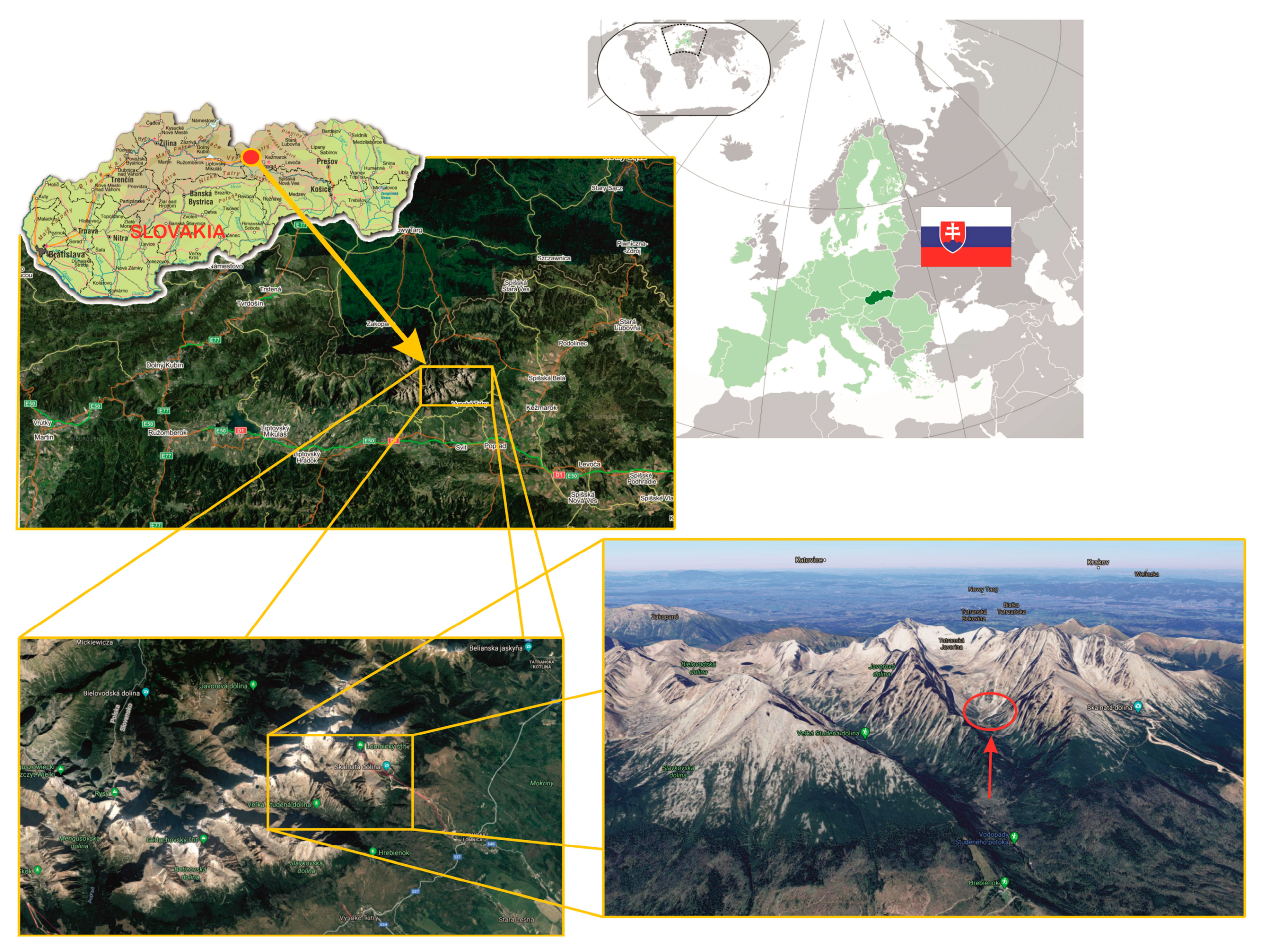
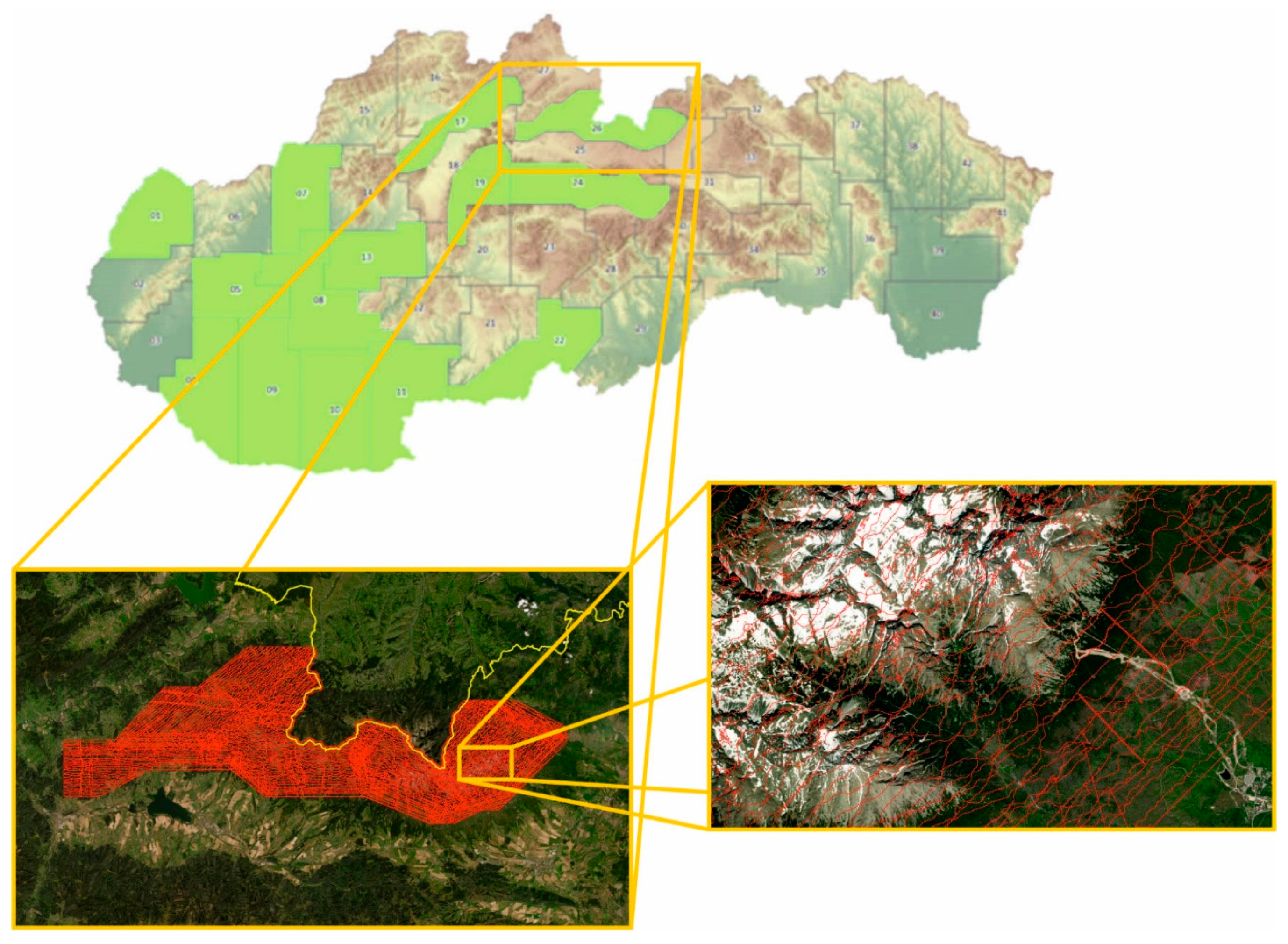
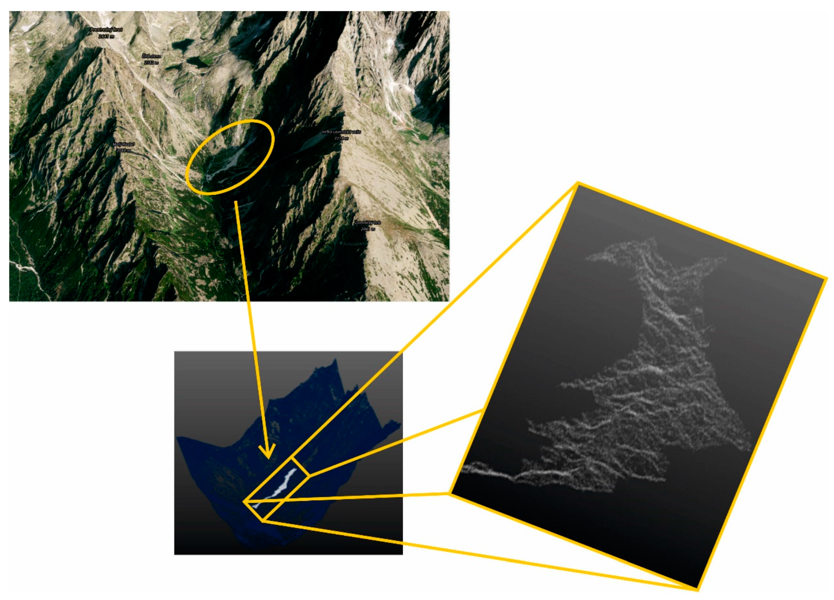
Our research also determines the size of measurable changes in surface morphology, or during the movement of variously large rock blocks in the alpine environment, that are identifiable from the national data provided by the Geodetic and Cartographic Institute of the Slovak Republic.

2. Study Area

2.1. Geographical Location

For our research, the Small Cold Valley (SCD) locality was selected (Figure 1). It is located in the north of Slovakia in the High Tatras mountains. The mountain massif measures approximately 26 km × 10 km. Since 1948, the area has been managed by the Tatra National Park—TANAP, with five levels of protection. The size of the national park is 73,800 ha. There are 25 peaks above 2500 m; the highest is Gerlachovský Peak with a height of 2654.4 m.

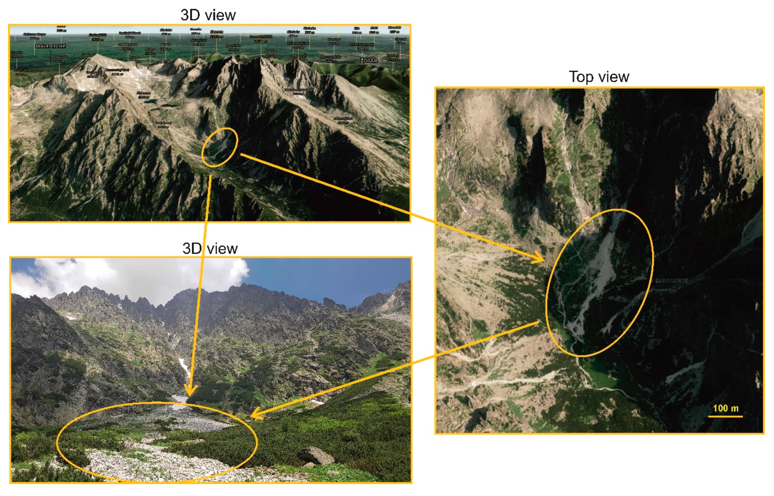
2.2. Description of the Study Area

In terms of the geomorphological division [40], the territory of the Tatras’ alpine landscape belongs to the Alpine-Himalayan system, the Carpathian subsystem, the province of the Western Carpathians. The Tatras’ alpine terrain is formed by the morphodynamic unit of the Tatras, approximately above the isohypse of 1500 m above sea level up to the highest position, while the highest point is the top of Gerlachovský Peak—2654.4 m above sea level. The alpine landscape of the Tatras is a precious area in terms of specific abiotic natural phenomena, typical of alpine areas, and the occurrence of rare and endemic flora. The whole area has been a part of the Tatra National Park since 1949 and since 1993 is included in the international list of Biosphere Reserves by UNESCO.

The alpine landscape can be stated as an area with a characteristic set of geological, morphodynamic, glaciological, climatic, pedological, botanical, zoological, and other features [41] and with a very high potential for tourism [42].

The valleys of the Tatra National Park can reach an altitude difference of 1000 m. Further transformation of the high-alpine surface’s topography is caused by weather, wind, and especially water erosion. This process continues currently, and it is possible to observe it mainly on the sidewalls of the valley and rock walls. Particularly significant are the talus cones, which are accumulation zones for the material washed out of the steep troughs. The occurrence of stone blocks and boulders is also frequent in the valleys.

The trigger for changes in the morphology of the landscape, especially in recent years, manifested on, for example, glacial moraines, rubble cones, and on boulders, are often recurring torrential rains supported by the simultaneous heating of the snow cover in the spring. In recent years, several massive rainfall events have been recorded in the High Tatras. During the last years, seasonal changes in the mountain riverbed are often visible to the naked eye, as well as changes in the shape of the talus cones in several TANAP valleys. The valleys are freely accessible to visitors of the national park along marked paths. The number of visitors is growing every year. There are often cases when hiking trails pass near mountain streams or unstable talus cones (Figure 2).

For our research, we chose locality with geographical position 49.186N, 20.208E at the end of the Small Cold Valley. It is located under the western wall of Lomnický Peak. The source area is located at an altitude of approximately 2200 m above sea level. The accumulation area is at the height of approximately 1600 m above sea level. Figure 3 shows an overall view of the SCD and the accumulation zone of the debris flow. Accumulation zone’s width is 20 m in the upper part and 80 m in the lower part. Size of stones is from a few centimeters to about 5 m (Figure 4). The site’s total length is about 400 m, and the area of the site is about 5000 m². The survey site is only accessible by a hiking trail. All instruments and surveying equipment had to be manually brought to the site. Even the all-day movement along the talus cone was physically and time-consuming.

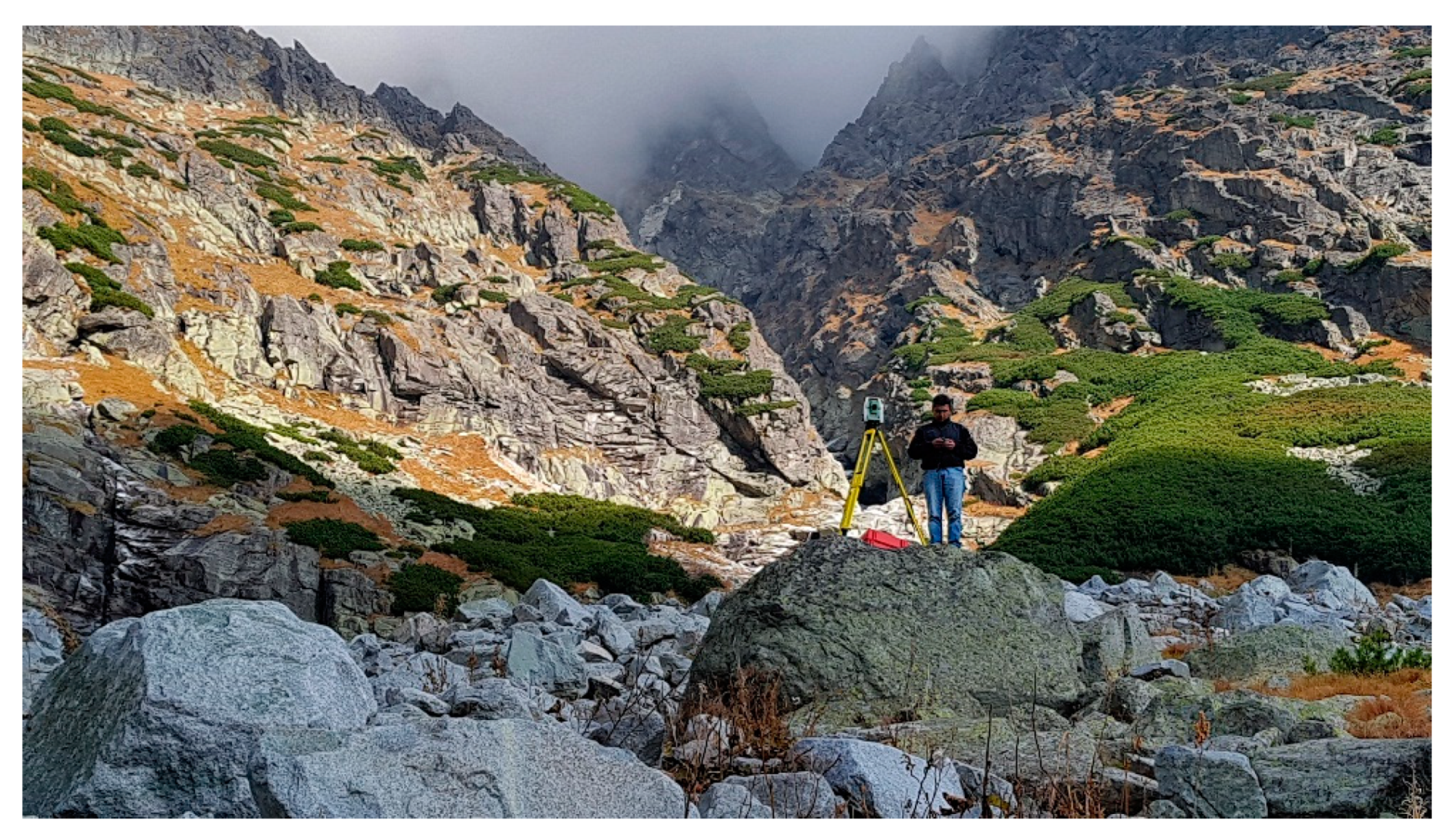
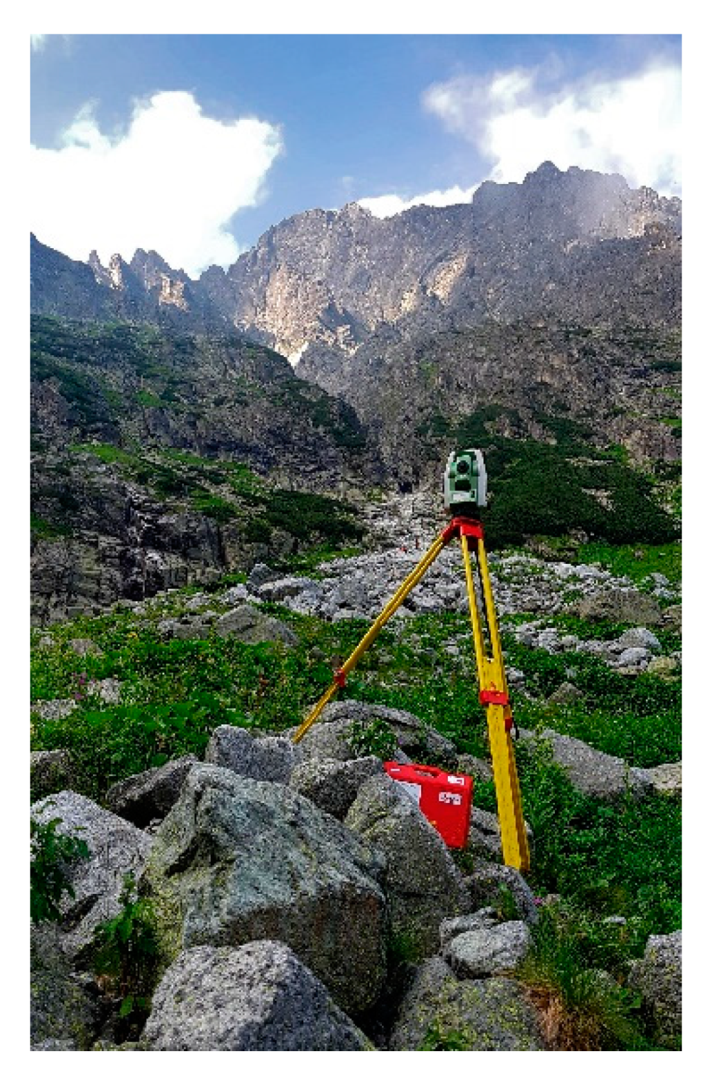
3. Field Surveying and Equipment

Geodetic and photogrammetric surveying methods were used to document the site’s current state and the generation of DEM. The survey aimed to capture the morphology of the terrain in detail. Used surveying methods allow direct measurement or generation of a point cloud. Point clouds obtained by different methods were mutually compared and analyzed in terms of detail and precision. Fieldwork was carried out in June 2018 according to the general procedure as follows:

• The survey project, determination of the extent of the area of interest, design, and deployment of the geodetic network based on available map materials.
• Monumentation and surveying of fixed points of the geodetic network.
• Determination of GCP coordinates for TLS and photogrammetry.
• TLS measurement and photogrammetric imaging.
• Control and verification measurement.

3.1. GNSS Surveying

GNSS measurements were realized to determine the coordinates of the initial survey points. These survey points were marked temporary. They were used to connect terrestrial measurements to the standard reference system in the Slovak Republic—Datum of Uniform Trigonometric Cadastral Network (S-JTSK) and Baltic Vertical Datum—after adjustment (Bpv). GNSS measurement was made by a Leica GPS900cs receiver using the RTK (real-time kinematic) method with connection to the Slovak Real-time Positioning Service (SKPOS). The standard deviation of these points was assumed to be 20 mm in position and 40 mm in height. Configuration of the fundamental geodetic network is shown in Figure 5.

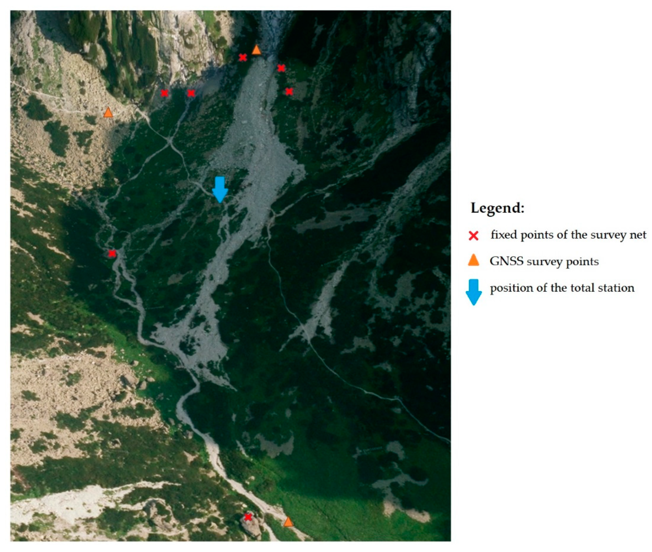
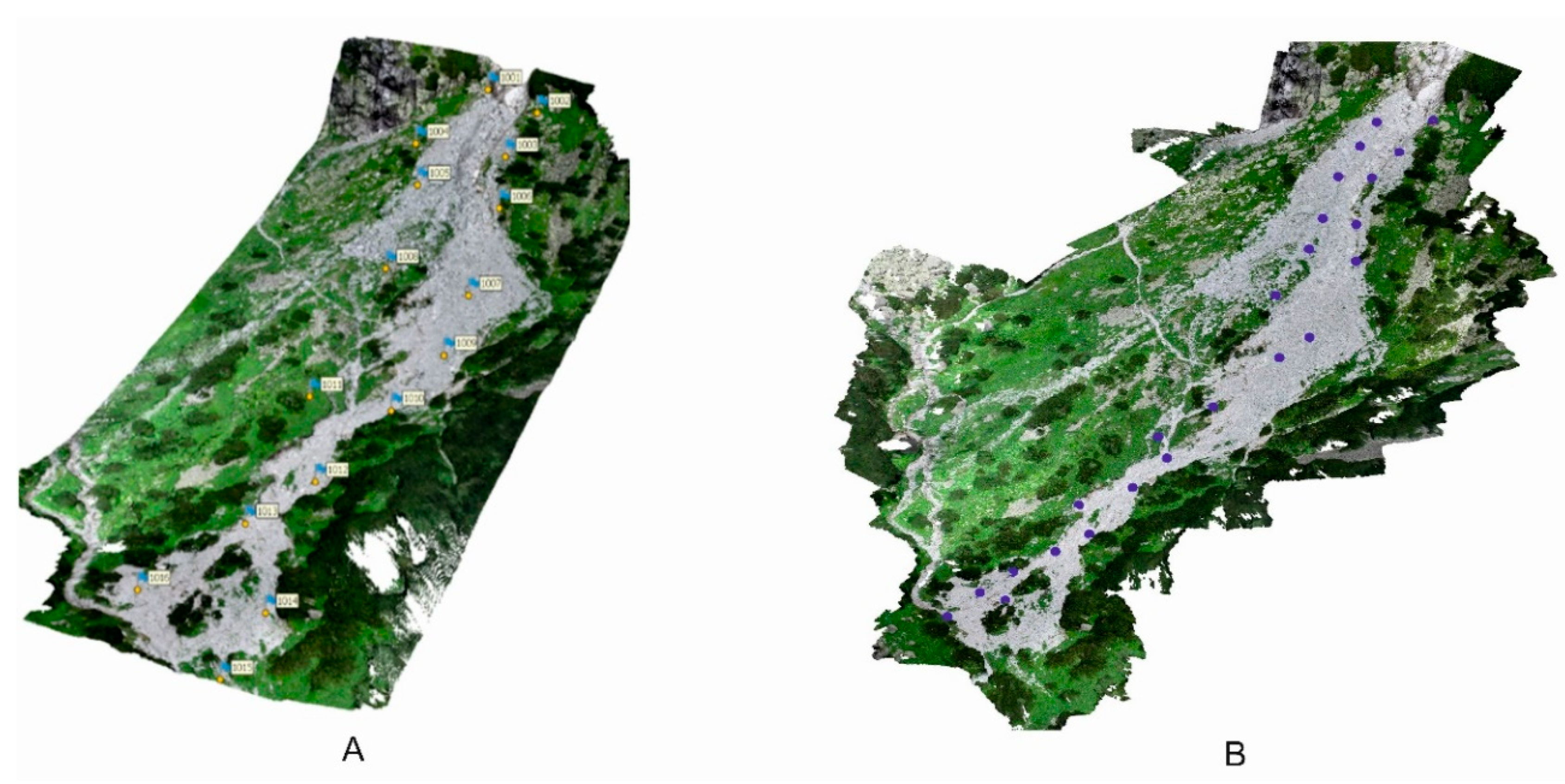
3.2. Geodetic Network and GCPs

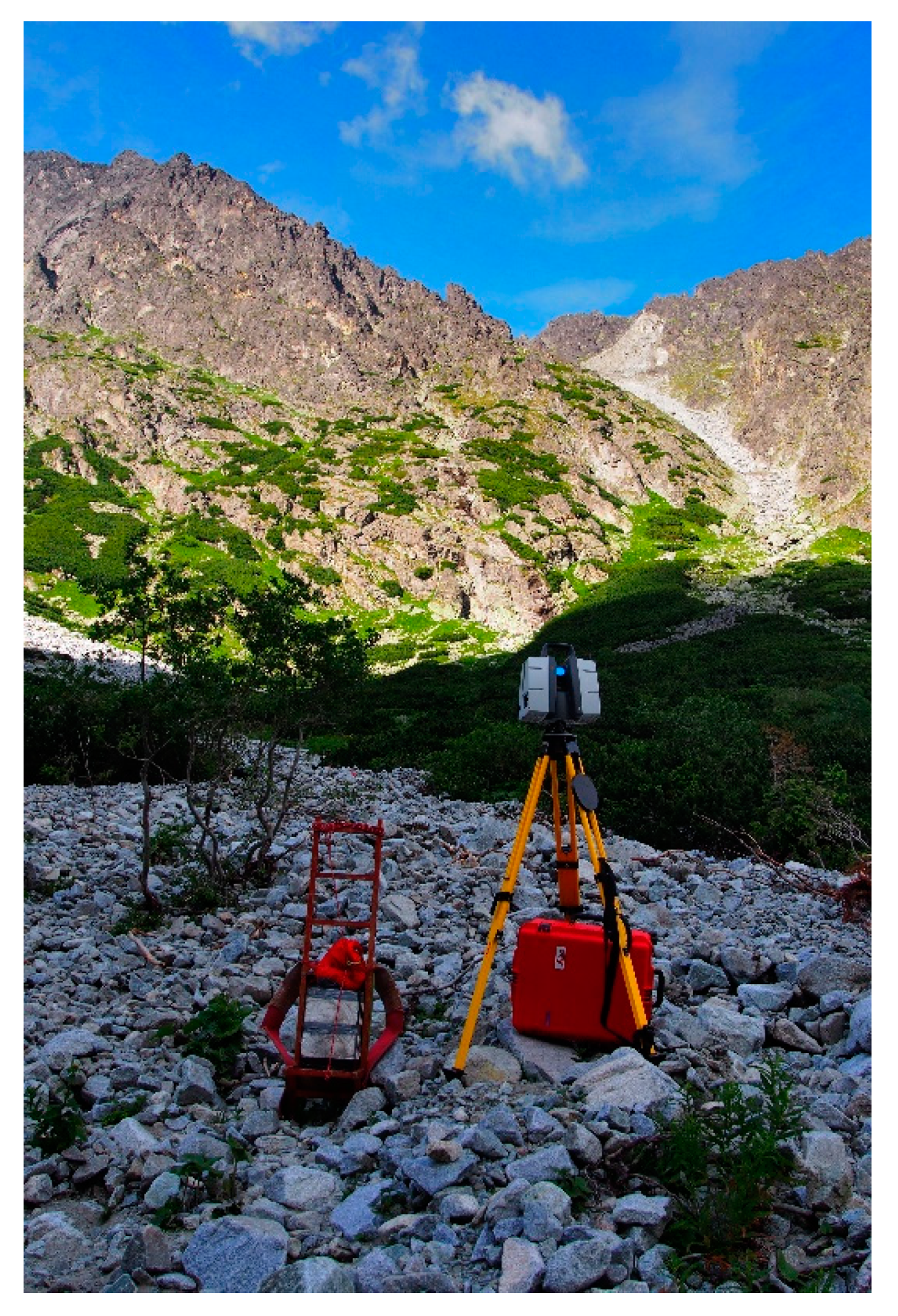
The total station Leica TS02 was used for the geodetic survey (Figure 6), with the horizontal direction and zenith angle measurement accuracy of 7″ (0.0020 gons) and the distance measurement accuracy of 1.5 mm + 2 ppm. Further parameters of the instrument are given in

Table 1. Leica TS02 characteristics.

Angle measurement (Hz, V)
Accuracy	7″
Distance measurement with a prism
Range	3500 m
Accuracy	1.5 mm + 2.0 ppm
Distance measurement without a prism
Range	>400 m
Accuracy	2 mm + 2 ppm

. The spatial coordinates of the survey station were determined from the GNSS initial survey points by the resection method. Position of the total station is indicated by a blue arrow in Figure 5. Fixed points of the survey net were stabilized by nails and retro-reflective targets on a compact rock outside of the active area of the talus cone. A red cross marks their position in Figure 5. The coordinates of these points were determined in three sets to increase the internal accuracy of the network points. The spatial position standard deviation of these points was up to 3 mm. These points form a precise fundamental geodetic network for further determination of ground control points.

The coordinates of GCPs were determined by the spatial polar method using TS02 with two faces survey mode. For the TLS survey, GCPs were determined during the TLS measurement procedure. Three Leica GZT21 HDS 4.5″ Black and White Scanning Targets were used. The reflector-less electronic distance measurement with the accuracy of 2 mm + 2 ppm was used. For photogrammetric measurements, GCPs were determined at once before photogrammetric imaging (Figure 7A). The GCPs were squared black and white, with dimensions 0.3 m × 0.3 m. The standard deviation of GCPs coordinate determination was up to 5 mm.

3.3. TLS Surveying

The Leica P40 terrestrial laser scanner (TLS) was used for a detailed measurement of the surface (Figure 8). Selected technical parameters are given in

Table 2. Leica P40 3D scanner characteristics.

Main Characteristics
Type	Time-of-flight laser scanner
Range and reflectivity	Minimum 0.4 m, 270 m@34%; 120 m@8%
Scan rate	Up to 1,000,000 points per sec
Field of view	H—360° (max.); V—290° (max.)
Accuracy
Distance measurement	1.2 mm + 10 ppm
Angular measurement	8″ horizontal; 8″ vertical
3D position	3 mm at 50 m; 6 mm at 100 m
Target acquisition	2 mm standard deviation at 50 m

.

For each scanner survey station (Figure 7B), at least three temporary Leica GZT21 HDS 4.5″ Black and White Scanning Targets were scanned separately. Coordinates of GCPs were determined by the TS during the TLS surveying. These points were used to register single point clouds to the common coordinate framework. Scanning resolution value was set to 12 mm at 10 m with a range of 120 m. Total of 25 survey stations (see Figure 7) were used, with a scanning time of about 12 h, which amounted (including transport and movement in the difficult terrain) to two working days.

We considered the TLS survey as a reference and validated method of measuring irregular objects. It is characterized by a high density and accuracy of the raster of measured points. Its disadvantage in the alpine environment is in addition to the demanding transport of the instrument and equipment. The terrain is rugged, measured from a small height above it, and therefore there are uncovered points in the surveyed area. To eliminate this, the number of standpoints would have to increase very much to survey the whole field. The TLS was, therefore, chosen as a control method for photogrammetric measurements using UAS.

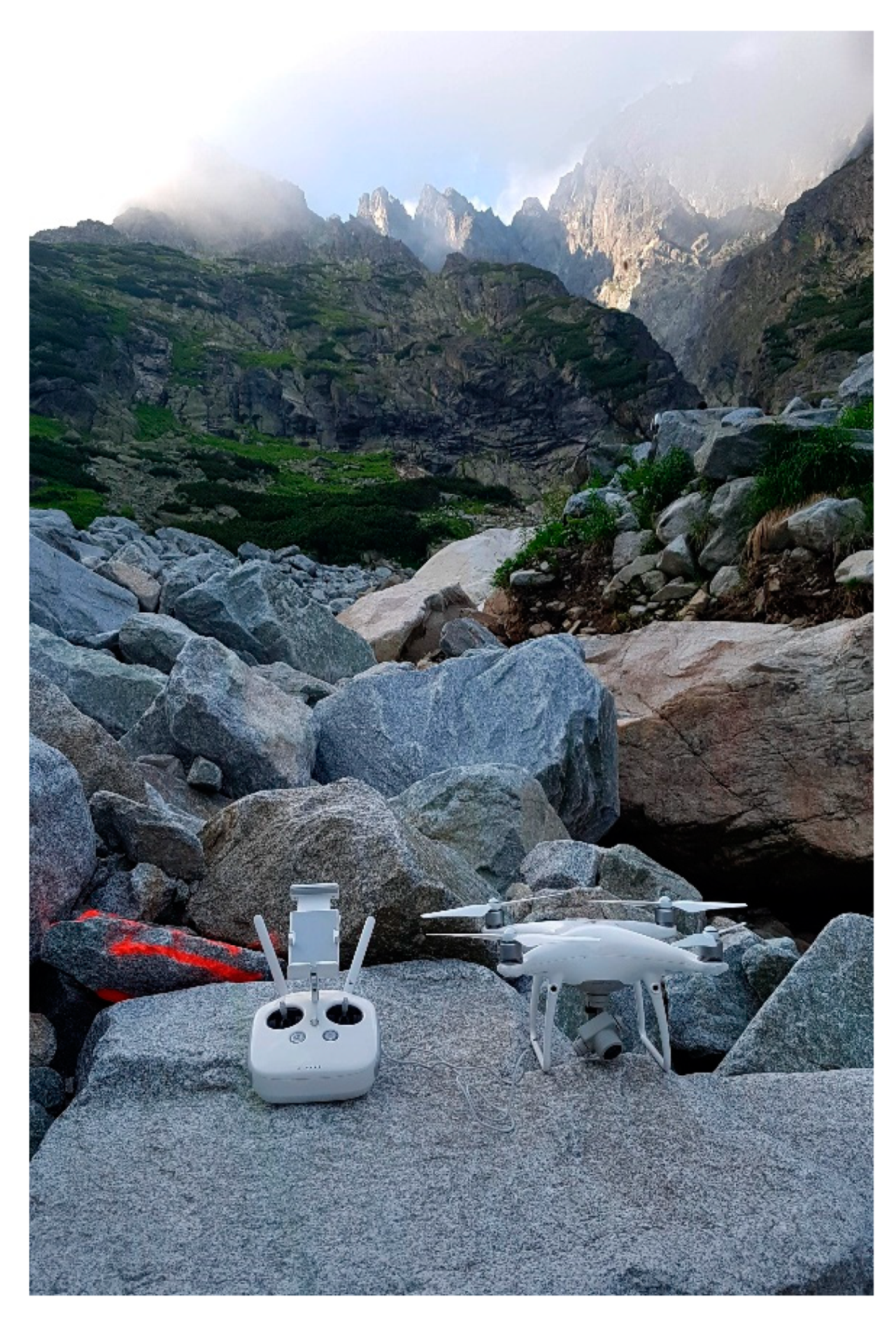
3.4. UAS Photogrammetry

The UAS DJI Phantom 4 Pro (Figure 9) equipped with a 5472 pixels × 3648 pixels digital camera was used to capture images covering talus cone under study. Further technical parameters are given in

Table 3. UAS DJI Phantom 4 Pro characteristics.

Aircraft
Weight (with Battery and Propellers):	1380 g
Max Ascent/Descent Speed:	6 m/s/4 m/s
Max Flight Speed:	20 m/s
Max. flight time:	28 min.
Satellite positioning system	GPS/GLONASS
Wind speed resistance	10 m/s
Camera
Operating Environment Temperature:	0–40 °C
Sensor:	1″ CMOS
Effective Pixels:	20 Megapixels
Image size:	4864 pixels × 3648 pixels (4:3)
Gimbal pitch	−90 to + 30°
Battery
Type	Li-Pol
Capacity	5870 mAh
Voltage	15.2 V

. Altogether, 1389 images were captured in several flights from an average height of 35 m above the ground (AGL), with the ground sampling distance (GSD) of approximately 0.01 m. The automatic camera mode with fixed ISO (100) was used during the flight (ISO 100, Shutter 1/60 to 1/800, F/3.5–F/7.1).

The goal was to obtain a point cloud of the entire talus cone with GSD up to 1 cm. Regarding the parameters of the camera, the flight altitude up to 35 m AGL was determined a priori. This height corresponds to a GSD of 0.95 cm/pix. Due to the extensive area of the territory—approximately 5000 m², and a height difference of 100 m between the upper and lower part, four separate flights were performed. The three flights were preprogrammed using the Pix4D field application so that the average flight altitude of 35 m was maintained in each of them. A double-grid pattern of the flight was used. Overlap of the images was set to 80%, gimbal pitch value 75°. The flights were performed in an automatic mode with a partial overlap. Last flight was performed using manual piloting of the UAS. During this flight, an effort was to maintain a height of up to 30 m AGL and cover the entire area in three strips with the camera’s orientation against the slope. Pitch value of the gimbal was set to 80°. The optical axis of the camera was, therefore, approximately perpendicular to the terrain. In total, 16 GCPs were used for georeferencing (Figure 7A). GCPs were distributed evenly throughout the area of interest. Total flight time was about 3 h.

4. Processing of Measured Data and Datasets

The TLS point cloud is intended to confirm compliance with the SfM point cloud obtained by UAS photogrammetry. The photogrammetric data will further form a reference point cloud for the analysis of the suitability and accuracy of the ALS data.

4.1. TLS Data Processing

Acquired scans were mutually registered and georeferenced in post-processing with use of HDS 4.5″ Black and White Scanning Targets. The scan registration residuals were below 3 mm for all 25 stations. The mean RMSE (root-mean-square error) was approximately 1.2 mm. Leica Cyclone 9.2 software was used for post-processing scan registration. The point cloud obtained from the TLS survey contained 597 million points. The mutual distance between individual points at most 5 mm. After removing vegetation, ground classification, the final point cloud contained 505 million points for further analysis (Figure 10left). Trimble Realworks^®® 10.0.4 software was used for point cloud editing. Despite the effort to continuously capture the area of interest, the TLS contains unmeasured areas (Figure 10right). The reason is the rugged terrain and the low position of the scanner on the tripod.

4.2. SfM Processing of Photogrammetric Data

The captured images were checked and sorted before further processing, with 1389 images entering the image processing. Agisoft Metashape Professional^®® ver. 1.5.0. software in the network configuration was used for the entire photogrammetric processing. Accuracy of the alignment of the images was set to the value high with generic pair preselection. Quality of dense cloud processing was set to a value high with mild depth filtering. The alignment of images was performed in one block at a time. Due to computational demand, the point cloud generation was divided into sub-blocks (so-called chunks) and subsequently combined into the one unit. The resulting point cloud contained 261 million points. After the ground classification and point cloud trimming according to the common area, the resulting point cloud contained 40 million points for further analysis (Figure 11left). In contrast to the TLS measurement, the area’s surface was covered continuously with a high level of detail. The mutual distance—the density of points was up to 10 mm (Figure 11right).

The quality of the photogrammetric model was verified during image processing using the Agisoft Metashape Professional^®® software ver. 1.5.0. The coordinates residuals on the ground control points were always less than 0.025 m, and the mean overall RMSE was 0.011 m; the RMSE of image coordinates was less than 0.32 pix, and the mean RMSE of coordinates was 0.16 pix. The verification of georeferencing was realized using checkpoints. The RMSE value at individual points was up to 0.030 m. Trimble Realworks^®® 10.0.4 software was used for the point-cloud segmentation.

4.3. Airborne Laser Scanning (ALS)

Since 2017, The Geodesy, Cartography, and Cadastre Authority of the Slovak Republic (ÚGKK SR) has been providing a new digital terrain model DMR 5.0 of the entire territory of the Slovak Republic, created from ALS data. The project should be completed in 2023. The whole area of the Slovak Republic is divided into 42 areas (Figure 12). Spatial data are provided to customers free of charge. The scanning takes place gradually in individual locations from the west of Slovakia to the east. The High Tatras location is placed in the area No. 26 with the time period of the ALS survey from June to September 2018 in three campaigns. Thus, DEMs that were compared were from the same period.

The ALS flight strips are shown in Figure 12. Area of interest is located in the centre of the image. It extends into 5 flight strips.

In addition to other topographic products, a classified point cloud in LAS 1.4 format is provided. ALS data provider supplies finished products (point clouds, DMR, and DMS). Available metadata are listed below. All of them are provided in the coordinate system Datum of Uniform Trigonometric Cadastral Network S-JTSK (implementation JTSK03) and Baltic Vertical Datum—After Adjustment (Bpv) and ETRS89-h. The Riegl LMS-Q780 sensor was used for the ALS. The average flight altitude was 3224 m AMSL (above mean sea level), with the average terrain altitude 1770 m AMSL, and the average flight altitude 1240 m AGL. The scanned strip’s average width was 1440 m. Size of the beam spot depends on the AGL flight height. The average value was 0.33 m. The average point density in the point cloud is 40 p/m². The density of ground points after the classification is a minimum of 14 p/m². The overlap of the scanned strips was more than 40%. The point cloud’s required absolute height standard deviation must be at least 0.15 m. but the standard deviation in height determined from the control measurements was 0.04 m.

Since the point cloud from ALS (Figure 13) was georeferenced in S-JTSK implementation JTSK03, and all our field measurements were referenced in newer S-JTSK implementation JTSK (which is slightly different), a transformation of points was necessary before further processing. Therefore, we used the authorized transformation service of the ÚGKK SR with the EPSG::8364 code for transformation. The most suitable input/output format for using the transformation service is the TXT file format, in this case. To make the transformed set compact as possible, it was trimmed according to the common area of interest, i.e., according to the TLS and SfM point clouds. Trimble Realworks^®® 10.0.4 software was used to edit the point cloud. The resulting point cloud contained 122,000 points with mutual distances of approximately 0.15 m, with continuous coverage but lower detail (Figure 13right).

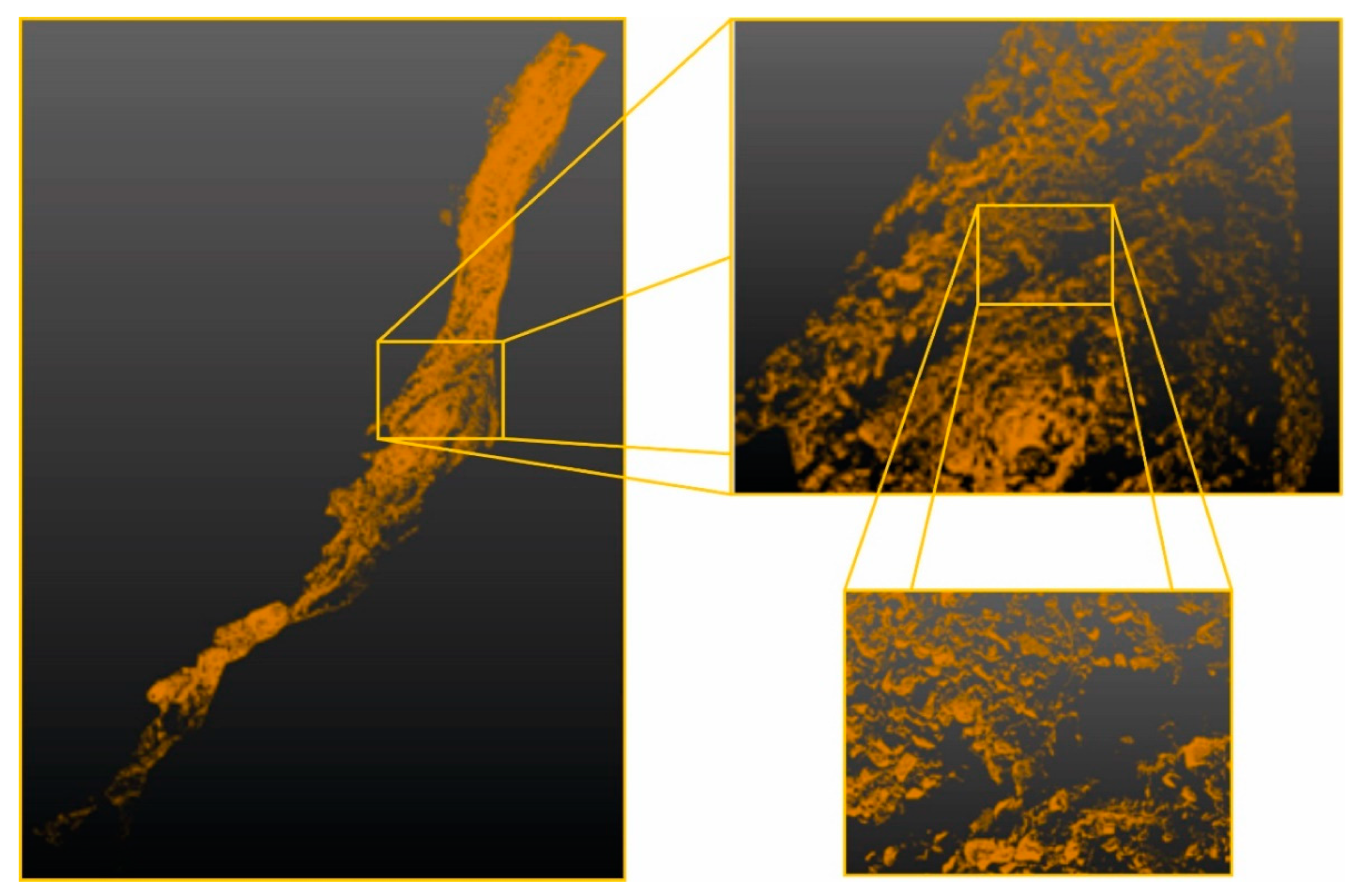
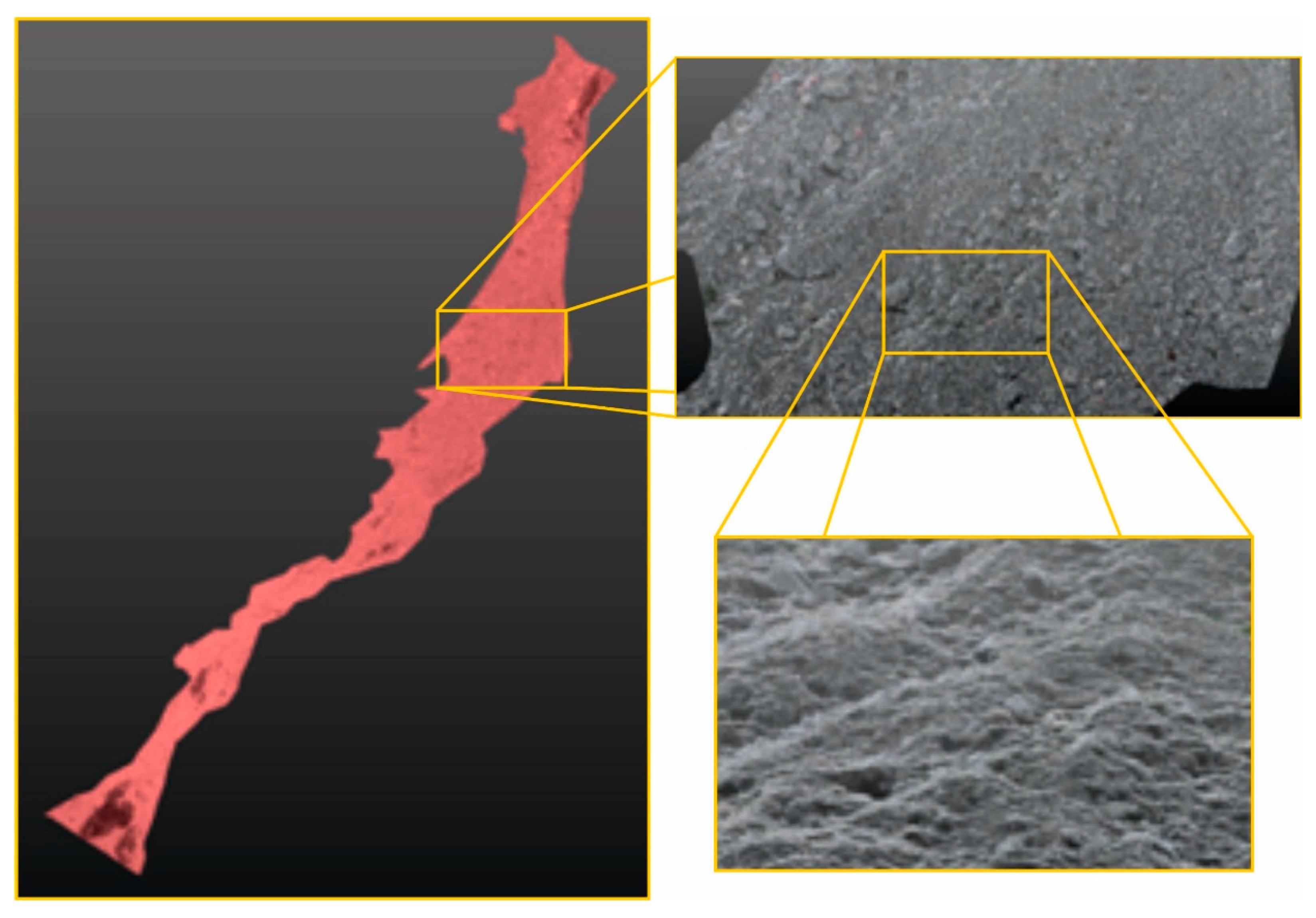
5. Analysis of Point Clouds and Results

We compared the sets of points obtained by TLS, UAS photogrammetry, and the ALS method with each other. The comparison of point clouds from TLS and UAS photogrammetry was intended to confirm the suitability and accuracy of the UAS approach. The reference and validated method, in this case, was TLS. In the case of expected compliance, the UAS SfM method’s point cloud would be considered the reference. Then, it could be compared with the results of the ALS in the area of interest.

After the dataset generation procedure, all datasets were trimmed to the study area border, and the analysis was performed using the trimmed datasets. From TLS and UAS datasets, the ground points were filtered for further evaluation. Trimble Realworks^®® 10.0.4. software was used. Properties and visuals of the datasets are shown in

Table 4. Properties of the datasets.

Dataset	Total Count of Points in the Raw Point Cloud	Count of Points in the Reduced Point Cloud	Average Point Cloud Density (point/m2)	Average Resolution of Point Cloud (m)	Spatial Sampling Resolution of Point Cloud (m)
TLS	505,000,000	5,486,311	1157	0.029	0.010
UAS	261,000,000	14,222,293	3000	0.018	0.010
ALS	190,000	82,764	17	0.243	0.150

and Figure 10, Figure 11 and Figure 13.

The average resolution of the point cloud (r) was determined from the point density (d) of the area of interest (points per m²) using the equation:

$$r=\frac{1}{\sqrt{d}},$$

(1)

Comparison of point clouds, creation of differential models and visualization of results were performed using 3DReshaper^®® 18.0.8 software. The numbers of points and their percentage in point clouds in mutual comparison were calculated using Trimble Realworks^®® 10.0.4 software. Standard deviations and point cloud distances were calculated by CloudCompare 2.10.2 software.

5.1. TLS vs. UAS Evaluation

5.1.1. The Whole Area

Figure 14left shows all TLS points compared to the points from UAS photogrammetry in terms of height. The range of the scale up to 600 mm corresponds to 100% TLS points and the maximum difference between clouds after ground filtration. Figure 14left shows that 98% of all values were in the range from −150 to +150 mm. The percentage of occurrence in the histogram indicates a systematic negative shift of point clouds. Over the entire area, two additional point cloud comparisons were made to verify the magnitude of the systematic shift. The extreme limits of comparison were set to values up to 150 mm (Figure 14middle) and up to 75 mm (Figure 14right). Figure 14middle shows that 97% of the points were in the range from −75 to +75 mm with a −7 mm systematic shift. Figure 14right shows that 91% of the points were in the range from −37.5 to +37.5 mm with a −6 mm systematic shift.

The standard height deviation of the whole area of the cone was 20 mm. This value was affected by incomplete removal of vegetation during ground filtration, incomplete TLS point cloud, height and geometry of the flight, generation of UAS point cloud, etc.

5.1.2. Partial Areas

Two parts of the talus cone were selected from the whole point cloud to confirm the standard deviation and systematic shift. Areas without vegetation were selected. Manual segmentation using Trimble Realworks software was used. The first one is a vegetation-free area of size 66 m². Figure 15 shows the comparison in terms of height; grey areas were not measured by TLS due to terrain topography. The histogram in Figure 15 with a scale range from −150 to +150 mm confirms the systematic shift of clouds with a value of −6 mm.

The second selected part for the point cloud comparison was a single boulder of size 6 m². The height component was compared (Figure 16). Areas not measured by the TLS were grey again. The histogram in Figure 16 with the range from −25 to +25 mm confirmed the systematic shift of clouds with a value of −6 mm. The standard deviation reached 20 mm.

Based on the results in

Table 5. TLS vs. UAS—results.

	Area (m2)	UAS Points	TLS Points	Mean (m)	Abs Max (m)	Std. Dev. (m)
Whole area	4400	14,222,293	5,486,311	−0.006	0.586	0.020
Vegetation-free	66	205,699	86,771	−0.006	0.149	0.022
Boulder	6	22,766	19,180	−0.006	0.030	0.018

, we considered the UAS point cloud verified. In further analyses, we considered it as reference for the analysis of the ALS cloud’s accuracy because due to the systematic shift of only −6 mm and the standard deviation of 20 mm, which are both values below the accuracy level of the GNSS RTK receiver.

5.2. UAS vs. ALS Evaluation

The comparison of UAS and ALS point clouds was realized similarly as in Section 5.1. representative smaller areas were selected for separate evaluation similar to the previous case.

5.2.1. The Whole Area

Figure 17 shows the height comparison of UAS and ALS point clouds of the entire site in the range of values up to 750 mm, up to 100 mm, up to 50 mm, and up to 10 mm.

Characteristics of point clouds and the results of surface analyses are given in

Table 6. SfM vs. ALS large areas—results.

	Area (m2)	UAS Points	ALS Points	Mean (m)	Abs Max (m)	Std. Dev. (m)
Whole area	4400	14,222,293	82,764	0.001	0.741	0.046
Vegetation free	1727	6,441,540	31,404	0.001	0.495	0.032

.

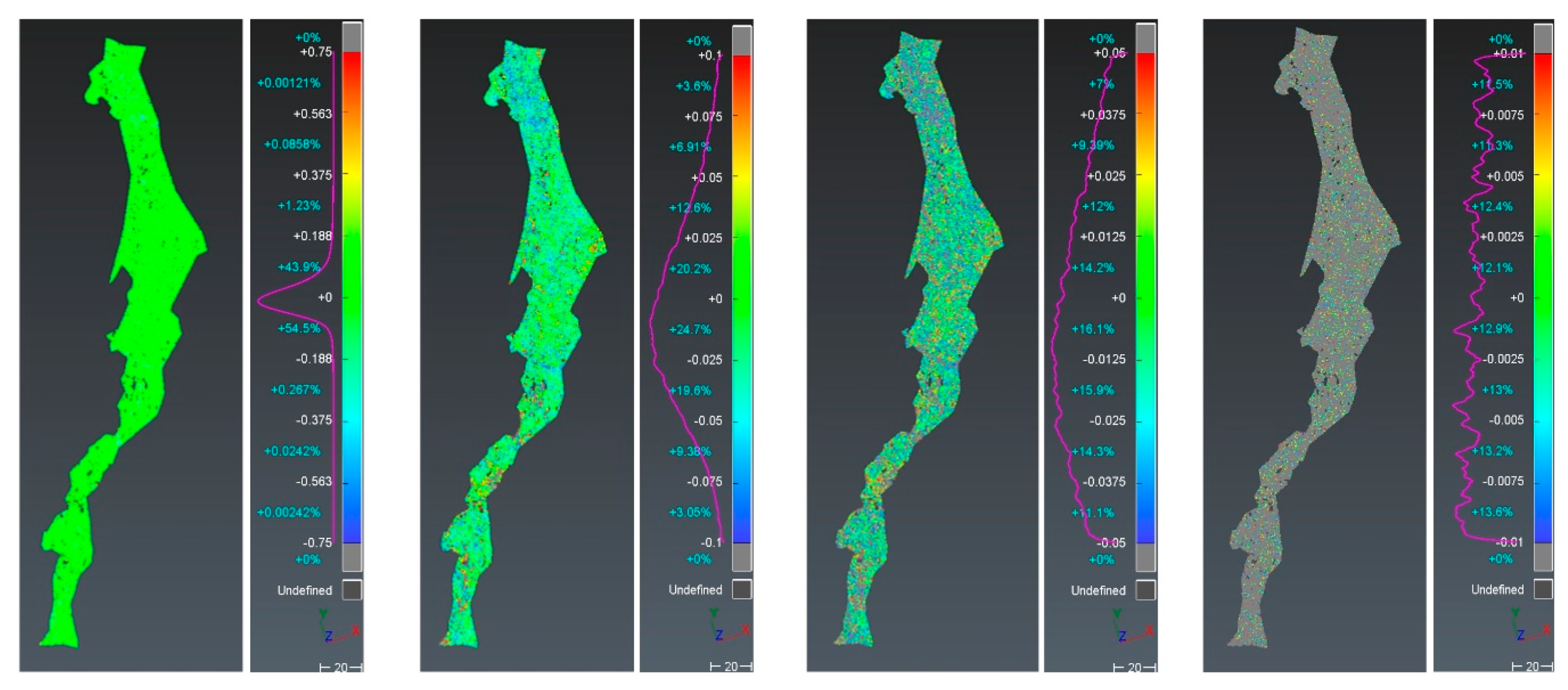
5.2.2. Large Vegetation-Free Area

For this analysis, a larger topographically complex vegetation-free area was segmented. Figure 18 shows the height comparison of UAS and ALS point clouds in the range up to 500 mm; 100 mm; 50 mm; and 10 mm. The UAS and ALS point cloud surface analysis shows that 96% of the points were within a distance of 100 mm, 77% of the points were within 50 mm, and 21% within 10 mm. Compared to the whole area comparison, we assumed a lower standard deviation. The results confirmed the assumption, and the results were better in all evaluated parameters. Characteristics of point clouds comparison are given in Table 6.

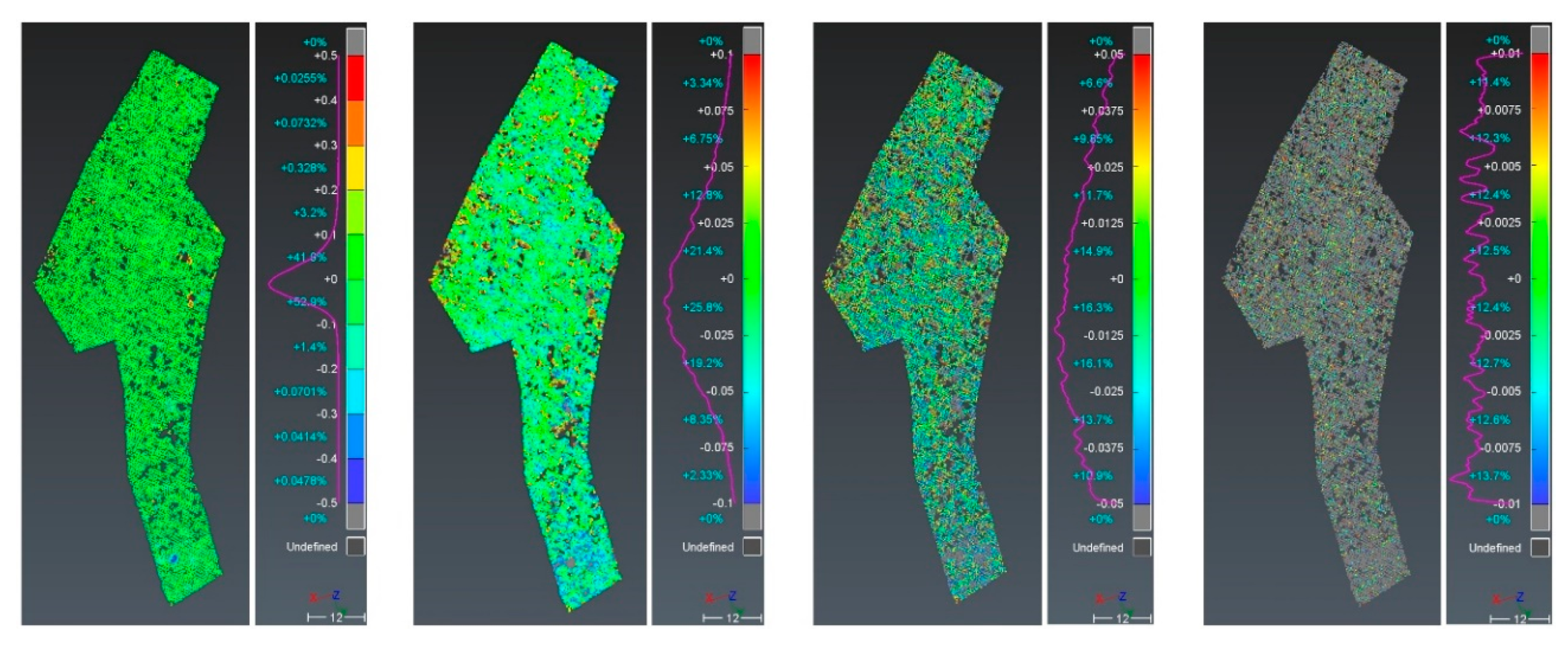
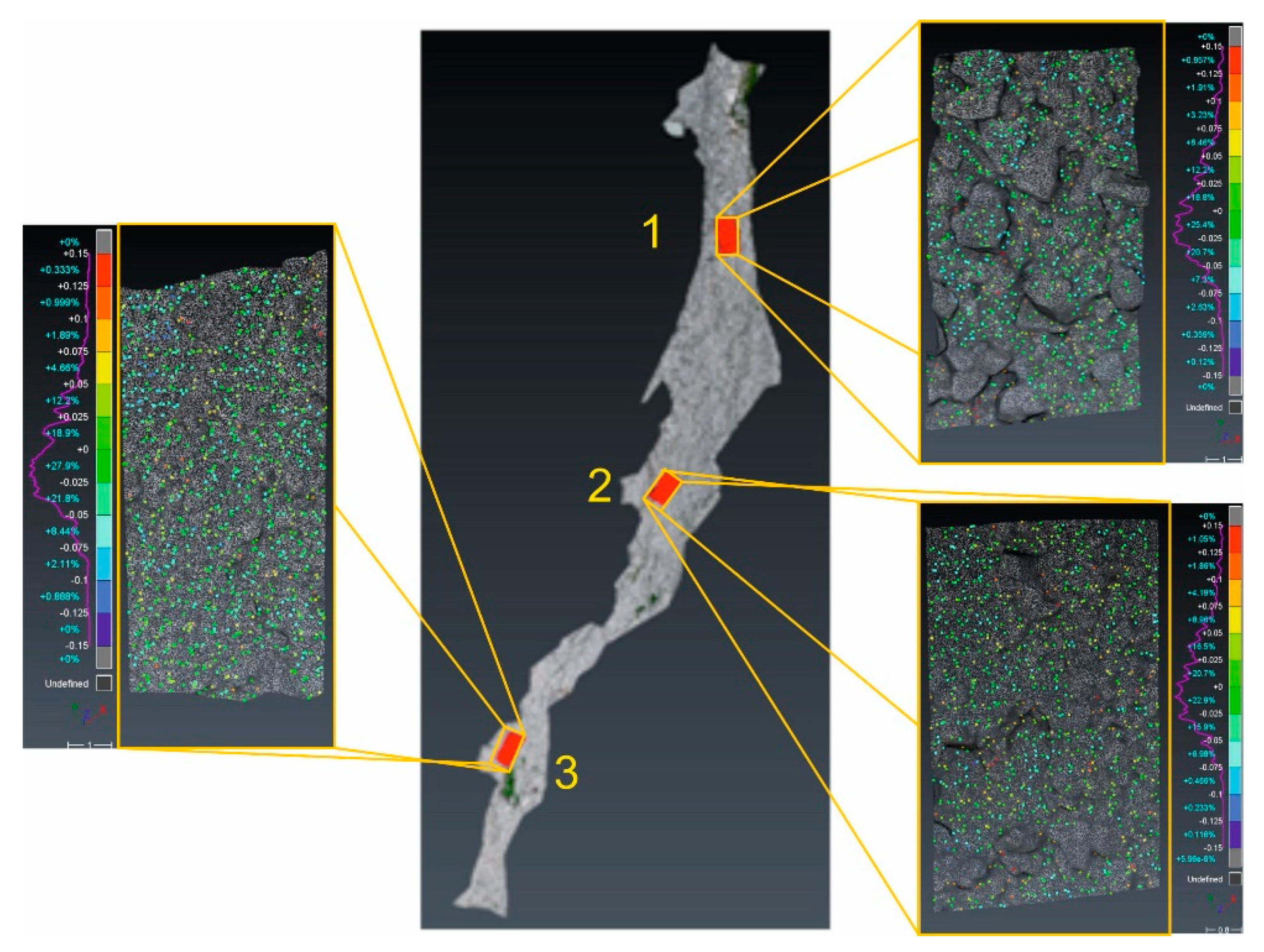
5.2.3. Small General Vegetation-Free Areas

Three different areas were selected for the analysis of smaller surfaces with a focus on high detail. Areas with different surface roughness were deliberately chosen, corresponding to the size of the rock debris fraction. Thus, there are various large cracks and gaps between the boulders. The size of the areas is approximately the same. According to Figure 3, the coarsest fraction is located at the top of the accumulation cone. In Figure 19, the surface No. 1 corresponded to this location. Surfaces Nos. 2 and 3 were successively finer fractions. The surface No. 2 was located in the middle part, and surface No. 3 was located in the lower part of the accumulation cone.

Figure 19 shows the height comparisons of UAS and ALS point clouds for all three areas up to 150 mm. The characteristics of the point clouds and the results of the analysis are stated in

Table 7. UAS vs. ALS for small general areas without vegetation—results.

Area	Area (m2)	UAS Points	ALS Points	Mean (m)	Abs Max (m)	Std. Dev. (m)
1	66	205,699	842	0.015	0.178	0.033
2	47	149,748	862	0.016	0.155	0.033
3	42	114,623	901	0.017	0.114	0.033

. The height difference standard deviation was 33 mm for all three partial areas. This value was better than the whole area and approximately the same compared to the large area without vegetation. The mean value ranged from 15 to 17 mm.

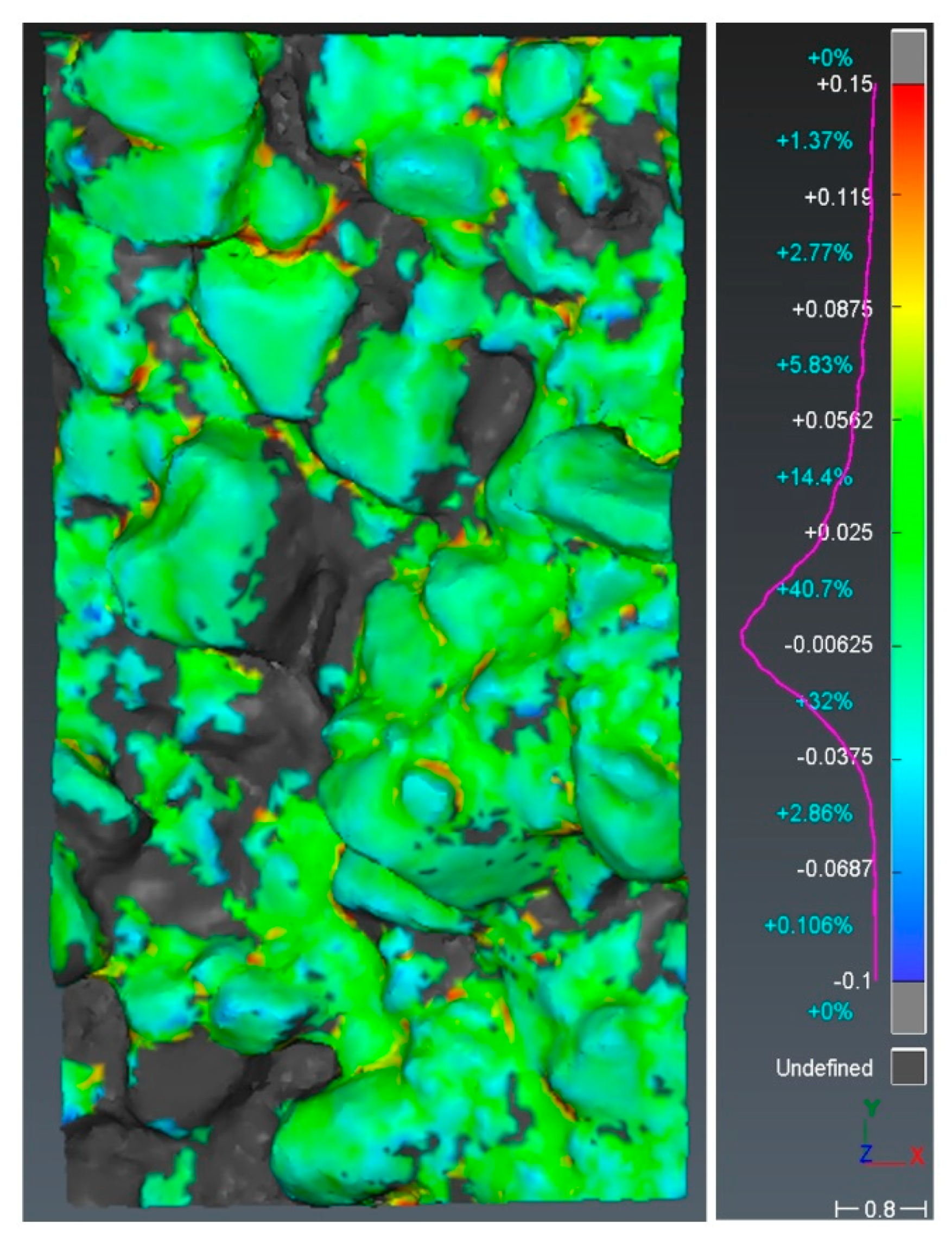
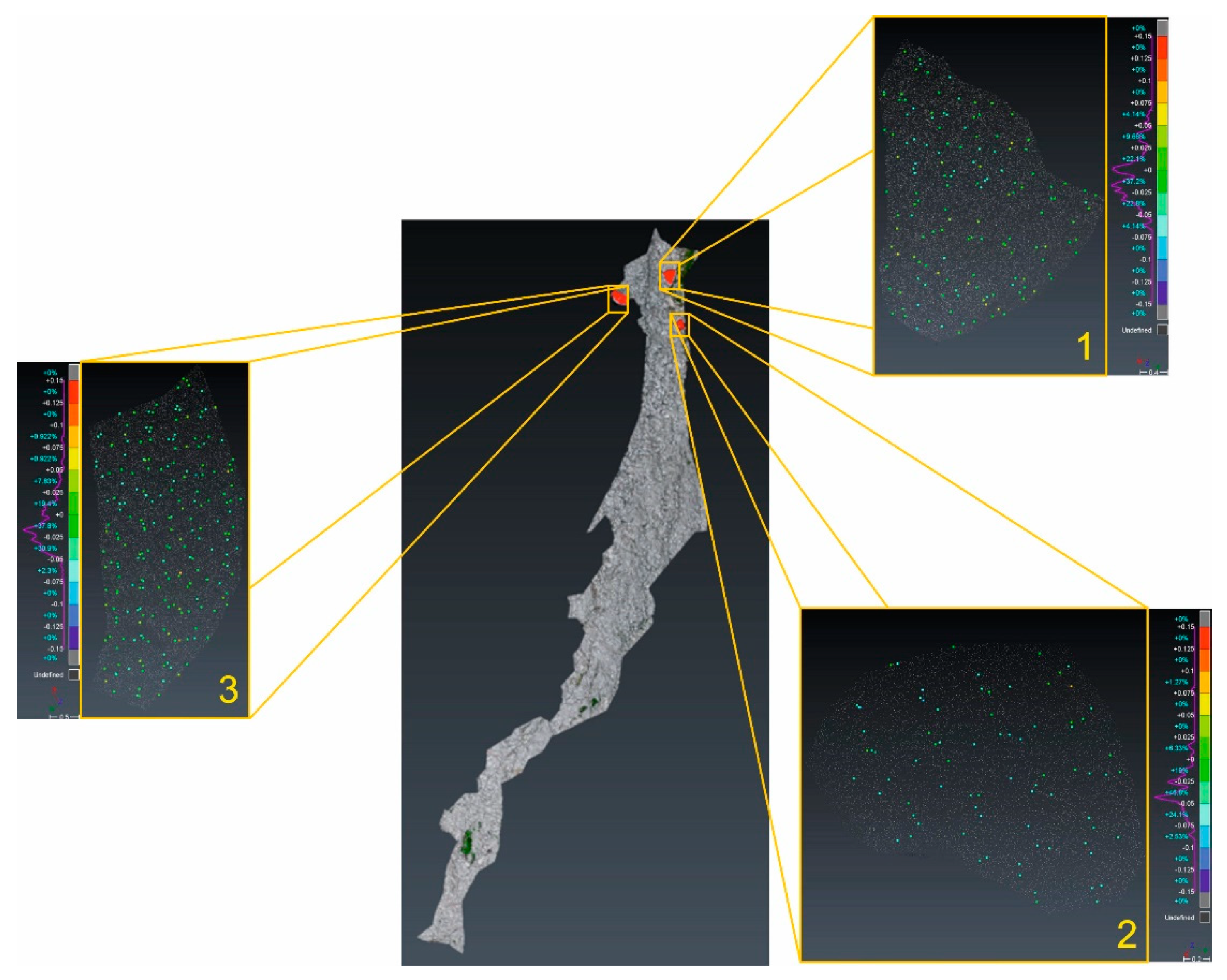
5.2.4. Large Rocks—Boulders

These were located only in the upper part of the cone accumulation zone. The three largest boulders were chosen (Figure 20). The surface of the boulders was evenly rounded and slightly rugged.

Figure 20 shows the UAS and ALS point clouds comparisons. Three boulders with differences in the range up to 150 mm were evaluated. Characteristics of point clouds and the results of the analysis are stated in

Table 8. UAS vs. LLS for boulders—results.

Boulder	Area (m2)	UAS Points	ALS Points	Mean (m)	Abs Max (m)	Std. Dev. (m)
1	12	22,766	154	0.015	0.100	0.022
2	6	7712	85	0.029	0.106	0.026
3	15	27,003	217	0.010	0.109	0.019

. Values of height differences were in the range of 19–26 mm. The mean value was from 10 to 29 mm.

6. Discussion

We considered the TLS measurement as a reference method from the point of view of measurement accuracy. High accuracy results from the accuracy parameters of the instrument and the possibility of connecting the survey to an accurate surveying net in the field. The advantage is also the fact that the result is just a georeferenced point cloud.

The disadvantage is a high purchase cost of the instrument, and the need to perform measurements from a higher number of scanning stations, which extends the time required for measurements in the field. In our case, we performed measurements from 20 scanning stations in one day. Even with great effort, it is not possible to target a location completely without missing data in the final point cloud. With regard to the complexity of the terrain, the high weight of the instrument can also be considered as a disadvantage.

The main advantages of aerial SfM photogrammetry are the speed of measurement in the field; the completeness of the final data; high density of the obtained point cloud; and the low cost of the used UAS. The main disadvantages are higher hardware requirements for image processing and longer office work time.

The ALS measurement was performed without a direct presence in the field. Since the data is provided free of charge, it is considered as the “cheapest” method. However, a problem of the source we used is an update of the data. The disadvantage is also the lower density of the point cloud.

The accuracy in the points of the terrain acquired by the ALS method was practically comparable to the most accurate commonly available method of terrestrial laser scanning (Leica P40), and UAS photogrammetry—the standard deviation of the height differences over the entire compared area was 20 mm. The systematic shift value was determined −6 mm.

It was necessary to consider that coordinates of the points derived by any method compared in this research as influenced by the accuracy of georeferencing into a common coordinate system (S-JTSK and Bpv). This analysis was practically performed based on GNSS-RTK measurements. It can be visible mainly in the average value of the shift.

In [43,44,45], we focused on the evaluation of surfaces obtained by the UAS-SfM method against surfaces obtained by the spatial polar method using the total station at specific points. The achieved standard deviations of height differences were comparable to the values presented in these research works.

The authors in [43] compared the surfaces obtained by the TLS survey against the surfaces from the SfM method obtained by different instruments at different flight altitudes. By comparing the differences of our TLS and SfM surfaces in the Z (height) component, we achieved smaller differences and a lower standard deviation at a comparable UAS flight altitude when compared to [43]. We also compared the surfaces obtained by TLS and SfM in [38]. Suitability of use of UAS for determining deformations of the land surface was verified in the context of mining activities in [46].

Based on point cloud analysis we determine, that the average systematic displacement for the whole area was 1 mm and the standard deviation was 46 mm. Two point clouds were compared, first obtained by ALS with an average flight altitude of 1240 m above terrain and second point cloud obtained by SfM from UAS with an average flight altitude about 30 m. When comparing the area without vegetation, the value of the systematic shift was the same; the standard deviation was even better—32 mm. These findings suggest that if such globally acquired data are available, in many cases, no further measurement is required (such as detailed mapping to determine contour lines). The main difference here was the density of coverage, where the ALS method provided (see used data) an average of 17 points per m² (with spacing 0.24 m). ALS was therefore suitable for documenting objects larger than 1 m². On the other hand, the UAS SfM method could provide 3000 points per m² (with spacing 0.02 m) and it is ideal for monitoring even small morphological changes on the surface or objects.

The suitability of ALS technology is also highlighted by authors in [47] to detect morphogenetic processes and map debris flows based on DTM derived from the ALS survey. Furthermore, authors in [36] demonstrated the usability and quality of TLS and UAS photogrammetry’s combination to derive a high-resolution DEM for a complex alpine environment.

When comparing the ALS method’s achieved results, for example, with [48], where the achievable accuracy of ALS measurements on a bridge structure (flat surface) was evaluated, the following resulted. The scanning was performed with a Riegl LMS-Q680i instrument as part of the measurements performed by PZGiK (Polish State Geodetic and Cartographic resource) at the height of about 1000 m and with a track size (diameter) of 0.5 m. The accuracy in the order of centimeters was achieved.

Achievable accuracies were also tested in [9]. Accuracy of 0.032 m was achieved with a Riegl LMS-Q680i scanner when monitoring the debris slide on the side of the valley at an altitude of 700 to 1000 m AGL. Additionally, in [19], the RMSD accuracy of up to 0.04 m was achieved when monitoring burnt areas in the tropics.

From the above information, it follows that our experiment results correspond to the accuracy achieved in the experiments of other authors. Our results confirm the achievement of accuracy even on difficult terrain and are significantly better than stated by the provider.

In our further research of the site, we plan to involve the combined use of remote sensing methods—aerial and terrestrial digital photogrammetry with the SfM approach with TLS and ALS data especially for surveying the details of the talus cone, similar to the works [36,49,50] with appropriate modifications.

7. Conclusions

A comparison of measurement methods (TLS, UAS, and ALS) was performed for monitoring or mapping specific landslide areas. Part of the area in the Small Cold Valley in the High Tatras was used for testing, specifically, it is a talus cone formed by stones of various sizes (from boulders to coarse gravel). The authors of the article obtained TLS and UAS data, ALS data were obtained from publicly available sources—national DEM 5.0 of Slovak Republic provided by the local authority.

The comparison was made on point clouds. The achieved accuracy of the height component of individual methods was comparable; the systematic shift was in the range of units of centimeters, the standard deviation was then in the range of 0.03–0.05 m. These values were fundamentally affected by the accuracy of georeferencing using GNSS. The details of land capture already differed significantly, where the UAS method could easily achieve a uniform density of several thousand points per m² (3000 per m², i.e., resolution 0.02 m), the TLS method could achieve similar values. The coverage was very uneven due to frequent obstacles. ALS data had a much lower density; in our case, 17 points per m² (resolution 0.243 m), the coverage was also uniform. Use of the TLS method differed from the other two approaches in terms of difficultness of the measurement. The instrument was placed at a small height, and due to the obstacles in rugged terrain, a large number of standpoints and measurements would be needed to capture entire area without neglected gaps in the point cloud. For the UAS and ALS methods, the terrain fragmentation practically did not matter.

All methods were in principle applicable for capturing the state of a highly specific area of a rubble cone, with TLS being application problematic. Thus the most suitable technology is UAS, which is very flexible and fast to use, inexpensive, and provides high point cloud density. On the other hand, publicly available ALS data showed comparable accuracy (higher than stated by the provider), limited only by the lower density and update interval of the data.

These advantages and/or disadvantages determine the ALS technology for documenting changes in the country, namely: morphological changes on “continuous surfaces” such as talus cones, rock moraines, river terraces, and alluvial cones but of course also soil cover or rock massifs, and movement of rock blocks, or change of position of any natural or anthropogenic objects with a size from approximately 1 m².

Our research should serve as a basis for further stage measurements of land changes or the development of selected geohazards in a hardly accessible terrain (alpine environment, national parks, and non-urbanized landscape) with the following conclusions:

• Our results confirmed the suitability of the ALS method,
• Advantages of ALS are the speed of data collection over a large area at the same time,
• ALS data collection eliminates the need for demanding field data collection in inaccessible locations, hardly accessible and dangerous terrain such as mountain gutters, active talus cones, or in alpine environments, where it is difficult or even impossible to transport geodetic instruments,
• ALS makes it easy to perform repeated measurements or to plan stage surveys at preplanned intervals,
• The main disadvantages of ALS are the lower detail of the DEM and significantly higher financial demands.

References

1. Sepúlveda, S.A.; Alfaro, A.; Lara, M.; Carrasco, J.; Olea-Encina, P.; Rebolledo, S.; Garcés, M. An active large rock slide in the Andean paraglacial environment: The Yerba Loca landslide, central Chile. Landslides 2020. [Google Scholar] [CrossRef]
2. Chang, K.-J.; Tseng, C.-W.; Tseng, C.-M.; Liao, T.-C.; Yang, C.J. Application of Unmanned Aerial Vehicle (UAV)-Acquired Topography for Quantifying Typhoon-Driven Landslide Volume and Its Potential Topographic Impact on Rivers in Mountainous Catchments. Appl. Sci. 2020, 10, 6102. [Google Scholar] [CrossRef]
3. Hofierka, J.; Gallay, M.; Bandura, P.; Šašak, J. Identification of karst sinkholes in a forested karst landscape using airborne laser scanning data and water flow analysis. Geomorphology 2018, 308, 265–277. [Google Scholar] [CrossRef]
4. Available online: https://www.europeandataportal.eu (accessed on 23 November 2020).
5. Moudrý, V.; Urban, R.; Štroner, M.; Komárek, J.; Brouček, J.; Prošek, J. Comparison of a commercial and home-assembled fixed-wing UAV for terrain mapping of a post-mining site under leaf-off conditions. Int. J. Remote Sens. 2019, 40, 555–572. [Google Scholar] [CrossRef]
6. Štroner, M.; Urban, R.; Reindl, T.; Seidl, J.; Brouček, J. Evaluation of the Georeferencing Accuracy of a Photogrammetric Model Using a Quadrocopter with Onboard GNSS RTK. Sensors 2020, 20, 2318. [Google Scholar] [CrossRef] [Green Version]
7. Benjamin, A.R.; O’Brien, D.; Barnes, G.; Wilkinson, B.E.; Volkmann, W. Improving data acquisition eficiency: Systematic accuracy evaluation of GNSS-assisted aerial triangulation in UAS operations. J. Surv. Eng. 2020, 146, 1–15. [Google Scholar] [CrossRef]
8. Bruggisser, M.; Hollaus, M.; Kükenbrink, D.; Pfeifer, N. Comparison of Forest Structure Metrics Derived from UAS LiDAR and ALS Data. ISPRS Ann. Photogramm. Remote Sens. Spat. Inf. Sci. 2019, IV-2/W5, 325–332. [Google Scholar] [CrossRef] [Green Version]
9. Zieher, T.; Bremer, M.; Rutzinger, M.; Pfeiffer, J.; Fritzmann, P.; Wichmann, V. Assessment of landslide-induced displacement and deformation of above-ground objects using UAS-borne and airborne laser scanning data. ISPRS Ann. Photogramm. Remote Sens. Spat. Inf. Sci. 2019, IV-2/W5, 461–467. [Google Scholar] [CrossRef] [Green Version]
10. Thiel, C.; Schmullius, C. Derivation of Forest Parameters from Stereographic UAS Data—A Comparison with Airborne Lidar Data. Available online: https://ui.adsabs.harvard.edu/abs/2016ESASP.740E.189T/abstract (accessed on 5 November 2020).
11. Tournadre, V.; Pierrot-Deseilligny, M.; Faure, P.H. UAS Photogrammetry to Monitor Dykes—Calibration and Comparison to Terrestrial Lidar. Int. Arch. Photogramm. Remote Sens. Spat. Inf. Sci. 2014, XL-3/W1, 143–148. [Google Scholar] [CrossRef] [Green Version]
12. Grohmann, C.H.; Garcia, G.; Affonso, A.A.; Albuquerque, R.W. Dune migration and volume change from airborne LiDAR, terrestrial LiDAR and Structure from Motion-Multi View Stereo. Comput. Geosci. 2020, 143, 104569. [Google Scholar] [CrossRef]
13. Wallace, L.; Lucieer, A.; Malenovský, Z.; Turner, D.; Vopěnka, P. Assessment of Forest Structure Using Two UAS Techniques: A Comparison of Airborne Laser Scanning and Structure from Motion (SfM) Point Clouds. Forests 2016, 7, 62. [Google Scholar] [CrossRef] [Green Version]
14. Cao, L.; Liu, H.; Fu, X.; Zhang, Z.; Shen, X.; Ruan, H. Comparison of UAS LiDAR and Digital Aerial Photogrammetry Point Clouds for Estimating Forest Structural Attributes in Subtropical Planted Forests. Forests 2019, 10, 145. [Google Scholar] [CrossRef] [Green Version]
15. Moe, K.T.; Owari, T.; Furuya, N.; Hiroshima, T. Comparing Individual Tree Height Information Derived from Field Surveys, LiDAR and UAS-DAP for High-Value Timber Species in Northern Japan. Forests 2020, 11, 223. [Google Scholar] [CrossRef] [Green Version]
16. Pellicani, R.; Argentiero, I.; Manzari, P.; Spilotro, G.; Marzo, C.; Ermini, R.; Apollonio, C. UAS and Airborne LiDAR Data for Interpreting Kinematic Evolution of Landslide Movements: The Case Study of the Montescaglioso Landslide (Southern Italy). Geosciences 2019, 9, 248. [Google Scholar] [CrossRef] [Green Version]
17. Salach, A.; Bakuła, K.; Pilarska, M.; Ostrowski, W.; Górski, K.; Kurczyński, Z. Accuracy Assessment of Point Clouds from LiDAR and Dense Image Matching Acquired Using the UAS Platform for DTM Creation. ISPRS Int. J. Geo-Inf. 2018, 7, 342. [Google Scholar] [CrossRef] [Green Version]
18. Borrelli, L.; Conforti, M.; Mercuri, M. LiDAR and UAS System Data to Analyze Recent Morphological Changes of a Small Drainage Basin. ISPRS Int. J. Geo-Inf. 2019, 8, 536. [Google Scholar] [CrossRef] [Green Version]
19. Kociuba, W. Different Paths for Developing Terrestrial LiDAR Data for Comparative Analyses of Topographic Surface Changes. Appl. Sci. 2020, 10, 7409. [Google Scholar] [CrossRef]
20. Derrien, A.; Villeneuve, N.; Peltier, A.; Beauducel, F. Retrieving 65 years of volcano summit deformation from multitemporal structure from motion: The case of Piton de la Fournaise (La Réunion Island). Geophys. Res. Lett. 2015, 42, 6959–6966. [Google Scholar] [CrossRef] [Green Version]
21. Jovančević, S.D.; Peranić, J.; Ružić, I.; Arbanas, Ž. Analysis of a historical landslide in the Rječina River Valley, Croatia. Geoenviron. Disasters 2016. [Google Scholar] [CrossRef] [Green Version]
22. Rossi, G.; Tanteri, L.; Tofani, V.; Vannocci, P. Multitemporal UAS surveys for landslide mapping and characterization. Landslides 2018, 15, 1045. [Google Scholar] [CrossRef] [Green Version]
23. Ridolfi, E.; Buffi, G.; Venturi, S.; Manciola, P. accuracy analysis of a dam model from drone surveys. Sensors 2017, 17, 1777. [Google Scholar] [CrossRef] [PubMed] [Green Version]
24. Buffi, G.; Manciola, P.; Grassi, S.; Barberini, M.; Gambi, A. Survey of the Ridracoli Dam: UAS–based photogrammetry and traditional topographic techniques in the inspection of vertical structures. Geomat. Nat. Hazards Risk 2017, 1562–1579. [Google Scholar] [CrossRef] [Green Version]
25. Duró, G.; Crosato, A.; Kleinhans, M.G.; Uijttewaal, W.S.J. Bank erosion processes measured with UAS-SfM along complex banklines of a straight mid-sized river reach. Earth Surf. Dyn. 2018, 6, 933–953. [Google Scholar] [CrossRef] [Green Version]
26. Peppa, M.V.; Mills, J.P.; Moore, P.; Miller, P.E.; Chambers, J.E. Brief communication: Landslide motion from cross correlation of UAS-derived morphological attributes. Nat. Hazards Earth Syst. Sci. 2017, 17, 2143–2150. [Google Scholar] [CrossRef] [Green Version]
27. Salvini, R.; Mastrorocco, G.; Esposito, G.; Di Bartolo, S.; Coggan, J.; Vanneschi, C. Use of a remotely piloted aircraft system for hazard assessment in a rocky mining area (Lucca, Italy). Nat. Hazards Earth Syst. Sci. 2018, 18, 287–302. [Google Scholar] [CrossRef] [Green Version]
28. Car, M.; JurićKaćunić, D.; Kovačević, M.S. Application of Unmanned Aerial Vehicle for Landslide Mapping. In Proceedings of the International Symposiun on Engineering Geodesy—SIG 2016, Varaždin, Croatia, 20–22 May 2016; pp. 549–559. [Google Scholar]
29. Kaufmann, V.; Seier, G.; Sulzer, W.; Wecht, M.; Liu, Q.; Lauk, G.; Maurer, M. Rock Glacier Monitoring Using Aerial Photographs: Conventional vs. UAS-Based Mapping—A Comparative Study. Int. Arch. Photogram. Remote Sens. Spat. Inf. Sci. 2018, XLII-1, 239–246. [Google Scholar] [CrossRef] [Green Version]
30. Vivero, S.; Lambiel, C.H. Monitoring the crisis of a rock glacier with repeated UAS surveys. Geogr. Helv. 2019, 74, 59–69. [Google Scholar] [CrossRef]
31. Blišťan, P.; Kovanič, Ľ.; Zelizňaková, V.; Palková, J. Using UAS photogrammetry to document rock outcrops. Acta Montan. Slovaca 2016, 21, 154–161. [Google Scholar]
32. Moudry, V.; Gdulova, K.; Fogl, M.; Klapste, P.; Urban, R.; Komarek, J.; Moudra, L.; Štroner, M.; Bartak, V.; Solsky, M. Comparison of leaf-off and leaf-on combined UAS imagery and airborne LiDAR for assessment of a post-mining site terrain and vegetation structure: Prospects for monitoring hazards and restoration success. Appl. Geogr. 2019, 104, 32–41. [Google Scholar] [CrossRef]
33. Westoby, M.; Lim, M.; Hogg, M.; Dunlop, L.; Pound, M.; Strzelecki, M.; Woodward, J. Decoding Complex Erosion Responses for the Mitigation of Coastal Rockfall Hazards Using Repeat Terrestrial LiDAR. Remote Sens. 2020, 12, 2620. [Google Scholar] [CrossRef]
34. Carbonneau, P.E.; Dietrich, J.T. Cost-E_ective Non-Metric Photogrammetry from Consumer-Grade Suas: Implications for Direct Geo-referencing of Structure from Motion Photogrammetry. Earth Surf. Process. Landf. 2017, 42, 473–486. [Google Scholar] [CrossRef] [Green Version]
35. Szczygieł, J.; Golicz, M.; Hercman, H.; Lynch, E. Geological constraints on cave development in the plateau-gorge karst of South China (Wulong, Chongqing). Geomorphology 2018, 304, 50–63. [Google Scholar] [CrossRef]
36. Pukanská, K.; Bartoš, K.; Bella, P.; Gašinec, J.; Blistan, P.; Kovanič, Ľ. Surveying and high-resolution topography of the ochtiná aragonite cave based on tls and digital photogrammetry. Appl. Sci. 2020, 10, 4633. [Google Scholar] [CrossRef]
37. Vanneschi, C.; Di Camillo, M.; Aiello, E.; Bonciani, F.; Salvini, R. SfM-MVS Photogrammetry for Rockfall Analysis and Hazard Assessment Along the Ancient Roman via Flaminia Road at the Furlo Gorge (Italy). ISPRS Int. J. Geo-Inf. 2019, 8, 325. [Google Scholar] [CrossRef] [Green Version]
38. Urban, R.; Štroner, M.; Blistan, P.; Kovanič, Ľ.; Patera, M.; Jacko, S.; Ďuriška, I.; Kelemen, M.; Szabo, S. The Suitability of UAS for Mass Movement Monitoring Caused by Torrential Rainfall—A Study on the Talus Cones in the Alpine Terrain in High Tatras, Slovakia. ISPRS Int. J. Geo-Inf. 2019, 8, 317. [Google Scholar] [CrossRef] [Green Version]
39. Available online: https://www.geoportal.sk/sk/udaje/lls-dmr/o-projekte/ (accessed on 12 February 2020).
40. Mazúr, E.; Lukniš, M. Regionálne Geomorfologické Členenie SSR. 1978. Available online: https://fns.uniba.sk/fileadmin/prif/geog/kfg/Studium/predmety_1._stupen/geomorfoskripta_len_lit/PrilohaC_geomorfol_clen_slov.pdf (accessed on 5 November 2020).
41. Černík, A.; Sekyra, J. Zeměpis Velehor; Academia: Praha, Czech Republic, 1969; 396p. [Google Scholar]
42. Midriak, R. Morfogenéza Povrchu Vysokých Pohorí; VEDA: Bratislava, Slovakia, 1983; 516p. [Google Scholar]
43. Krsak, B.; Blistan, P.; Paulikova, A.; Puskarova, P.; Kovanic, L.; Palkova, J.; Zeliznakova, V. Use of low-cost UAV photogrammetry to analyze the accuracy of a digital elevation model in a case study. Measurement 2016, 91, 276–287. [Google Scholar] [CrossRef]
44. Kovanič, Ľ.; Blišťan, P.; Zelizňaková, V.; Palková, J. Surveying of open pit mine using low-cost aerial photogrammetry. In Lecture Notes in Geoinformation and Cartography; Springer: Cham, Switzerland, 2016. [Google Scholar] [CrossRef]
45. Blistan, P.; Kovanic, L.; Patera, M.; Hurcik, T. Evaluation quality parameters of DEM generated with low-cost UAS photogrammetry and Structure-from-Motion (SfM) approach for topographic surveying of small areas. Acta Montan. Slovaca 2019, 24, 198–212. [Google Scholar]
46. Ćwiąkała, P.; Gruszczyński, W.; Stoch, T.; Puniach, E.; Mrocheń, D.; Matwij, W.; Matwij, K.; Nędzka, M.; Sopata, P.; Wójcik, A. UAV Applications for Determination of Land Deformations Caused by Underground Mining. Remote Sens. 2020, 12, 1733. [Google Scholar] [CrossRef]
47. Fraštia, M.; Liščák, P.; Žilka, A.; Pauditš, P.; Bobáľ, P.; Hronček, S.; Sipina, S.; Ihring, P.; Marčiš, M. Mapping of debris flows by the morphometric analysis of DTM: A case study of the Vrátna dolina Valley, Slovakia. Geogr. Časopis 2019, 71, 101–120. [Google Scholar] [CrossRef]
48. Siwiec, J. Comparison of Airborne Laser Scanning of Low and High Above Ground Level for Selected Infrastructure Objects. J. Appl. Eng. Sci. 2018, 8, 89–96. [Google Scholar] [CrossRef] [Green Version]
49. Šašak, J.; Gallay, M.; Kaňuk, J.; Hofierka, J.; Minár, J. Combined Use of Terrestrial Laser Scanning and UAV Photogrammetry in Mapping Alpine Terrain. Remote Sens. 2019, 11, 2154. [Google Scholar] [CrossRef] [Green Version]
50. Blišťan, P.; Jacko, S.; Kovanič, Ľ.; Kondela, J.; Pukanská, K.; Bartoš, K. TLS and SfM approach for bulk density determination of excavated heterogeneous raw materials. Minerals 2020, 10, 174. [Google Scholar] [CrossRef] [Green Version]
Figure 1. Location of the Small Cold Valley in the High Tatras, Slovakia.
Remotesensing 12 03901 g001
Figure 2. Location of the talus cone’s accumulation zone in the Small Cold Valley in the High Tatras, Slovakia.
Remotesensing 12 03901 g002
Figure 3. Debris cone—upper part and lower part.
Remotesensing 12 03901 g003
Figure 4. Accumulation zone of the talus cone—detail.
Remotesensing 12 03901 g004
Figure 5. Configuration of the fundamental geodetic network.
Remotesensing 12 03901 g005
Figure 6. Leica TS 02 total station.
Remotesensing 12 03901 g006
Figure 7. (A)—Ground control points (GCPs) for the unmanned aerial system (UAS) measurement; (B)—Leica P40 survey stations.
Remotesensing 12 03901 g007
Figure 8. Leica P40 3D terrestrial laser scanner.
Remotesensing 12 03901 g008
Figure 9. UAS DJI Phantom 4 Pro.
Remotesensing 12 03901 g009
Figure 10. Terrestrial laser scanner (TLS) point cloud—overall view and details.
Remotesensing 12 03901 g010
Figure 11. UAS structure-from-motion (SfM) photogrammetric point cloud (general view and details).
Remotesensing 12 03901 g011
Figure 12. Map of the airborne laser scanning (ALS) sites accessed on 12.2.2020 and flight strips in the area of interest. [39].
Remotesensing 12 03901 g012
Figure 13. ALS point cloud.
Remotesensing 12 03901 g013
Figure 14. Height comparison of TLS and UAS point clouds in the range up to 600 mm; up to 150 mm; and up to 75 mm.
Remotesensing 12 03901 g014
Figure 15. Height comparison of TLS and UAS clouds on the vegetation-free area and the histogram in the range up to 150 mm.
Remotesensing 12 03901 g015
Figure 16. Height comparison of TLS and UAS clouds on the boulder area and the histogram in the range up to 25 mm.
Remotesensing 12 03901 g016
Figure 17. Height comparison of UAS and ALS point clouds in the range up to 750 mm; up to 100 mm; up to 50 mm; and up to 10 mm.
Remotesensing 12 03901 g017
Figure 18. Comparison of UAS and ALS point clouds in the range up to 500 mm; up to 100 mm; up to 50 mm; and up to 10 mm.
Remotesensing 12 03901 g018
Figure 19. Height comparison of UAS and ALS point clouds on areas.
Remotesensing 12 03901 g019
Figure 20. Localization of boulders and comparison of UAS and ALS.
Remotesensing 12 03901 g020