The InflateSAR Campaign: Evaluating SAR Identification Capabilities of Distressed Refugee Boats

Abstract

Most of the recent research in the field of marine target detection has been concentrating on ships with large metallic parts. The focus of this work is on much more challenging targets represented by small rubber inflatables. They are of importance, since in recent years they have largely been used by migrants to cross the Mediterranean Sea between Libya and Europe. The motivation of this research is to mitigate the ongoing humanitarian crisis at Europe’s southern borders. These boats, packed with up to 200 people, are in no way suitable to cross the Mediterranean Sea or any other big water body and are in distress from the moment of departure. The establishment of a satellite-based surveillance infrastructure could considerably support search and rescue missions in the Mediterranean Sea, reduce the number of such boats being missed and mitigate the ongoing death in the open ocean. In this work we describe and analyze data from the InflateSAR acquisition campaign, wherein we gathered multiple-platform SAR imagery of an original refugee inflatable. The test site for this campaign is a lake which provides background clutter that is more predictable. The analysis considered a sum of experiments, enabling investigations of a broad range of scene settings, such as the vessel’s orientation, superstructures and speed. We assess their impact on the detectability of the chosen target under different sensor parameters, such as polarimetry, resolution and incidence angle. Results show that TerraSAR-X Spotlight and Stripmap modes offer good capabilities to potentially detect those types of boats in distress. Low incidence angles and cross-polarization decrease the chance of a successful identification, whereas a fully occupied inflatable, orthogonally oriented to the line of sight, seems to be better visible than an empty one. The polarimetric analyses prove the vessel’s different polarimetric behavior in comparison with the water surface, especially when it comes to entropy. The analysis considered state-of-the-art methodologies with single polarization and dual polarization channels. Finally, different metrics are used to discuss whether and to which extent the results are applicable to other open ocean datasets. This paper does not introduce any vessel detection or classification algorithm from SAR images. Rather, its results aim at paving the way to the design and the development of a specially tailored detection algorithm for small rubber inflatables.

1. Introduction

All over the world, refugees risk their lives when crossing seas in overcrowded, non-seaworthy watercraft. According to the the UN Refugee Agency (UNHCR), this happens in the Bay of Bengal, the Malacca Strait, the Andaman Sea, the Mozambique Channel around Mayotte, the Gulf of Aden and in the the Caribbean between Florida and Cuba to name just a few. In recent years, the geopolitical situation in Africa and the beginning of the civil war in Syria in 2011 contributed to the increase of this humanitarian disaster at Europe’s southern borders. The busiest routes to date are the Aegean Sea and the eastern and central Mediterranean Sea. Exorbitant numbers of refugees lose their lives when trying to cross the Mediterranean towards Europe. Large rubber inflatables are the vessels which are the most vulnerable and have been the most commonly used throughout the past few years. These very simply-built outboard engine propelled boats are packed with up to 200 people. Insufficient reserves of fuel and supplies and the lack of any navigation gear aggravates the passengers’ situation even more. Boats of said kind are frequently used across the main known routes between northern Africa and Italy. Unfortunately, there is no known case of a successful crossing with said kind of rubber inflatable. This work is an effort to find those boats in distress and pursues two goals: first, to support civilian search and rescue operations in this humanitarian crisis, and second, to gather and disseminate more accurate numbers of lives lost at sea.

The ongoing development of synthetic aperture radar (SAR) satellite missions has made this systems very useful for remote sensing of the environment and artificial targets. Disaster monitoring and damage assessment are among the most important applications of SAR, due to the almost all-weather and day-and-night imaging capability ([1,2]). The spatial resolution of some of the satellite systems, for example, the TerraSAR-X (TSX) with one meter resolution, enables the detection of small objects. Additionally, the considerable number of existing (and future) SAR missions theoretically allow for a reasonable temporal resolution for surveillance of the main exodus routes in the Mediterranean Sea. In the case of TerraSAR-X, the very short delivery time, which is for ascending orbits less than 20 min, additionally increases the effectiveness.

Ship detection, classification and monitoring have become some of the first operational services of civilian space-borne synthetic aperture radar satellites ([3,4,5]). It has been observed that usually, the main feature of maritime vehicles in SAR images is a bright backscatter. In most cases, this can be explained by the presence of several metallic structures and corners [6]. Unfortunately, rubber boats do not have metallic features at all, except the small outboard engine.

Semi-automatic detection and classification of large, metal-made maritime vessels has been a popular research topic in recent decades. State-of-the-art high resolution SAR data and methods from Polarimetry (e.g., [7,8,9]), sublook analysis (e.g., [10,11]), along-track interferometry (ATI; e.g., [12,13,14]), displaced phase center antenna (DPCA; e.g., [13,15]) or moving target indication (MTI; e.g., [16,17,18]) were tested with success in a broad variety of projects and applications. A number of recent international high-level research projects, such as SAGRES [19], Space Shepherd [20] and NEREIDS [21] included the objective of automatically detecting small, non-metallic maritime targets. SAGRES especially deserves attention, since a seven meter long rubber boat was successfully identified with SAR imagery from RADARSAT-2, leading to the rescue of 38 in-distress migrants.

Objects in a SAR image can be represented by their ability to backscatter radar energy, the so-called radar cross section (RCS). The RCS depends on the target’s shape, size, orientation, velocity and (the material’s) dielectric property (which is connected to humidity). Different frequencies and scene configurations can result in generating different scattering mechanisms over the same target. We here define as “detection mechanism” a physical process that returns a backscattering strong enough to allow identification in defined conditions. It is clear that the right choice of sensor and acquisition scene settings can largely increase the probability that a detection mechanism will succeed.

It has been observed that the backscatter from ships is generally dominated by the double reflection occurring between the vertical walls or structures of the ship and the sea surface (e.g., [22,23]). Polarimetric decompositions can be used to identify such scattering mechanisms, although double reflections do not always appear as the Pauli double bounce. Polarimetry can also be used to indicate surface conditions, such as roughness, shape, orientation and material properties [24]. Speed and heading of the vessel relative to the sensor’s line of sight (LoS) are used in ATI for detection (as in [25]). Phenomena on the water surface, such as wakes of a moving ship, can be visible under certain conditions (for example, [26]).

Geophysical processes generally have a high special variability and they produce variations in ocean backscatter, even within small areas. Under some conditions (e.g., very high winds), the water backscattering can be extraordinarily bright, covering less bright vessels. Especially small waves in the dimension of the radar beam’s wavelength generate a spatially periodic structure or a rough water surface which dominates the mean backscatter intensity. This phenomenon appears stronger for frequencies higher than 5 GHz (C-band) and under incidence angles smaller than 25° [6], and the Bragg model was proven to be a reliable scattering model [27]. A sound understanding of ocean clutter and its statistical characteristics forms the basis of designing high-performance detection algorithms.

Sensor-related parameters influencing the backscattering over the sea are geometric and radiometric resolution, surface roughness, polarization, incidence angle and frequency ([28,29,30,31,32,33]). Generally, a calm water surface will scatter away the electromagnetic radiation (surface scattering) and it will appear relatively dark. Metallic vessels call for a number of different scattering mechanisms and their radar signal is generally stronger, and appears as a bright spot in SAR intensity images. For this reason, many vessel detection systems (VDS) aim at the identification of small, strong scatterers over a clutter background ([2,34,35,36,37,38,39,40,41,42,43,44,45,46,47,48,49]). In this context, the contrast between the backscatter of the sea surface and the target (target to clutter ratio, TCR) is a crucial factor when using intensity-based detectors [50]. It was established that the TCR should at least be larger than 10 dB to enable a reliable identification [51].

A common way to apply thresholds on intensity images uses statistical tests on the clutter intensity trained with local information. This method keeps the probability of false alarm constant across the entire image and is called the constant false alarm rate (CFAR) [52]. To adapt to changing levels of brightness, several local estimators can be used. The cell averaging CFAR (CA-CFAR) uses the mean pixel values for the clutter and the region of interest (ROI) window after using a guard window to reject contamination from the target under analysis ([53,54,55,56,57]). Other detectors try to implement speckle noise reduction [58], using the Gabor wavelet correlator [59] or the tensor robust principle component analysis ’tensor RPCA’ [7].

Much work has been done on modeling and simulations, and when polarimetric data are available, decomposition techniques can contribute to vessel detection systems, as described in [60,61,62,63,64]. Other approaches consider different statistical methods (e.g., the probability distribution function) [3,62].

Apart from the exploration of differences in intensity values, there are sub-look detectors (as in [6,10,11,65]), polarimetric detectors ([66,67,68,69]) and approaches that exploit the phase coherence instead of the intensity [70].

The polarization and the incidence angle have been proven to be important factors in defining the detection capabilities. Studies aimed at detecting large metallic vessels revealed that HH polarization is in comparison to VV polarization less sensitive to waves and water roughness, has less clutter and has a better TCR [3]. A stronger radar return of the water surface at high sea states has been reported under higher incidence angles in [36]. The combination of HH polarization with high incidence angles reduces water surface backscatter and enhances the detectability of (big, metal-made) ships. The contrast between boat and clutter in the HH polarization channel is weaker with medium and low incidence angles [71]. The cross-polarized channels (HV, VH) provide a better TCR with moderate and low incidence angles [67,72]. They also allow for more accurate calculation of ship size in the case of big metallic vessels. In principle, the cross channels exhibit a lower ocean backscatter and they are much less affected by the presence of bright sea features than co-polarized data. It can be observed that the ships’ backscattering is weaker compared to co-polarized channels, but the TCR is higher, especially for low angles. The combination of both co- and cross-polarization, is beneficial and offers higher potential for the detection and classification of vessels [51,73].

In this paper we describe the outcomes and analysis of the InflateSAR campaign. SAR data were collected over the Müggelsee in Berlin where we placed an original refugee inflatable. Acquisitions lasted a period of five months and they gathered SAR data with ground measurements and surveillance. SAR acquisitions include the TanDEM-X (TDX) and TerraSAR-X missions from the German Aerospace Center (DLR) with the High-Resolution Spotlight (HS) and Stripmap (SM) modes and the European Space Agency’s (ESA) Sentinel-1 (S1) with Interferometric Wide Swath mode (IW). Multispectral data from Sentinel-2 were collected as well, but were not used in this study. We will illustrate the data processing and data quality analysis, including ab evaluation of sea clutter and its implications for ship detection. The results give a comprehensive picture of the inflatable’s backscattering with these two sensors and its behavior under different scene and sensor settings. Finally, we investigate the usability of such SAR data for mitigation of the ongoing humanitarian crisis on the open sea with a special focus on the central Mediterranean Sea, where rubber boats like ours do frequently show up. The study’s findings are the basis for further developments of a vessel detection system specially tailored for inflatable boats.

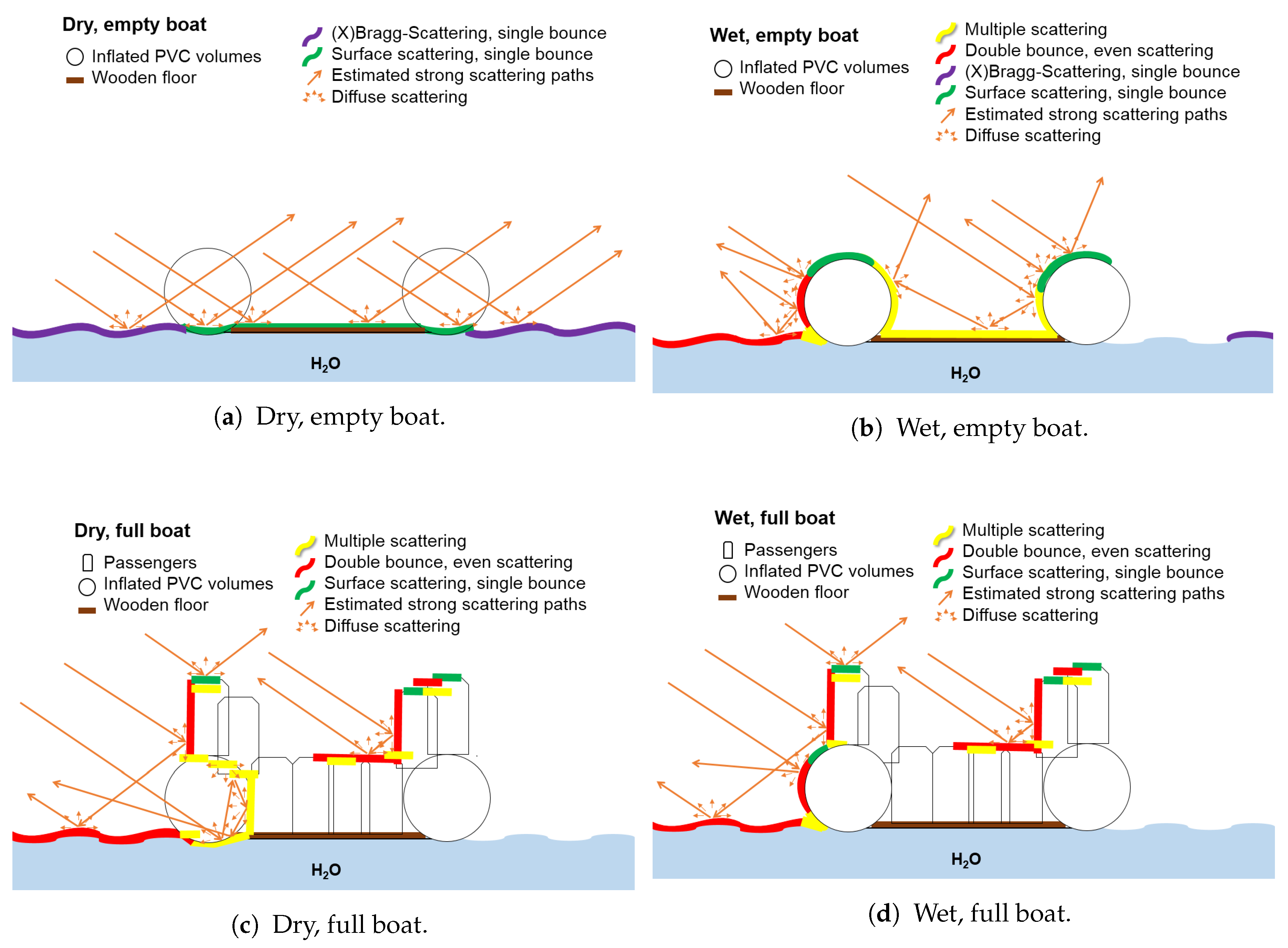
2. A Scattering Model of an Inflatable Refugee Boat

The inflatable vessel used in the InflateSAR experiment is 12 by 3.5 m in size (Figure 1). The volumes rise about half a meter over the water surface. Inflatable of this kind are not ready to cross any bigger water body and they cannot withstand high seas. Therefore, they can be declared as in a state of distress from the moment of disembarkation. The construction materials used were rubber (mainly PVC) and wooden floor plates as stabilizing inlays. Excluding the outboard engine and small rings and bits, there are no metallic components. The small size of the engine and the absence of other large metallic parts results in a small radar cross section. This was expected to impede detection efforts.

When microwaves impinge on a surface, the energy backscattered depends on many physical factors. A very prominent one is the dielectric constant $ϵ$. $ϵ$ is an intrinsic characteristic of the material and varies due to a number of factors, such as the material’s moisture, temperature and salinity. It can be used for the identification of specific materials, for example, metals [74]. Plastic exhibits a low dielectric constant, which makes the material relatively transparent to the radiation in C and X bands. However, the situation changes if the plastic is covered by a thin layer of water (even just a few millimeters, brought about by dew or spray). This is because the dielectric constant of water is very high in C and X bands.

Figure 2 should give an idea about the appearance of the different scattering mechanisms expected on the rubber inflatable. They are shown in an example scenario of low sea state, under an incidence angle of 57${}^{°}$ with the boat broadside facing the sensor’s LoS at 90${}^{°}$. The model shows how in theory the dominant mechanisms change depending on wetness and the presence or absence of passengers. Refraction of the electromagnetic wave is expected when passing through media of different refraction indices n at TerraSAR-X’s carrier bandwidth ($\lambda$ = 9.65 GHz), such as air (n ≈ 1), polyurethane (n ≈ 1.6) and the wooden floor (n ≈ 1.5). The resulting changes of direction before and after the optical thicker mediums are expected to level each other out. Layover shadows prevail at the faces and objects facing away from the sensor. Possible complementary phenomena, such as constructive reflection, destructive reflection, frustrated total internal reflection and the phase jump of $\frac{\lambda }{2}$ as a function of the incidence angle $\varphi$ should be mentioned here but are not addressed in Figure 2. The same is true for the polarization, which also affects the scattered wave.

Another important factor is the target’s and the water surface’s roughness. X-band (TSX) and C-band (S1) radar sensors have very limited penetration in liquid water. Since satellite SAR is side-looking, a flat and calm water surface is particularly smooth and scatters very little energy back to the sensor, which is why it appears black in SAR images; the energy is reflected away in the specular direction, as for a mirror. In most of the cases, water surfaces have waves (e.g., capillary and gravity, swells, etc.). Waves and spray induce surface roughness which produces complex scattering interactions, such as Bragg scattering [75]). The sea state is subject to wind speed and wind direction and always is the combination of wind waves from local winds and swell generated by distant weather systems.

Apart from the scene characteristics, sensor parameters such as wavelength, polarization, incidence angle and radiometric and geometric resolution largely affect the pixel backscattering. These in return influence the capability to detect vessels. In conclusion, a better understanding of scattering mechanisms for water and target connected to scene conditions and system parameters is essential for our undertaking. This is not only for evaluating the detection capabilities, but also for inverse modeling approaches and the design of future data acquisition campaigns.

In terms of polarimetric richness, we can separate data into single, dual and quad (or full) polarization data which respectively include one, two or four polarization channels. Quad-pol data yields better results compared to single-pol or dual-pol data due to its increased information including more independent images, but it suffers from the trade-off a decreased spatial resolution, a smaller swath width or a higher noise level [74,76,77]. Advanced methods based on quad-pol data and polarimetric decomposition methods can be applied. They enable the identification of scattering mechanisms such as surface, volume and double-bounce scattering. The exploration based on different combinations of those add a viable layer of information to ship detection approaches (e.g., [22,69,78,79]).

3. Data

3.1. Data Collection Campaign

In this work we acquired a unique SAR dataset with the ground-truth of a refugee inflatable. Data are from the DLR mission Tandem-X and from ESA’s Sentinel-1. The five-month data collection campaign was implemented in 2017 at the Müggelsee, a lake near Berlin. In this experiment we were concerned with investigating the backscattering from the inflatable with the minimum disturbance possible from the surrounding water surface’s clutter. A lake was selected due to the reduced presence of large waves and absence of breaking waves, spray and sea foam. The backscattering from a small lake was expected to be very low and the radar backscattering produced by the inflatable was meant to be easier to delimit. Further, it allowed us to identify more easily the polarimetric scattering mechanisms occurring at the vessel and to gain a deeper understanding of their influences on the vessel’s radar cross section and the inflatable’s detectability. Ground measurements were accomplished using a standard GPS receiver with an average accuracy of about five meters.

The acquisition campaign was designed to cover a broad variety of the main sensor settings which are polarization, resolution and incidence angle. It resulted in 53 TSX, five TDX (within this paper, they are used and listed as TSX “movingR”) and eight S1 SAR images, collected during 45 data gathering sessions (

Table 1. SAR data collection according to acquisition mode, polarization and incidence angles (low angles “L”, high angles “H”).

Mission	Acquisition Mode	Single pol HH	Single pol VV	Dual cross-pol	Dual co-pol
TerraSAR-X (TSX)	High-Res. Spotlight (HS)	1L, 7H	1L, 4H	n.a.	2L, 12H
	Stripmap (SM)	1L, 4H	1L, 2H	1L, 5H	3L, 9H
TanDEM-X (TDX)	High-Res Spotlight (HS)	1L, 2H	n.a.	n.a.	0L, 2H
Sentinel-1 (S1)	Interferometric Wide Swath (IW)	n.a.	n.a.	2L, 6H	n.a.

). In this study, “low angles” cover incidence angles between 20° and 36°, whereas the category of “high angles“ represents those between 37° and 53°. The nominal spatial resolution varies depending on incidence angle and polarization. The pixel shape and size underwent reconfiguration due to pre-processing, including geocoding where we primarily tried to maintain the spatial resolution. Most HS mode data has around one meter pixel size, for SM mode values vary between one to two meters, and S1 data used for this study reaches about 8.5 m. Some polarization channels, such as full polarized data, were not available. Therefore, the study is limited to co-polarized single (HH, VV) and co/cross-dual polarized (HH+VV, HH+HV, VH+VV, VV+VH) channel combinations.

Table 2. Pixel size in $m^2$ of available acquisition modes after resampling.

	TSX-HS	TSX-SM	S1-IW
Single-pol	0.79	1.52	-
Dual-pol	1.45	2.57	71.74

lists the average pixel size for different acquisition modes in square meters, for which Figure 3 provides a visual overview. The image to the right illustrates the size ratios between the various data’s pixels and the the boat. HS mode and SM mode are assumed to have satisfactory spatial resolution for a successful identification. In S1’s IW mode the pixel area is about two times the vessel’s area, hampering detection efforts. Therefore, it is very likely that S1 data do not reach the minimum resolution needed for a successful identification of our target and more S1 data would be necessary to finally prove this.

During the campaign we covered different combinations of the inflatable’s superstructure (full/empty boat), movement and orientation relative to the sensor’s LoS by six setups called “experiments“ (

Table 3. Data collection: available datasets per experiment type.

Experiment	Movement	Orientation	Superstructure	# Images
				TSX	S1
orthogonal	static	90${}^{°}$	empty	27	8
inclined	static	45${}^{°}$	empty	10	0
parallel	static	0${}^{°}$	empty	4	0
full	static	90${}^{°}$	30 passengers	4	0
movingAZ	moving	90${}^{°}$	empty	8	0
movingR	moving	0${}^{°}$	empty	5	0

). It was the goal of these experiments to examine the impacts of selected scene settings on the boat’s radar backscattering pattern and its detectability. The main ideas behind the experiments’ designs are:

• The superstructures of said open-top inflatables are shaped by the cargo, in our case the passengers. A boat fully loaded with people is expected to change scattering mechanisms (e.g., modeled as adding volume scattering and multiple reflections). To investigate these influences, four data takes had 30 passengers occupying the vessel.
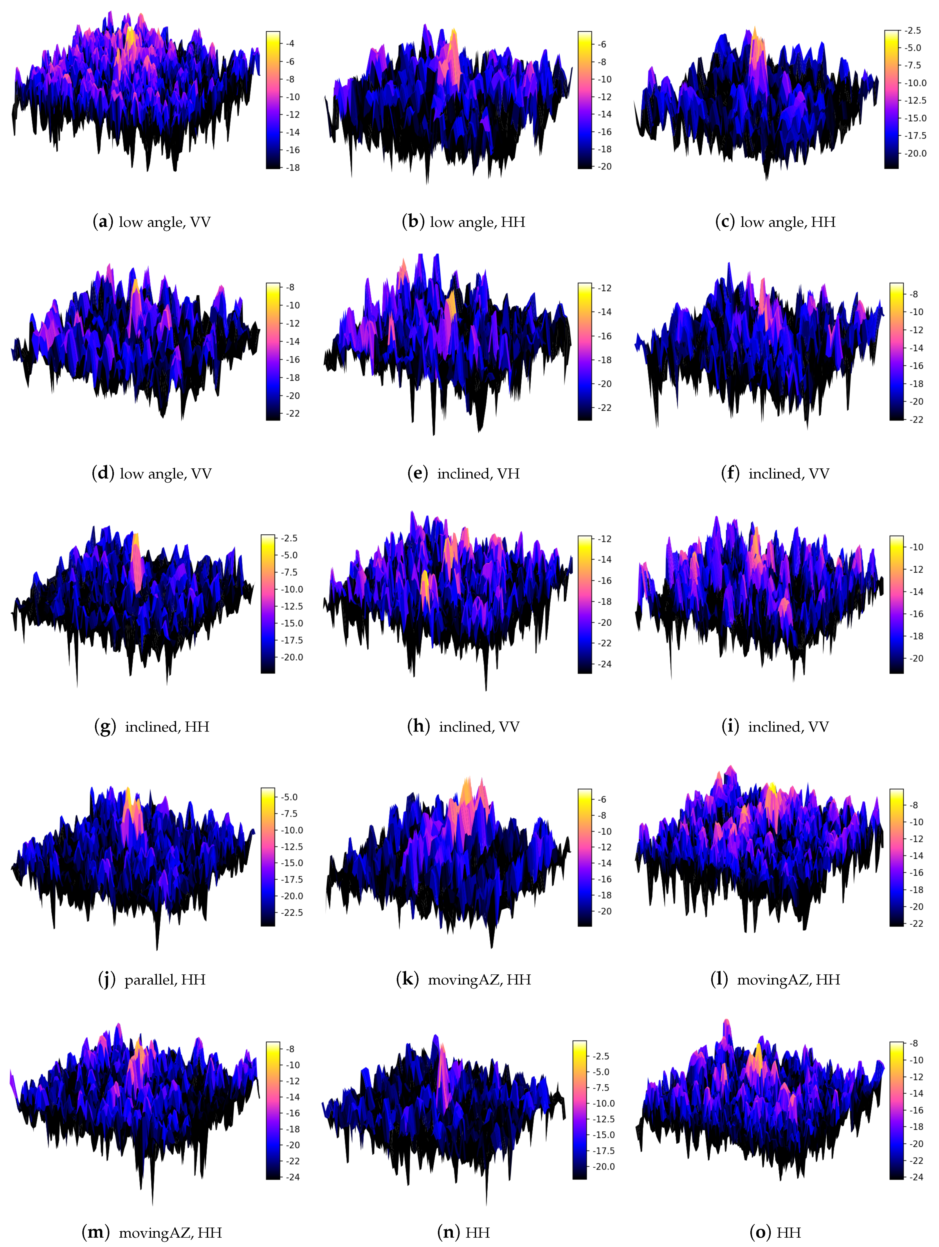
• To test the influence of the inflatable’s orientation compared to the radar wave’s path, the vessel faced different parts toward the sensor: prow or stern side orthogonally (“parallel”), the broadside orthogonally (“orthogonal”) or the broadside at an angle of 45° (“inclined”). This should add to an analysis of the backscattering behavior of specific parts of the boat, such as the outboard engine, double bounce caused by its passengers and double bounce and volume scattering at the broadside or at the prow of the boat. In principle, electromagnetic waves, impinging on the vessel at 45°, are expected to be scattered away, whereas orthogonal or parallel vessel orientation should lead to a situation wherein the backscattering should be higher.
• Two of the experiments include a moving inflatable at its highest possible speed (∼10 km/h), where “movingAZ” has a boat moving in azimuth and “movingR” relates to movement in ground range. Movement is expected to provide the possibility of detecting the position and orientation of its wakes. However, movement involves smearing effects and azimuth displacement which may impede the detection.

Apart from the described sensor and scene settings, the morphology of the data is subject to a number of additional scene settings which are not controllable. Amongst them are the inflatable’s surface humidity and the wind situation. The latter was quite stable throughout most acquisitions (

Table 4. Wind speed and wind direction during the data collection.

(a) Wind speed (ms−1).
	<2.5	2.5–5	5–7.5	7.5–10
# TSX datasets	24	21	6	2
# S1 datasets	6	0	2	0
(b) Wind direction (in degrees relative to the LoS).
	<30${}^{°}$	31–60${}^{°}$	61–90${}^{°}$
# TSX datasets	27	20	6
# S1 datasets	4	2	2

). In the great majority the wind speed is below 5 ms${}^{-1}$ and the prevailing winds were westerly, deviating no more than 30${}^{°}$ from the LoS (Table 4).

The vessel’s surface moisture was recorded during each acquisition, since especially in the morning, chances were good that the volumes of the inflatable were covered by water drops due to rain or dew. In about 60% of attempts the boat could be identified when it was dry compared to 40% in case of wet conditions. The influence of the boat’s moisture on the detection capabilities or its radar backscatter behavior could not be proven statistically, though. For that, a much more comprehensive data basis would be necessary here.

3.2. First Inspection of the Backscattering of Inflatable Boats

The preliminary processing includes radiometric calibration, geometric calibration and georeferencing. Pre-processing steps are slightly different for each satellite platform. For instance, S1 data require additional processing steps, such as applications of an orbit file, removal of thermal noise and debursting. This was done using the Sentinel Application Platform (SNAP) in combination with the Sentinel-1 Toolbox from the European Space Agency.

After the pre-processing, the image pixels represent the normalized radar cross section expressed as scattering coefficient or Sigma Nought ($\sigma$⁰). Speckle filtering or multilooking was tested, but due to the very small size of the boat they reduced the maximum backscattering and decreased its TCR. Therefore, multilooking was not applied to preserve the data’s full spatial resolution at the expense of speckle reduction. Figure 4 shows a part of two of such scenes after pre-processing and projecting into the geodetic reference system WGS84. The corresponding snippets further down are Figure 5g for Figure 4a and Figure 6g for Figure 4b. The lake can be clearly recognized as the dark area with relatively low radar response and bright dots representing buoys and maritime vehicles; amongst them there is our inflatable at the tip of the white arrow. Most of the surroundings are forest with a residential area in the north-east. Figure 4b was taken on a descending orbit with the sensor viewing from the east receiving strong backscatter from the first treeline on the lake’s western shores. The ascending orbit of Figure 4a brightens up the treeline on the eastern shore.

The water surface clutter and the inflatable’s radar signal were statistically analyzed in a consistent way and its backscatter behavior was classified throughout the different datasets. The main purpose was to assess the detection capabilities under different sensors and scene settings. To identify the vessel and to define its extent, we used pixels with noticeably higher intensity values compared to the water surface clutter. All further analyses were computed based on this intensity-based definition of the vessel.

The galleries in Figure 5, Figure 6 and Figure 7 show the intensity ($\sigma$⁰ in dB) of the vessel’s radar pattern of all positive identifications after pre-processing. The 100 by 100 m sized cut-outs center the boat and are grouped by acquisition mode. The colour ramps use each individual image’s mean value as the minimum (dark) and the maximum value for strong radar response. The subtexts indicate the polarization plus one important scene or sensor parameter. Images with no further description were acquired under a “standard” set of parameters: high incidence angle; stationary; empty boat oriented orthogonally to the LoS. That is also true for Figure 8, Figure 9 and Figure 10, below which we come up with the 3D-representations of the same data of $\sigma$⁰ values in dB-scale. Here, each color scale covers the full range of values. They illustrate that the vessel’s radar signatures differ a lot in terms of size and contrast between the images. That challenges any attempt at developing automatic identification techniques.

4. Methods

4.1. Water Surface Clutter

Although the main purpose of this work was the analysis of backscattering from inflatable vessels, in this section we show a clutter analysis to understand its impact on our vessel identification and analysis. In detection theory, the radar backscattering from the water surface is referred to as clutter. In X-band, the water clutter can be very strong, leading to false alarms at all incidence angles [9]. Water clutter depends on wind speed and direction. As already stated above, we selected a small lake as the test site so that the water clutter was less strong. Nevertheless, due to wind conditions, five datasets have strong clutter and an additional five show moderate clutter. We defined the clutter level through the degree of inhomogeneity of the whole lake surface’s radar response. The dispersion is a suitable value to measure, since it combines the influences of the clutter’s standard variation (${\sigma }_{clutter}$) and the clutter’s mean values (${\mu }_{clutter}$).

$$Dispersio{n}_{clutter}=\frac{{\sigma }_{clutter}\times {\sigma }_{clutter}}{{\mu }_{clutter}}$$

(1)

The higher the ${\sigma }_{clutter}$ normalized by ${\mu }_{clutter}$, the less homogeneous the water is in the radar image. Here, images with a dispersion value smaller than two are classified as having weak clutter levels, greater than two are moderately cluttered and those with a dispersion greater than three are defined as strongly cluttered. This convention corresponds well to the results of the visual image interpretation.

Wind speed and wind direction do trigger higher levels of water surface clutter that can be modeled using Bragg scattering ([80,81]). Thanks to the friendly support of the Leibnitz-Institute of Freshwater Ecology and Inland Fisheries (IGB), in situ weather data from the nearby observation station “Georg Mothes” at 52${}^{°}$26${}^{\prime }$46.3${}^{″}$ N 13${}^{°}$38${}^{\prime }$60.0${}^{″}$ E were available for each acquisition.

Figure 11 compares wind speed and wind direction (the absolute difference to the sensor’s LoS in degrees) with the water surface’s clutter strength and acquisition mode. Eight out of the ten acquisitions showing “moderate” or “strong” clutter were collected when the wind direction was less than 30° with respect to LoS. This produces waves moving mostly parallel to the LoS, which could contribute to a stronger clutter response. Higher wind speed especially increases the chance of moderate or strong clutter throughout the collected datasets.

Figure 12 examines the radar response of the 250 × 250 m sections of the surrounding water area with the boat in the center. Low maxima and low dispersion values benefit a higher TCR and better identification capabilities (bottom left areas). We labeled datasets finding themselves in the upper right corner as biased by strong clutter.

This label was taken into account for some of the following analyses. Cross-polarized data deliver low dispersion values (low heterogeneity) from the water surface and at the same time a very low maximum $\sigma$⁰. Low incidence angles are more affected by strong clutter and have high clutter dispersion. Data acquired with a high incidence angle have lower water surface clutter and seem more promising for better identification capabilities. The water surface in S1 data reach on average lower mean and maximum $\sigma$⁰ by about 5 dB compared to TSX data. Images which are marked as affected by strong clutter are characterized by higher mean values (TSX: +7 dB, S1: +5 dB) and a higher clutter maximum (+10 dB). In view of designing an automatic ship detector, it could be appropriate to adopt multilooking and to apply different processing methodologies when the clutter is particularly strong.

4.2. Identification Scheme

This work was focused on analyzing the backscattering behavior of inflatable vessels. The following methodology is heavily supervised and it is not proposed as an operational technique. We used it here for the mere purpose of identifying the vessel pixel for the statistical analysis. The inflatable identification approach uses intensity values and therefore follows the principles of a simple intensity-based detector with adaptive thresholding. We calculated the TCR as the difference (in dB) between the vessel’s maximum backscatter and ${\mu }_{clutter}$ where ${\mu }_{clutter}$ is a representative of the clutter intensity in dB for the lake’s backscattering in each acquisition:

$$TCR=maximu{m}_{vessel}-{\mu }_{clutter}$$

(2)

To apply adaptive thresholding to our visual identification scheme, we compared the boat’s maximum intensity value with the respective scene’s clutter dispersion by using the clutter’s mean and standard deviation. Visual identifications are labeled reliable if:

$$maximu{m}_{vessel}>{\mu }_{clutter}+3\times {\sigma }_{clutter}$$

(3)

The selection of factor 3 in Equation (3) is a crucial decision which influences all further results. According to literature, a TCR of at least 10 dB is acknowledged as being reasonable for reliable detection and identification with automatic vessel detection systems [82]. Since all ${\sigma }_{clutter}$ in our data are between 3.2 and 5.9, using three times ${\sigma }_{clutter}$ will lead us to thresholding similarly to the one suggested.

Additionally, an automatic blob detection algorithm was implemented using Python and OpenCV. The blob detector had limited success due to different clutter levels throughout the data. This shows the importance of adaptive thresholds, even in such a homogeneous test bed as in our case. Please note that these algorithms were supervised and were used only for providing a good delineation of the vessel for the analysis of its backscattering. In the future, more work needs to be carried out ifor finding an automatic detection methodology.

Our classification scheme enabled the analysis of the inflatable radar backscatter. Figure 13 illustrates two very different scenarios in false colors where dark blue pixels represent intensities smaller than ${\mu }_{clutter}$. All other colors have values bigger than ${\mu }_{clutter}$ with a class width of the standard deviation ${\sigma }_{clutter}$. The inflatable in Figure 13a has a comparatively low TCR since most of the pixels representing the vessel show intensity values similar to the some parts of the quite heterogeneous surrounding sea clutter. In Figure 13b the boat has a clearly higher intensity than the water surface, making this case more favorable for vessel identification. Moreover, the surroundings are of favorably low dispersion. Wind speed and direction relative to the line of sight are influencing the water surface’s radar response. In big water bodies the swell adds to the local sea state. Very calm water leads to low or null surface scattering. In general, bigger waves produce stronger radar backscattering. In our dataset, we observed different wind conditions. Since this was a lake, trees were also sheltering some water areas with some wind directions. This explains the variability of water clutter in the images that we acquired.

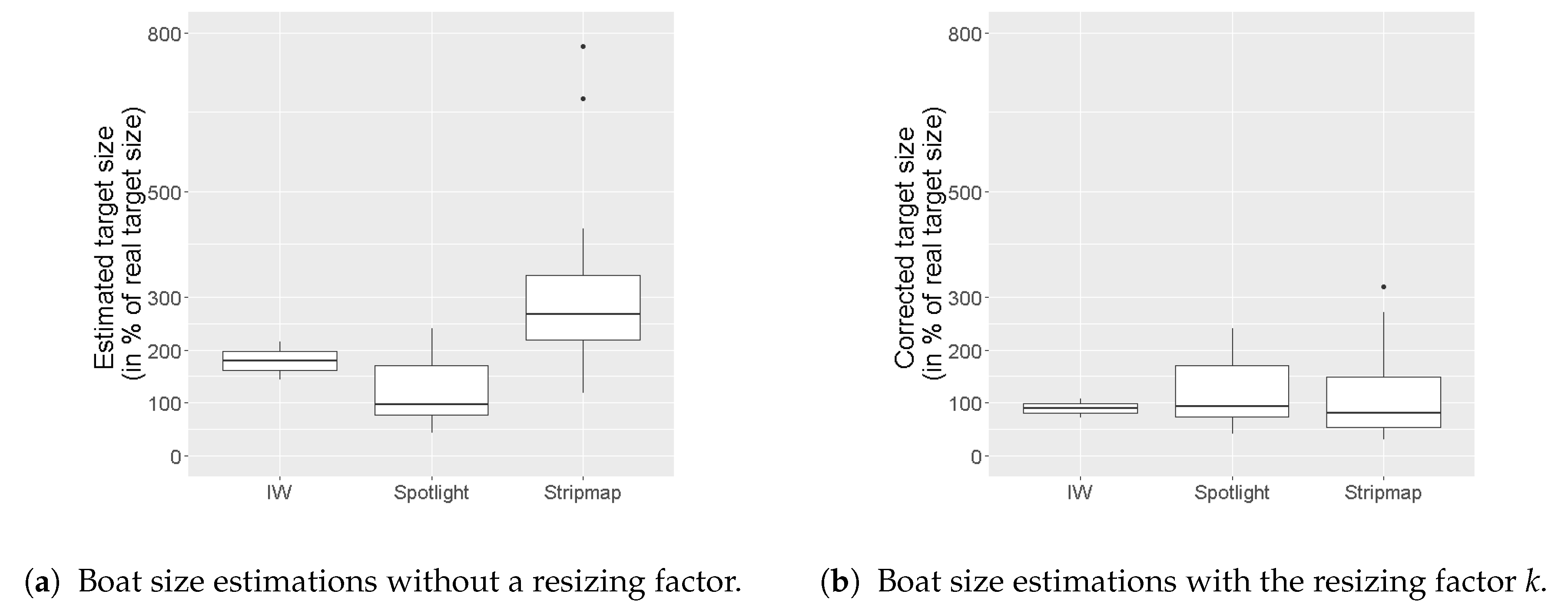
4.3. Estimation of the Inflatable’s Size

When assessing the capability to successfully identify a target, we can use both maximum TCR and detected size, because larger targets are easier to detect than smaller ones. Moreover, exact estimation of the detected inflatable’s size enables us to discriminate it from other marine objects. This is especially true for the open sea far off the coast, where marine vehicles of such small dimensions are rather unlikely, since the great majority of marine traffic consists of much larger vessels (>100 m in length and at least several meters of freeboard).

We estimate the boat size by multiplying the number of pixels assigned to the vessel category by the pixel area. Figure 14 shows the results in a box and whisker plot with the lower and upper hinges corresponding to the first and third quartiles and the whiskers extending from the hinges to the largest value no further than 1.5 times the inter-quartile range. TSX’s HS mode delivers quite good results with an average of 93% of the real boat size (Figure 14a). However, with the spatial resolution going down, the results deteriorate and the comparatively coarse spatial resolutions of TSX’s SM mode and S1’s IW mode are not suitable for that simple approach.

In order to produce more accurate estimations of the vessel silhouette, we can adjust the edges by using what is sometimes called spatial hysteresis. This exploits vicinity conditions [83]. Here, we used a scheme where we split boat’s radar signature into two groups. The first group are high intensity pixels (intensity > $\mu$ + 3*$\sigma$) and we assigned them to the category $are{a}_{vessel}$; the second group are the adjacent, lower-valued pixels ($\mu$ + 3*$\sigma$ > intensity > $\mu$ + 2*$\sigma$), associated with the category $are{a}_{ambit}$ (Equation (4a)). This gives us the opportunity to apply the now introduced resizing factor k to parts of the estimation formulas. For our TSX SM mode data, we set k = 10 and for S1 data to k = 2 and applied it for SM mode data to $are{a}_{ambit}$ (Equation (4b)) and for IW mode to both, $are{a}_{vessel}$ and $are{a}_{ambit}$ (Equation (4c)):

$$siz{e}_{vessel}^{HS}=are{a}_{vessel}^{HS}+are{a}_{ambit}^{HS}$$

(4a)

$$siz{e}_{vessel}^{SM}=are{a}_{vessel}^{SM}+\frac{are{a}_{ambit}^{SM}}{k^{SM}}$$

(4b)

$$siz{e}_{vessel}^{IW}=\frac{are{a}_{vessel}^{IW}+are{a}_{ambit}^{IW}}{k^{IW}}$$

(4c)

The results of that correction of the initial size estimations are plotted in Figure 14b. It can be seen that the corrected estimations are much more accurate, but since the values for k deviate from our data, they need to undergo testing and assessment with alternative data.

5. Results

5.1. Analysis of the Inflatable’s Backscattering

Before delving into the analysis of the backscattering with regard to sensors and scene parameters, here we want to present a table summarizing the capability of seeing the inflatable in the SAR image. This visibility test is at the base of all the other analyses and provides an overview that could inform possible future data acquisitions.

Table 5. Identification rate according to scene and sensor parameters: positive identification in % (datasets available, which suffer from increased clutter).

		Experiment						Sum (only TSX)
		Orthogonal	Inclined	Parallel	Full	MovingAZ	MovingR
Polarization	HH	83 (12;4)	75 (4;0)	100 (3;1)	100 (3;0)	100 (5;1)	0 (4;1)	77 (31;7)
	VV	83 (12;3)	100 (4;1)	100 (1;0)	100 (1;0)	50 (2;0)	0 (1;0)	81 (21;4)
	HV/VH	0 (3;0)	50 (2;0)	-	-	0 (1;0)	-	17 (6;0)
Incidence Angle	high	88 (17;0)	80 (10;1)	100 (4;1)	100 (4;0)	75 (8;1)	0 (4;0)	79 (47;3)
	low	50 (10;7)	-	-	-	-	0 (1;1)	45 (11;8)
Platform/ Acquisition Mode	TSX-HS	77 (13;4)	100 (3;1)	100 (3;1)	100 (4;0)	75 (4;0)	0 (5;1)	72 (32;7)
	TSX-SM	71 (14;3)	71 (7;0)	100 (1;0)	-	75 (4;1)	-	73 (26;4)
	S1-IW	25 (8;1)	-	-	-	-	-	25 (8;1)
Sum (only TSX)		74 (27;7)	80 (10;1)	100 (4;1)	100 (4;0)	75 (8;1)	0 (5;1)	72 (58;11)

shows the probability of identification in our data collection. The figures in brackets indicate the number of datasets available and the number of which suffer from stronger clutter. The overall rates of true positive identifications reached 72% for TSX and 25% for S1. Some of the sensor parameters (rows-wise) turned out to have impacts on the detection probability: cross-polarized data clearly cause difficulties identifying the inflatable boat with the lowest sensor-bound rate of only 17%. That shows that the boat does not depolarize the wave and it is likely that single or horizontal double bounce scattering mechanisms may be in place.

It seems that low incidence angles are more likely to be affected by strong clutter, which decreases the TCR and the chance of identification compared to high angles. Eight out of eleven low-angle images have strong clutter, reducing the identification rate to only 45%. On the contrast, low incidence angles with moderate clutter signature are highly suitable for identifying the inflatable with a rate of 100%. The rather flat superstructure of the vessel and its small height do not expose much area to the incoming radiation. This leaves double bounce scattering at the broadside of the vessel not adding to the radar response as strongly as is usually expected in ship detection. That could hamper the identification capability for all cases, but especially for higher incidence angles. To prove that assumption, we need more data of that category without strong clutter.

TSX’s HS and SM modes show much higher identification rates than S1’s IW mode, since IW mode’s spatial resolution is much lower. As a consequence, the energy of the vessel’s radar backscattering is spread over a larger area, reducing its normalized cross section. This reduces the TCR and makes the identification of the boat impossible for most cases.

The scene parameters are listed as columns and do add some influences in this context as well. If we only looked at images with moderate clutter, the category orthogonal would reach 100%. That setup, when the stationary boat is oriented at 90° to the LoS, delivers the best results, as expected. This is because the boat faces the radar, exposing the biggest side at a 90° orientation, and it is expected to produce more single and double reflections. High detection rates are achieved as well for stationary vessels oriented in a parallel way (parallel) to the LoS and for stationary vessels carrying 30 passengers (full; oriented at 90°). The parallel case also supports the occurrence of single and double bounce mechanisms at the front where the bow rises from the water and at the counter stern. A full boat rises about twice as high from the water’s surface due to the passengers sitting on top of the inflatable volumes, triggering stronger multiple reflections.

Reduced identification capabilities are observed if the stationary vessel is orientated 45${}^{°}$ to the LoS (inclined), since the faces are oriented in a way that would reflect the energy away from the sensor. Having an inflatable moving in azimuth direction (movingAZ) at a maximum speed of about 10 km/h produces a smearing effect and reduces the TCR. We expect this to decrease the chance of identification. MovingR represents interferometric TDX-acquisitions with an inflatable moving in range which brings about azimuth displacement. We do not expect the misplacement to have a large impact due to the moderate velocity and the quasi-real time nature of the detection. However, defocusing could impede identification. Since we did not apply interferometric techniques up to now, a secure identification with MovingR-TDX-data was not possible.

Summing up, the main reasons for an unsuccessful identification seem to be a combination of at least two of the following factors: an inclined or a moving vessel, cross-polarization, a low incidence angle and a coarse spatial resolution. When removing the movingR experiments from the statistics, co-polarized data and high incidence angle data reach the best identification rate of about 86%.

5.2. Assessment of Acquisition Parameters

In Figure 15 we show the quality of all 44 positive identifications using the indicators TCR (intensity values in terms of $\mu$) and corrected vessel size estimation (Section 4.3 introduced the resizing factor k applied). The most favorable results have high TCRs while being located near the 100% line. The data were divided into five experiments representing different scene settings (boat orientation, superstructure/cargo and movement).

To take a closer look at differences in the quality of identification between horizontal and vertical polarization we used dual co-polarized datasets (HH+VV). This allows a fair comparison of polarization channels because all other sensors and scene parameters are equal for each pair of acquisitions. Figure 16a lists representations of dual-pol datasets along the x-axis, where seven out of eight cases show larger over-estimations of the boat size with the horizontal polarization channel. The TCRs (Figure 16b) are of comparable quality for HH and VV. Therefore, there is no ground to give a clear preference for either of the two polarization channels. For completeness, Figure 16a shows dual-pol datasets where only one image allowed for a successful identification too.

5.3. Analysis of Clutter Effects

Beside the scene and the sensor settings, the vessel identification throughout the experiments is subject to a number of uncontrollable influencing factors, such as clutter. In general, a higher water surface response decreases the TCR. For our data we define the clutter with intensity (${\sigma }^0$) values up to the “maximum clutter” level of the median ($\mu$) plus two times the standard deviation ($\sigma$). Intensities above that threshold are assumed as coming from other objects than the water’s surface. We try to explain strong clutter with a high $\mu$ (strong water surface response) and a high $\sigma$ (high inhomogeneity).

Figure 17 searches for impacts of the sensor and scene settings on the TCR before the background of a statistical analysis of the surrounding water surface’s clutter. Figure 17a,b show the sensor settings, whereas Figure 17c,d focus on the scene settings. In Figure 17b,d we applied the standard deviation of the ${\sigma }^0$-values to the x-axis, and for Figure 17a,c the maximum clutter thresholds were used. Unsuccessful identifications are represented with TCRs of zero. With the background color we illustrate the idea that chances of a reliable vessel identification can be estimated with TCRs relative to the surrounding water surface’s clutter behavior—here near or greater than $\mu$ plus three times $\sigma$, a condition represented by the green area. True positive identifications within the white-reddish area should be flagged with a lower reliability.

The figures show that SM mode tends to have slightly lower values for maximum clutter and standard deviation compared to HS mode, which is favorable for vessel identification. Clutter from the S1 mission stands out with higher $\sigma$s, lower $\mu$s and lower TCRs. The figures support the above statement that cross-polarization and low incidence angles decrease identification capabilities. Further, a vessel full of people is more visible in our data, whereas having the boat oriented at 45${}^{°}$ to the LoS or moving in azimuth decreases the TCR.

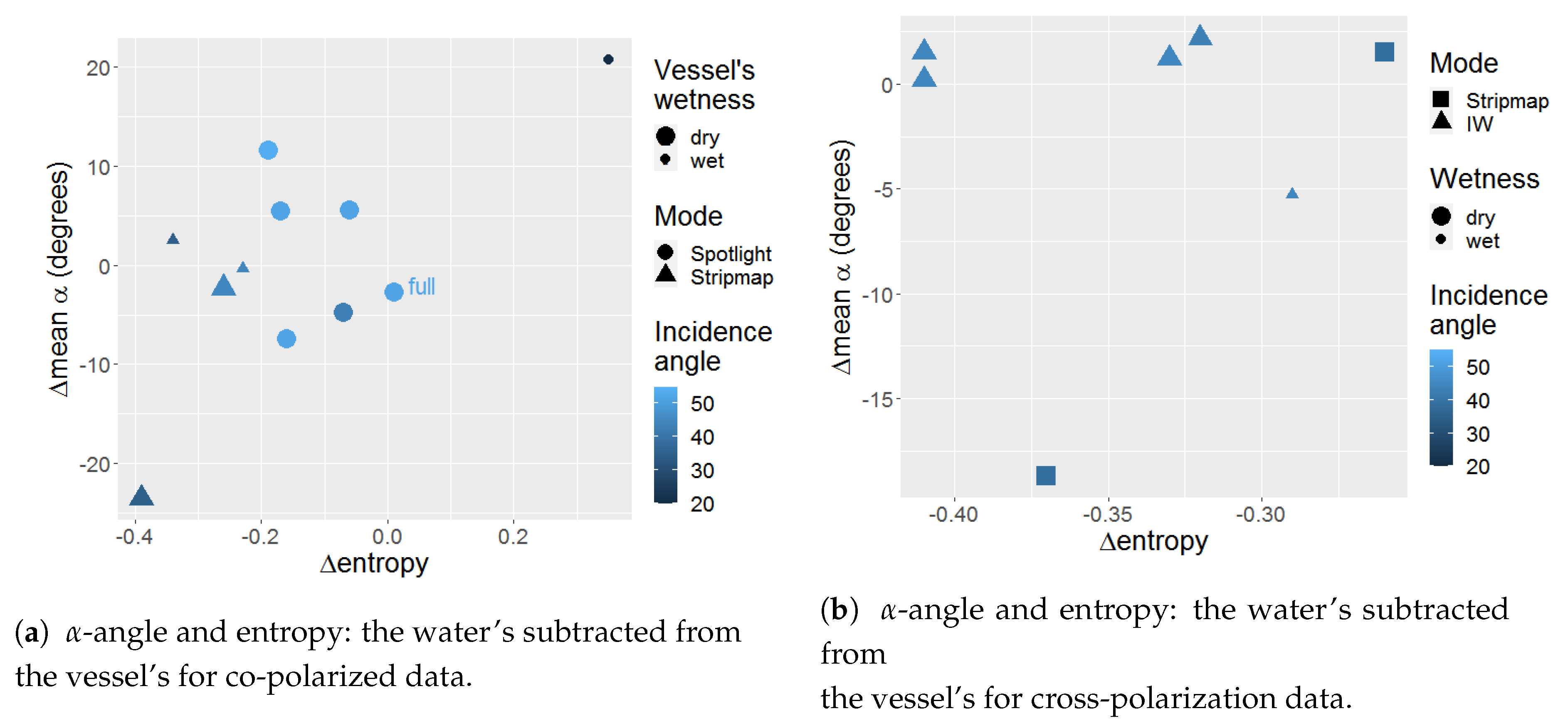
5.4. Polarimetric Analysis

When dual-pol HH/VV images were available, we carried out a polarimetric analysis using the Cloude Pottier decomposition. The polarimetric interpretation of the entropy/alpha (H/$\alpha$) space could be done, since with HH/VV polarization channels we can change the coordinate system to the Pauli one and the eigenvectors can be interpreted as in the quad-pol decomposition.

The comparison between the vessel and the water’s surface shows clear differences regarding the polarimetric behavior: the results for the boat (Figure 18a,c) reveal a preference for dipole and cylinder scattering, with entropy that can be relatively low. This is quite uncommon for ordinary ship identification, where the entropy is generally high. This is due to the limited size and number of structures over this inflatable vessel. The water surface (Figure 18b,d) presents relatively high values of entropy with an $\alpha$ that sits around 50°. This is a sign that the clutter backscattering is close to the noise floor.

Figure 18c,d show the scene settings. It can be observed that a vessel being full or moving in azimuth has higher entropy. For our data, the characteristics of dominant scattering mechanisms depend on vessel orientation and superstructure. The weather conditions at the moment of acquisition were recorded as well. In Figure 18c wet indicates drops of water or a thin water layer on the surface of the inflatable’s volumes, either from rain or dew. Apart from the tendency that wet inflatables have rather low entropy, there is no explicit connection between the boat’s polarimetric parameters and its wetness. A clear pattern of the influence of the wind conditions could not be observed. Adding the sensor settings to Figure PolSensorSetta,b might lead to the assumption that a low incidence angle sometimes drastically reduces both the water’s and the boat’s entropy and the mean alpha angle.

For completeness, Figure 19a–d shows the H/$\alpha$ space for cross-polarization data. A physical interpretation here is not straightforward, nevertheless the decomposition can be used a signal processing tool to show that the backscatter behavior of the boat and the water are different.

Figure 20 now compares the previous results and embraces the vessel’s particular behavior in the H/$\alpha$-space compared with the surrounding water surface. Additionally, selected sensor and scene settings were added to the plot to leave more room for interpretation. Co-pol (Figure 20a) and cross-polarization (Figure 20b) scenarios show that the entropy can be used to discriminate between the two entities, as the vessel has lower values in all acquisitions, except for one case, in Figure 20a. The limited amount of data does not support a sound assessment, but the very low incidence angle and the vessel being wet could have made a difference. The $\alpha$-angle does not seem to be useful at all to differentiate the boat from the water body, since divergences do not show a uniform trend. We labeled the one available dataset with a full boat in Figure 20a, since we wanted to especially emphasize the most realistic scenario. The H/$\alpha$-spaces change with increasing wave heights; these results relate to rather calm sea states.

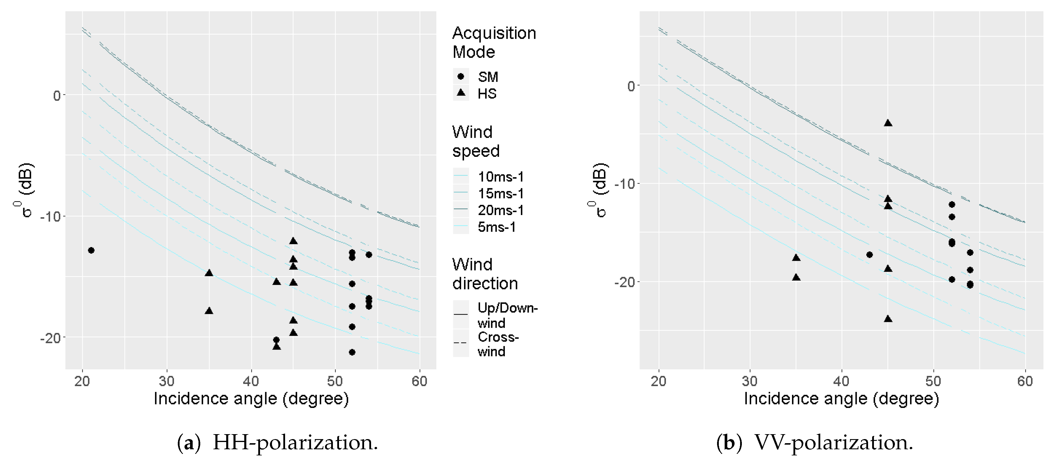
5.5. Emulating the Detectability at Higher Sea States

We want to emphasize once more that the collected data originates from a lake. The findings related to water scattering can only be translated to the real situation in which the refugee vessels are in the open ocean at relatively calm sea states. To estimate the robustness of the identification capabilities, the weather and wave conditions of such an environment has to be addressed. It can be assumed that there are stronger winds and rougher sea states most of the time.

Therefore, we want to bridge the gap with open ocean data and provide an estimation of feasibility for intensity-based identification methods in stronger wind conditions. To do this we used the XMOD1 geophysical model function from [84] to estimate $\sigma$⁰ from U₁₀ wind speed for different wind directions relative to the LoS (cross-wind, up/down-wind) and for a range of incidence angles (20${}^{°}$–60${}^{°}$). Wind speed estimations span the Beaufort scale from 4 (moderate breeze) to 8 (fresh gale) covering a wide range of frequently occurring scenarios of winds in the central Mediterranean capable of bringing severe problems to small refugee vessels.

Figure 21b shows the results for VV-polarization of an X-band radar sensor. To transfer these results to HH-polarization (Figure 21a), we used the polarization ratio model from [85]. The dots represent three times the respective image’s standard deviation subtracted from the maximum radar response from all successfully identified vessels to ensure a decent TCR. The lines represent the estimated intensities of the water surface’s radar response according to different wind scenarios. All phenomenons are drawn with respect to incidence angle and polarization.

6. Discussion

Looking at the high identification rates of our inflatable in this study, we have to bear in mind that the data came from a test site which was designed to ease intensity-based identification. On the other hand, most of our dataset shows an empty boat and our analyses revealed that a fully occupied boat has a stronger radar return (and therefore a better TCR). In a maritime context, our results can only be transferred to a very calm, open ocean with low wind (less than 5 m/s) and no swell. Nevertheless, our findings about the backscattering behavior of small inflatable vessels do represent a basis for further fruitful research in this field. The experiments to test the influences of different scene settings and the polarimetric modes revealed valuable information for further research.

Our preliminary hypothesis of expecting the “wetness” of the boat’s volumes to have influence on both its detectability and its polarimetric signature could not be proven at this stage.

We examined data from different platforms and acquisition modes to evaluate the effects of resolution. It is known that for the current satellites, the higher the spatial resolution, the smaller the areas that can be monitored per unit of time. In addition to this, adding polarimetric channels decreases the image’s spatial footprint. It turned out that dual-pol Spotlight mode data are well usable to identify our special target, whereas Sentinel-1’s Interferometric Wide Swath mode seems not to meet the requirements. However, the use of more sophisticated detection algorithms may make the use of Sentinel-1 feasible in the future.

For the future, it is vital to collect more data using different resolutions (e.g., RadarSAT-2) and with different sea states in the open ocean. Test data or simulations of a fully occupied inflatable would be very valuable to further converge towards the realistic scenario.

7. Conclusions

This article presented an analysis of the very first effective SAR data collection of a refugee inflatable. It proves that using TerraSAR-X, the inflatable boats can be detected with high certainty, despite their low dielectric constant and small size. This was true for the relatively calm weather conditions (mostly less than 5 m/s) and water state prevailing at the test site. Simulations to get a preview how this goal can be achieved in the maritime environment revealed the following:

• Higher incidence angles increase the detectability, since the sea has a lower backscattering, whereas the target signal’s intensity remains relatively stable.
• Wind speed greater than 10 ms${}^{-1}$ dramatically reduces the detectability for most cases. That is true for both HH and VV polarizations.
• Above 15 ms${}^{-1}$, in almost all cases the TCRs get too low to ensure a reliable intensity-based identification.

Unsuccessful vessel identification is in most cases caused by strong clutter. Moreover, specific sensor and scene settings influence the quality of identification to a great extent, such as the vessel’s movement and its orientation compared to the radar path. We observed that:

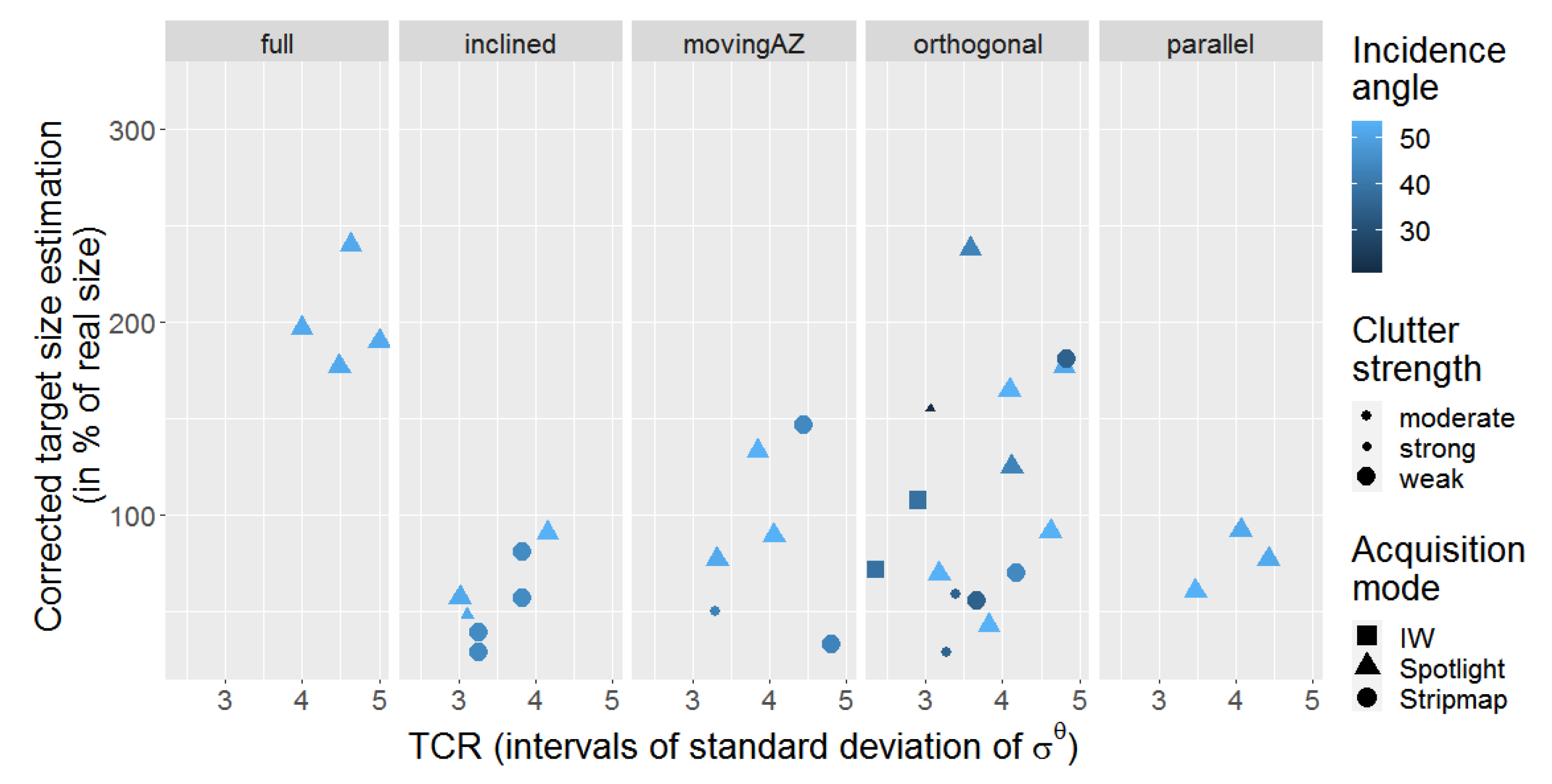
• A full vessel has comparatively larger footprint estimations of around 200% and strong target to clutter ratios between four and five times the standard deviation of $\sigma$⁰. This category can be seen as a reference group, since it represents the most realistic situation.
• Movement in azimuth triggers a smaller TCR due to the well-known smearing effect. The consequence is a reduced identification capability. Size estimations are well around the 100% mark.
• Throughout the experiments, inclined and parallel, the size of the vessel was underestimated and the target to clutter ratios had a tendency to be very low.
• The experiments with a stationary vessel orthogonally oriented (“orthogonal”) led to a quite variable identification quality with boat size estimations mainly between 50% and 150% of the real size and acceptable target to clutter ratios, mostly concentrated in between three and four times of the respective image’s standard deviation.
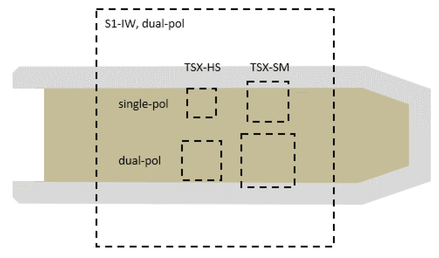
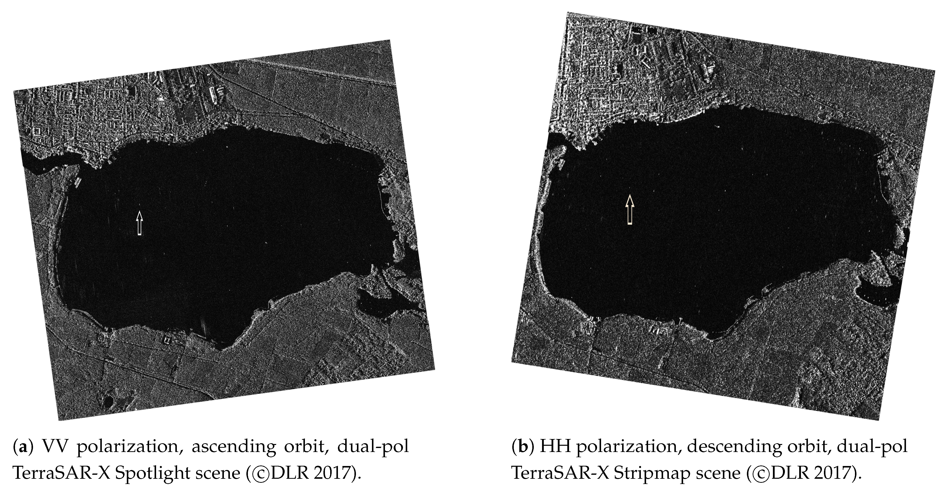
• The acquisition mode played a role with Sentinel-1’s Interferometric Wide Swath mode characterized by very low target to clutter ratios. TerraSAR-X’s Stripmap and Spotlight modes show similar quality of identification throughout. However, this is driven by a combination of many influencing factors and we cannot come to any conclusion without collecting more data.
• The incidence angle does not seem to play a role, but we cannot draw any meaningful conclusions considering the limited availability of low incidence angle data not affected by stronger clutter. However, it clearly is prone to the occurrence of increased clutter, which lowers the TCR due to a stronger radar response from the water’s surface. Chances for automatic identifications for those cases are expected to be lower.
• The majority of corrected boat size estimations are between 50% and 150% of the real vessel size.

In terms of polarization, co-polarized data allow for better object identification than cross-polarized data. Low incidence angles tend to be more susceptible to strong clutter, decreasing the TCR and the quality of identification. The spatial resolution of TerraSAR-X’s Stripmap and Spotlight modes seems sufficient, whereas Sentinel-1’s Interferometric Wide Swath mode provides very low identification rates.

Most of these findings relate to intensity-based identification and detection schemes which may not be applicable to higher sea states in the open ocean. The polarimetric analysis shows that neither the vessel’s superstructure nor its orientation seem to influence its bearing in the entropy-$\alpha$-space much. More importantly, we found that a clear distinction between the vessel and the water surface is possible, which invites the development of polarimetric-based detectors.

The findings of our work show that SAR can be used for a satellite-based surveillance infrastructure to (semi-)automatically identify small rubber inflatables, such as our test vessel in a test bed like a small lake. The establishment of infrastructure like that could considerably support search and rescue missions in the Mediterranean Sea, reduce the number of such boats being missed and mitigate the ongoing death in the open ocean. For that, further research will aim at the comparisons and testing of different detectors, and the development of specially tailored detectors. For validation it is crucial to acquire more test data from the open ocean or to alternatively bridge the gap with a data simulation approach.

References

1. Vachon, P.W. Ship Detection in Synthetic Aperture Radar Imagery. In Proceedings of the OceanSAR 2006—Third Workshop on Coastal and Marine Applications of SAR, St. John’s, NL, Canada, 23–25 October 2006; pp. 1–10. [Google Scholar]
2. Crisp, D.J.; Redding, N.J. Ship Detection in Synthetic Aperture Radar Imagery. In Proceedings of the 12th Australasian Remote Sensing and Photogrammetry Conference, Fremantle, Australia, 18–22 October 2004; p. 10. [Google Scholar]
3. Hannevik, T.N. Evaluation of Radarsat-2 for Ship Detection. Forsv. Forsk. FFI-Rapp. 2011, 1692. Available online: https://ffi-publikasjoner.archive.knowledgearc.net/handle/20.500.12242/1317 (accessed on 22 October 2020).
4. Velotto, D.; Tings, B.; Bentes, C. Comparison of Ship Detectability between TerraSAR-X and Sentinel-1. In Proceedings of the 2017 IEEE 3rd International Forum on IEEEResearch and Technologies for Society and Industry (RTSI), Modena, Italy, 11–13 September 2017; pp. 1–5. [Google Scholar]
5. Fernandez Arguedas, V.; Velotto, D.; Tings, B.; Greidanus, H.; Bentes, C. Ship Classification in High and Very High Resolution Satellite SAR Imagery. In Proceedings of the Security Research Conference, 11th Future Security, Berlin, Germany, 4–6 September 2016; pp. 347–354. [Google Scholar]
6. Marino, A.; Sanjuan-Ferrer, M.J.; Hajnsek, I.; Ouchi, K. Ship Detection with Spectral Analysis of Synthetic Aperture Radar: A Comparison of New and Well-Known Algorithms. Remote Sens. 2015, 7, 5416–5439. [Google Scholar] [CrossRef]
7. Song, S.; Yang, J. Ship Detection in Polarimetric SAR Images via Tensor Robust Principle Component Analysis. In Proceedings of the 2015 IEEE International Geoscience and Remote Sensing Symposium (IGARSS), Milan, Italy, 26–31 July 2015; pp. 3152–3155. [Google Scholar] [CrossRef]
8. Marino, A.; Hajnsek, I. Statistical Tests for a Ship Detector Based on the Polarimetric Notch Filter. Geosci. Remote Sens. IEEE Trans. 2015, 53, 4578–4595. [Google Scholar] [CrossRef] [Green Version]
9. Velotto, D.; Nunziata, F.; Migliaccio, M.; Lehner, S. Dual-Polarimetric Terrasar-x SAR Data for Target at Sea Observation. Geosci. Remote Sens. Lett. IEEE 2013, 10, 1114–1118. [Google Scholar] [CrossRef]
10. Sanjuan-Ferrer, M.J.; Hajnsek, I.; Papathanassiou, K.P.; Moreira, A. A New Detection Algorithm for Coherent Scatterers in SAR Data. IEEE Trans. Geosci. Remote Sens. 2015, 53, 6293–6307. [Google Scholar] [CrossRef]
11. Renga, A.; Daniela Graziano, M.; Moccia, A.; D’Errico, M. Adaptive Threshold and Sub-Look Processing in Ship Detection by SAR. In Proceedings of the OCEANS 2015-Genova, Genoa, Italy, 18–21 May 2015; pp. 1–8. [Google Scholar] [CrossRef]
12. Tian, M.; Yang, Z.; Duan, C.; Liao, G.; Liu, Y.; Wang, C.; Huang, P. A Method for Active Marine Target Detection Based on Complex Interferometric Dissimilarity in Dual-Channel ATI-SAR Systems. IEEE Trans. Geosci. Remote Sens. 2020, 58, 251–267. [Google Scholar] [CrossRef]
13. Gao, G.; Huang, K.; Gao, S.; He, J.; Zhang, X. Ship Detection Based on Oceanic Displaced Phase Center Antenna Technique in Along-Track Interferometric SAR. IEEE J. Sel. Top. Appl. Earth Obs. Remote Sens. 2019, 12, 788–802. [Google Scholar] [CrossRef]
14. Baumgartner, S.V.; Krieger, G. Ship Detection and Motion Parameter Estimation with TanDEM-X in Large along-Track Baseline Configuration. ESA Spec. Publ. 2013, 709, 18. [Google Scholar]
15. Makhoul, E.; Baumgartner, S.V.; Jager, M.; Broquetas, A. Multichannel SAR-GMTI in Maritime Scenarios With F-SAR and TerraSAR-X Sensors. IEEE J. Sel. Top. Appl. Earth Obs. Remote Sens. 2015, 8, 5052–5067. [Google Scholar] [CrossRef] [Green Version]
16. Oveis, A.H.; Sebt, M.A. Dictionary-Based Principal Component Analysis for Ground Moving Target Indication by Synthetic Aperture Radar. IEEE Geosci. Remote Sens. Lett. 2017, 14, 1594–1598. [Google Scholar] [CrossRef]
17. Lombardo, P.; Pastina, D.; Turin, F. Ground Moving Target Detection Based on MIMO SAR Systems. IEEE J. Sel. Top. Appl. Earth Obs. Remote Sens. 2015, 8, 5081–5095. [Google Scholar] [CrossRef]
18. Börner, T.; Marull Paretas, G.; Baumgartner, S.; Lopez-Dekker, P.; Sauer, S.; Krieger, G.; D’Addio, S. ATI and GMTI Performance Analysis of Post-Sentinel-1 SAR Systems Based on Simulations Using OASIS. In Proceedings of the EUSAR 2014 10th European Conference on Synthetic Aperture Radar, Berlin, Germany, 3–5 June 2014; pp. 1–4. [Google Scholar]
19. Margarit, G.; Tabasco, A. European Commission: CORDIS: Projects and Results: Final Report Summary-SAGRES (Services Activations for GRowing Eurosur’s Success). Available online: https://cordis.europa.eu/result/rcn/172060_en.html (accessed on 27 November 2017).
20. Topputo, F.; Massari, M.; Lombardi, R.; Gianinetto, M.; Marchesi, A.; Aiello, M.; Tebaldini, S.; Banda, F. Space Shepherd: Search and Rescue of Illegal Immigrants in the Mediterranean Sea through Satellite Imagery. In Proceedings of the 2015 IEEE International Geoscience and Remote Sensing Symposium (IGARSS), Milan, Italy, 26–31 July 2015; pp. 4852–4855. [Google Scholar] [CrossRef]
21. Margarit, G. NEREIDS: New Concepts in Maritime Surveillance for Consolidating Operational Developments. In Proceedings of the 2012 Esa’s Seasar Workshop, Tromso, Norway, 18–22 June 2012; pp. 18–22. [Google Scholar] [CrossRef]
22. Margarit, G.; Mallorquí, J.J.; Fortuny-Guasch, J.; López-Martínez, C. Exploitation of Ship Scattering in Polarimetric SAR for an Improved Classification under High Clutter Conditions. IEEE Geosci. Remote Sens. Trans. 2009, 47, 1224–1235. [Google Scholar] [CrossRef]
23. Iervolino, P.; Guida, R.; Whittaker, P. A New GLRT-Based Ship Detection Technique in SAR Images. Available online: http://ieeexplore.ieee.org/xpls/icp.jsp?arnumber=7326480 (accessed on 5 October 2016).
24. Mott, H. Remote Sensing with Polarimetric Radar; John Wiley & Sons: Hoboken, NJ, USA, 2006. [Google Scholar]
25. Suchandt, S.; Runge, H.; Breit, H.; Kotenkov, A.; Weihing, D.; Hinz, S. Traffic Measurement with TerraSAR-X: Processing System Overview and First Results. In Proceedings of the 2008 7th European Conference on VDE Synthetic Aperture Radar (EUSAR), Friedrichshafen, Germany, 2–5 June 2008; pp. 1–4. [Google Scholar]
26. Graziano, M.D. SAR-Based Ship Route Estimation by Wake Components Detection and Classification. In Proceedings of the 2015 IEEE International Geoscience and Remote Sensing Symposium (IGARSS), Milan, Italy, 26–31 July 2015; pp. 3255–3258. [Google Scholar] [CrossRef]
27. Richards, J.A. Remote Sensing with Imaging Radar; Signals and Communication Technology; Springer: Berlin/Heidelberg, Germany, 2009. [Google Scholar] [CrossRef]
28. Jackson, F.C.; Lyzenga, D.R. Microwave Techniques for Measuring Directional Wave Spectra. In Surface Waves and Fluxes; Geernaert, G.L., Plant, W.L., Eds.; Springer: Dordrecht, The Netherlands, 1990; pp. 221–264. [Google Scholar] [CrossRef]
29. Elfouhaily, T.; Chapron, B.; Katsaros, K.; Vandemark, D. A Unified Directional Spectrum for Long and Short Wind-driven Waves. J. Geophys. Res. Ocean. 1997, 102, 15781–15796. [Google Scholar] [CrossRef]
30. Cloude, S. Polarisation: Applications in Remote Sensing; Oxford University Press: Oxford, UK, 2010. [Google Scholar]
31. Plant, W.J. Bragg Scattering of Electromagnetic Waves from the Air/Sea Interface. In Surface Waves and Fluxes: Volume II—Remote Sensing; Geernaert, G.L., Plant, W.L., Eds.; Environmental Fluid Mechanics; Springer: Dordrecht, The Netherlands, 1990; pp. 41–108. [Google Scholar] [CrossRef]
32. Thompson, D.R. Calculation of Microwave Doppler Spectra from the Ocean Surface with a Time-Dependent Composite Model. In Radar Scattering from Modulated Wind Waves: Proceedings of the Workshop on Modulation of Short Wind Waves in the Gravity-Capillary Range by Non-Uniform Currents, Bergen Aan Zee, The Netherlands, 24–26 May 1988; Komen, G.J., Oost, W.A., Eds.; Springer: Dordrecht, The Netherlands, 1989; pp. 27–40. [Google Scholar] [CrossRef]
33. Alpers, W. Imaging Ocean Surface Waves by Synthetic Aperture Radar: A Review. In Satellite Microwave Remote Sensing; Ellis Horwood: Chichester, UK, 1983; pp. 107–119. [Google Scholar]
34. Wackerman, C.C.; Friedman, K.S.; Pichel, W.G.; Clemente-Colón, P.; Li, X. Automatic Detection of Ships in RADARSAT-1 SAR Imagery. Can. J. Remote Sens. 2001, 27, 568–577. [Google Scholar] [CrossRef]
35. Brizi, M.; Lombardo, P.; Pastina, D. Exploiting the Shadow Information to Increase the Target Detection Performance in SAR Images. In Proceedings of the 5th International Conference and Exhibition on Radar Systems, Brest, France, 17–21 May 1999. [Google Scholar]
36. Vachon, P.; Campbell, J.; Bjerkelund, C.; Dobson, F.; Rey, M. Ship Detection by the RADARSAT SAR: Validation of Detection Model Predictions. Can. J. Remote Sens. 1997, 23, 48–59. [Google Scholar] [CrossRef]
37. Marino, A.; Cloude, S.R.; Woodhouse, I.H. A Polarimetric Target Detector Using the Huynen Fork. IEEE Trans. Geosci. Remote Sens. 2010, 48, 2357–2366. [Google Scholar] [CrossRef]
38. Chapple, P.B.; Bertilone, D.C.; Caprari, R.S.; Newsam, G.N. Stochastic Model-Based Processing for Detection of Small Targets in Non-Gaussian Natural Imagery. IEEE Trans. Image Process. 2001, 10, 554–564. [Google Scholar] [CrossRef]
39. Friedman, K.S.; Wackerman, C.; Funk, F.; Pichel, W.G.; Clemente-Colón, P.; Li, X. Validation of a CFAR Vessel Detection Algorithm Using Known Vessel Locations. In Proceedings of the IGARSS 2001, Scanning the Present and Resolving the Future, IEEE 2001 International Geoscience and Remote Sensing Symposium (Cat. No. 01CH37217), Sydney, NSW, Australia, 9–13 July 2001; Volume 4, pp. 1804–1806. [Google Scholar]
40. Johannessen, J.A. Coastal Observing Systems: The Role of Synthetic Aperture Radar. Johns Hopkins APL Tech. Dig. 2000, 21, 9. [Google Scholar]
41. Lopes, A.; Nezry, E.; Touzi, R.; Laur, H. Structure Detection and Statistical Adaptive Speckle Filtering in SAR Images. Int. J. Remote Sens. 1993, 14, 1735–1758. [Google Scholar] [CrossRef]
42. Olsen, R.B.; Wahl, T. The Ship Detection Capability of ENVISAT’s ASAR. In Proceedings of the IGARSS’03 Geoscience and Remote Sensing Symposium, Toulouse, France, 21–25 July 2003; Volume 5, pp. 3108–3110. [Google Scholar]
43. Schwartz, G.; Alvarez, M.; Varfis, A.; Kourti, N. Elimination of False Positives in Vessels Detection and Identification by Remote Sensing. In Proceedings of the IEEE International Geoscience and Remote Sensing Symposium, Toronto, ON, Canada, 24–28 June 2002; Volume 1, pp. 116–118. [Google Scholar]
44. Wang, C.; Jiang, S.; Zhang, H.; Wu, F.; Zhang, B. Ship Detection for High-Resolution SAR Images Based on Feature Analysis. IEEE Geosci. Remote Sens. Lett. 2014, 11, 119–123. [Google Scholar] [CrossRef]
45. Brusch, S.; Lehner, S.; Fritz, T.; Soccorsi, M.; Soloviev, A.; van Schie, B. Ship Surveillance with TerraSAR-X. IEEE Trans. Geosci. Remote Sens. 2011, 49, 1092–1103. [Google Scholar] [CrossRef]
46. Iervolino, P.; Guida, R.; Whittaker, P. NovaSAR-S and Maritime Surveillance. In Proceedings of the 2013 IEEE International Geoscience and Remote Sensing Symposium-IGARSS, Melbourne, VIC, Australia, 21–26 July 2013; pp. 1282–1285. [Google Scholar]
47. Dell’Acqua, F.; Gamba, P.; Lisini, G. Rapid Mapping of High Resolution SAR Scenes. ISPRS J. Photogramm. Remote Sens. 2009, 64, 482–489. [Google Scholar] [CrossRef]
48. Margarit, G.; Barba Milanés, J.A.; Tabasco, A. Operational Ship Monitoring System Based on Synthetic Aperture Radar Processing. Remote Sens. 2009, 1, 375–392. [Google Scholar] [CrossRef] [Green Version]
49. Yeremy, M.L.; Geling, G.; Rey, M. Results from the Crusade Ship Detection Trial: Polarimetric SAR. IEEE Int. Geosci. Remote Sens. Symp. 2002, 2, 711–713. [Google Scholar] [CrossRef]
50. Subotic, N.S.; Thelen, B.J.; Gorman, J.D.; Reiley, M.F. Multiresolution Detection of Coherent Radar Targets. IEEE Trans. Image Process. 1997, 6, 21–35. [Google Scholar] [CrossRef]
51. Brekke, C. Automatic Ship Detection Based on Satellite SAR. FFI Rapp. 2008, 84. Available online: https://ffi-publikasjoner.archive.knowledgearc.net/handle/20.500.12242/2139 (accessed on 22 October 2020).
52. Kay, S.M. Fundamentals of Statistical Signal Processing, Volume i: Estimation Theory (v. 1); PTR Prentice-Hall, Englewood Cliffs: Upper Saddle River, NJ, USA, 1993. [Google Scholar]
53. Lombardo, P.; Sciotti, M.; Kaplan, L.M. SAR Prescreening Using Both Target and Shadow Information. In Proceedings of the Radar Conference, Atlanta, GA, USA, 3 May 2001; pp. 147–152. [Google Scholar]
54. El-Darymli, K.; McGuire, P.; Power, D.; Moloney, C.R. Target Detection in Synthetic Aperture Radar Imagery: A State-of-the-Art Survey. J. Appl. Remote Sens. 2013, 7, 071598. [Google Scholar] [CrossRef] [Green Version]
55. Kleynhans, W.; Salmon, B.P.; Schwegmann, C.P.; Seotlo, M.V. Ship Detection in South African Oceans Using a Combination of SAR and Historic LRIT Data. In Proceedings of the 2013 IEEE International Geoscience and Remote Sensing Symposium (IGARSS), Melbourne, VIC, Australia, 21–26 July 2013; pp. 1521–1524. [Google Scholar]
56. Fengqian, P.; Fukun, B.; Liang, C.; Zhu, B. A Cascaded False-Alarm Elimination Method for Accurate Ship Detection in SAR Images. In Proceedings of the IET International Radar Conference 2013, Xi’an, China, 14–16 April 2013; Institution of Engineering and Technology: Xi’an, China, 2013; p. 0671. [Google Scholar] [CrossRef]
57. An, W.; Xie, C.; Yuan, X. An Improved Iterative Censoring Scheme for CFAR Ship Detection with SAR Imagery. IEEE Trans. Geosci. Remote Sens. 2014, 52, 4585–4595. [Google Scholar]
58. Huang, S.; Liu, D.; Gao, G.; Guo, X. A Novel Method for Speckle Noise Reduction and Ship Target Detection in SAR Images. Pattern Recognit. 2009, 42, 1533–1542. [Google Scholar] [CrossRef]
59. Schwegmann, C.P.; Kleynhans, W.; Salmon, B.P.; Mdakane, L. A CA-CFAR and Localized Wavelet Ship Detector for Sentinel-1 Imagery. In Proceedings of the 2015 IEEE International Geoscience and Remote Sensing Symposium (IGARSS), Milan, Italy, 26–31 July 2015; pp. 3707–3710. [Google Scholar] [CrossRef]
60. Atteia, G.; Collins, M.J. Ship Detection Performance Assessment for Simulated RCM SAR Data. In Proceedings of the Geoscience and Remote Sensing Symposium (IGARSS), IEEE International, Quebec City, QC, Canada, 13–18 July 2014; pp. 553–556. [Google Scholar]
61. Totir, F.; Demeter, S.; Radoi, E. Sea Clutter Simulation and Comparative Study of Effects in Radar Imagery; METRA: Bucarest, Romania, 2005. [Google Scholar]
62. Yam, L.E.; Mallorqui, J.J.; Rius, J.M. Validation of a Sea Surface Model for Simulations of Dynamic Maritime SAR Images. In Proceedings of the 2012 IEEE International Geoscience and Remote Sensing Symposium, Munich, Germany, 22–27 July 2012; pp. 2813–2816. [Google Scholar] [CrossRef]
63. Tao, D.; Anfinsen, S.N.; Brekke, C. Ocean Clutter Modeling for Ship Detection. In Proceedings of the SEASAR, Tromso, Norway, 18–22 June 2012; p. 6. [Google Scholar]
64. Errasti-Alcala, B.; Fuscaldo, W.; Braca, P.; Vivone, G. Realistic Ship Model for Extended Target Tracking Algorithms. In Proceedings of the 2015 IEEE International Geoscience and Remote Sensing Symposium (IGARSS), Milan, Italy, 26–31 July 2015; pp. 3135–3138. [Google Scholar] [CrossRef]
65. Ouchi, K.; Tamaki, S.; Yaguchi, H.; Iehara, M. Ship Detection Based on Coherence Images Derived From Cross Correlation of Multilook SAR Images. IEEE Geosci. Remote Sens. Lett. 2004, 1, 184–187. [Google Scholar] [CrossRef]
66. Marino, A. A Notch Filter for Ship Detection with Polarimetric SAR Data. Sel. Top. Appl. Earth Obs. Remote Sens. IEEE J. 2013, 6, 1219–1232. [Google Scholar] [CrossRef] [Green Version]
67. Touzi, R. On the Use of Polarimetric SAR Data for Ship Detection. In Proceedings of the IEEE 1999 International Geoscience and Remote Sensing Symposium IGARSS’99 (Cat. No.99CH36293), Hamburg, Germany, 28 June–2 July 1999; Volume 2, pp. 812–814. [Google Scholar] [CrossRef]
68. Liu, C.; Vachon, P.W.; Geling, G.W. Improved Ship Detection Using Polarimetric SAR Data. In Proceedings of the IGARSS, 2004 IEEE International Geoscience and Remote Sensing Symposium, Anchorage, AK, USA, 20–24 September 2004; Volume 3, pp. 1800–1803. [Google Scholar] [CrossRef]
69. Nunziata, F.; Montuori, A.; Migliaccio, M. Dual-Polarized COSMO SkyMed SAR Data to Observe Metallic Targets at Sea. In Proceedings of the 2011 IEEE International Geoscience and Remote Sensing Symposium (IGARSS), Vancouver, BC, Canada, 24–29 July 2011; pp. 2270–2273. [Google Scholar]
70. Arnaud, A. Ship Detection by SAR Interferometry. In Proceedings of the IEEE 1999 International Geoscience and Remote Sensing Symposium, IGARSS’99 (Cat. No. 99CH36293), Hamburg, Germany, 28 June–2 July 1999; Volume 5, pp. 2616–2618. [Google Scholar] [CrossRef]
71. Hannevik, T.N. Multi-Channel and Multi-Polarisation Ship Detection. In Proceedings of the 2012 IEEE International Geoscience and Remote Sensing Symposium (IGARSS), Munich, Germany, 22–27 July 2012; pp. 5149–5152. [Google Scholar]
72. Arnesen, T.; Olsen, R.B.; Weydahl, D. Ship Detection Signatures in AP Mode Data. In Proceedings of the 56th International Astronautical Congress of the International Astronautical Federation, the International Academy of Astronautics, and the International Institute of Space Law, Fukuoka, Japan, 17–21 October 2005; International Astronautical Congress (IAF), American Institute of Aeronautics and Astronautics: Fukuoka, Japan, 2005. [Google Scholar] [CrossRef]
73. Hannevik, T.N.A. Combining Polarimetric Channels for Better Ship Detection Results. ESA Spec. Publ. 2013, 713, 30. [Google Scholar]
74. Lee, J.S.; Pottier, E. Polarimetric Radar Imaging: From Basics to Applications; CRC Press: Boca Raton, FL, USA, 2009. [Google Scholar]
75. Pleskachevsky, A.; Lehner, S.; Heege, T.; Mott, C. Synergy and Fusion of Optical and Synthetic Aperture Radar Satellite Data for Underwater Topography Estimation in Coastal Areas. Ocean Dyn. 2011, 61, 2099–2120. [Google Scholar] [CrossRef] [Green Version]
76. Woodhouse, I.H. Introduction to Microwave Remote Sensing; CRC Press: Boca Raton, FL, USA, 2005. [Google Scholar]
77. Marino, A.; Sugimoto, M.; Ouchi, K.; Hajnsek, I. Validating a Notch Filter for Detection of Targets at Sea with ALOS-PALSAR Data: Tokyo Bay. Sel. Top. Appl. Earth Obs. Remote Sens. IEEE J. 2014, 7, 4907–4918. [Google Scholar] [CrossRef] [Green Version]
78. Atteia, G.; Collins, M.J. On the Use of Compact Polarimetry SAR for Ship Detection. Available online: http://www.sciencedirect.com/science/article/pii/S0924271613000294 (accessed on 23 May 2013).
79. Novak, L.M.; Sechtin, M.B.; Burl, M.C. Algorithms for Optimal Processing of Polarimetric Radar Data; Massachusetts Inst. of Tech Lexington Lincoln Lab: Lexington, MA, USA, 1989; p. 99. [Google Scholar]
80. Lehner, S.; Pleskachevsky, A.; Brusch, S.; Bruck, M.; Soccorsi, M.; Velotto, D. Ship Surveillance with High Resolution Terrasar-X Satellite in African Waters. In Remote Sensing of the African Seas; Springer: Berlin, Germany, 2014; pp. 285–313. [Google Scholar]
81. Zhou, H.; Wang, C.; Yang, J.; Tian, Y.; Wen, B. Wind and Current Dependence of the First-Order Bragg Scattering Power in High-Frequency Radar Sea Echoes. IEEE Geosci. Remote Sens. Lett. 2017, 14, 2428–2432. [Google Scholar] [CrossRef]
82. Hannevik, T.N. Automatic Ship Detection in Sar Images Using Aegir. In Proceedings of the 2010 IEEE International Geoscience and Remote Sensing Symposium, Honolulu, HI, USA, 25–30 July 2010; pp. 3712–3715. [Google Scholar] [CrossRef]
83. Canty, M.J. Image Analysis, Classification and Change Detection in Remote Sensing: With Algorithms for ENVI/IDL and Python; CRC Press: Boca Raton, FL, USA, 2014. [Google Scholar]
84. Ren, Y.; Lehner, S.; Brusch, S.; Li, X.; He, M. An Algorithm for the Retrieval of Sea Surface Wind Fields Using X-Band TerraSAR-X Data. Int. J. Remote Sens. 2012, 33, 7310–7336. [Google Scholar] [CrossRef] [Green Version]
85. Thompson, D.; Elfouhaily, T.; Chapron, B. Polarization Ratio for Microwave Backscattering from the Ocean Surface at Low to Moderate Incidence Angles. In Proceedings of the Sensing and Managing the Environment, 1998 IEEE International Geoscience and Remote Sensing, Symposium Proceedings, IGARSS ’98, (Cat. No. 98CH36174), Seattle, WA, USA, 6–10 July 1998; Volume 3, pp. 1671–1673. [Google Scholar] [CrossRef]
Figure 1. The inflatable rubber boat used for this study. (Source: Peter Lanz).
Remotesensing 12 03516 g001
Figure 2. Expected scattering mechanisms of the vessel depending on wetness and superstructure.
Remotesensing 12 03516 g002
Figure 3. Comparison of the vessel’s size and the available data’s pixel sizes.
Remotesensing 12 03516 g003
Figure 4. Subsets of two examples of dual-pol TerraSAR-X Stripmap scenes showing the lake Müggelsee and its surroundings.
Remotesensing 12 03516 g004
Figure 5. The vessel’s radar footprint in TSX-HS mode (©DLR, 2017) with indications for polarization and special scene or sensor settings.
Remotesensing 12 03516 g005
Figure 6. The vessel’s radar footprint in TSX-SM mode (©DLR, 2017) with indications for polarization and special scene or sensor settings.
Remotesensing 12 03516 g006
Figure 7. The vessel’s radar footprint in S1 Interferometric Wide (IW) swath mode (©ESA, 2017).
Remotesensing 12 03516 g007
Figure 8. 3D representations of the vessel’s radar footprint in TSX-HS mode (©DLR, 2017) with indications for polarization and special scene or sensor settings.
Remotesensing 12 03516 g008aRemotesensing 12 03516 g008b
Figure 9. 3D representations of the vessel’s radar footprint in TSX-SM mode (©DLR, 2017) with indications for polarization and special scene or sensor settings.
Remotesensing 12 03516 g009aRemotesensing 12 03516 g009b
Figure 10. 3D representations of the vessel’s radar footprint in S1 Interferometric Wide (IW) swath mode (©ESA, 2017) with indications for polarization and special scene or sensor settings.
Remotesensing 12 03516 g010
Figure 11. Wind speed (©IGB Berlin): impact on ocean clutter.
Remotesensing 12 03516 g011
Figure 12. The water surface’s maximum backscatter and dispersion and its relation to different sensor parameters.
Remotesensing 12 03516 g012
Figure 13. Examples of the vessel’s radar footprint in TSX-HS mode (©DLR, 2017).
Remotesensing 12 03516 g013
Figure 14. Introducing a resizing factor (k) to improve the estimation of the boat size.
Remotesensing 12 03516 g014
Figure 15. Impacts of scene and sensor settings on the quality of identification.
Remotesensing 12 03516 g015
Figure 16. Using dual-pol acquisitions to compare the quality of identification between HH and VV polarization. The incidence angle increases from left to right.
Remotesensing 12 03516 g016
Figure 17. Influences of selected scene settings and sensor settings on the TCR with respect to the water surface’s clutter behavior.
Remotesensing 12 03516 g017
Figure 18. A comparison of the inflatable’s and the water surface’s entropy and mean α with sensor settings and scene settings for co-polarized data.
Remotesensing 12 03516 g018
Figure 19. A comparison of the inflatable’s and the water surface’s entropy and mean α with sensor settings and scene settings for cross-polarization data.
Remotesensing 12 03516 g019
Figure 20. Distinguishing the vessel and the water surface in the H/ α -space of co-polarized and cross-polarization data.
Remotesensing 12 03516 g020
Figure 21. The vessel’s maximum σ 0 (dots) for HH-pol and VV-pol compared to the water surface’s radar return estimations according to different wind scenarios (lines).
Remotesensing 12 03516 g021