Impact of Molecular Spectroscopy on Carbon Monoxide Abundances from TROPOMI

1. Introduction

Many species present in the atmosphere influence Earth’s radiative transfer by absorbing, emitting, and scattering electromagnetic energy at certain wavelengths [1]. The interaction of radiation with matter makes molecular spectroscopy a powerful tool in investigating the composition, distribution, and evolution of atmospheric constituents. Key elements in the global monitoring of relevant molecules are state-of-the-art passive remote sensors on satellites, which provide valuable spectroscopic measurements for many tropospheric and stratospheric constituents in near real time [2,3].

1.1. TROPOMI aboard S5P

The Sentinel-5 Precursor (S5P) is the first satellite mission within the European Union’s (EU) Earth observation program Copernicus that is dedicated to the monitoring of atmospheric chemistry. Successfully launched on 13 October 2017, the satellite was put into a circular near-polar sun-synchronous low Earth orbit of 824 km with an ascending node equatorial crossing at 13:30 h mean local solar time [4]. S5P’s payload is the Tropospheric Monitoring Instrument (TROPOMI) was jointly developed by the Netherlands and the European Space Agency (ESA) and is building upon the heritage of its predecessors GOME (Global Ozone Monitoring Experiment; Burrows et al. [5]), GOME-2 (Munro et al. [6]), SCIAMACHY (SCanning Imaging Absorption SpectroMeter for Atmospheric CHartographY Bovensmann et al. [7], Gottwald and Bovensmann [8]), and OMI (Ozone Monitoring Instrument Levelt et al. [9]).

The TROPOMI instrument consists of a grating spectrometer with spectral bands in the ultraviolet, visible (UVIS, 270–500 nm), near infrared (NIR, 675–775 nm), and shortwave infrared (SWIR, 2305–2385 nm) spectral range and observes sunlight reflected by the Earth’s atmosphere and surface with a spectral resolution of $0.25$ nm and a spectral sampling interval of $0.1$ nm in the SWIR bands [10]. It operates in a push-broom configuration with a 108${}^{\circ }$ field of view in the across-track direction and provides almost daily global coverage at a spatial resolution of about $7\times 7$ km in the sub satellite point in bands 7 and 8 [4].

1.2. Carbon Monoxide

The absorption of infrared radiation by carbon monoxide ($\mathrm{CO}$) allows space-borne sensors to record its infrared spectrum [11,12,13,14,15]. Although carbon monoxide ($\mathrm{CO}$) is not a greenhouse gas, such as water (${\mathrm{H}}_2\mathrm{O}$), methane (${\mathrm{CH}}_4$), or carbon dioxide (${\mathrm{CO}}_2$), it plays a role in climate change by influencing the tropospheric hydroxyl radical ($\mathrm{OH}$) and, thereby, the ${\mathrm{CH}}_4$ and ${\mathrm{CO}}_2$ concentrations [16,17,18]. CO’s main sources are combustion in oxygen-poor conditions, as well as atmospheric oxidation of ${\mathrm{CH}}_4$ and other hydrocarbons. Oxidation by the $\mathrm{OH}$ radical is ${\mathrm{CO}}^{\prime }\mathrm{s}$ primary loss mechanism, which essentially determines its one month lifetime in the troposphere [19,20,21]. Moreover, $\mathrm{CO}$ is a major atmospheric pollutant that can affect human health, and it indirectly plays a role in the catalytic ozone production and destruction.

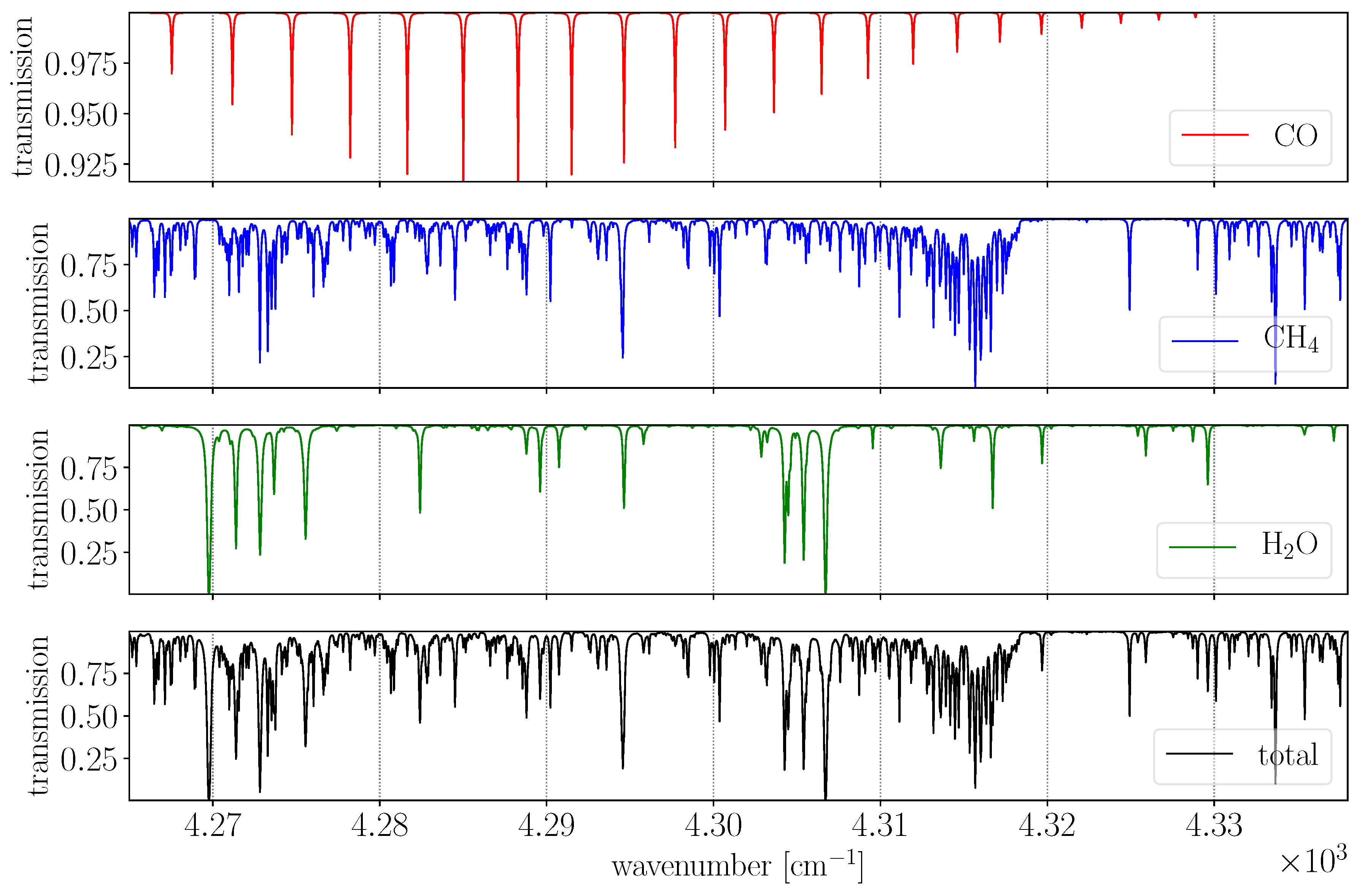
1.3. Absorption in the SWIR and Retrieval

In the SWIR, the fraction of photons generated by thermal emission is well below 1% and can hence be neglected [22]. Furthermore, clear sky measurements are subject to little atmospheric scattering, and most of the measured light is reflected by the Earth’s surface. Those characteristics and TROPOMI’s high signal-to-noise ratio (SNR) in the $2.3\mathsf{\mu }\mathrm{m}$ region over land surfaces allows the instrument to measure clear-sky $\mathrm{CO}$ columns with high sensitivity throughout the vertical extent of the atmosphere [23,24,25,26,27,28,29].

Our retrieval relies on measurements of the first overtone 2-0 absorption band of $\mathrm{CO}$ situated between 3780–4355 ${\mathrm{cm}}^{-1}$ from which the vertically integrated $\mathrm{CO}$ column density is inferred. Since the absorption of $\mathrm{CO}$ is weak in that spectral region (Figure 1), no vertical profile of $\mathrm{CO}$ can be retrieved in the selected fitting window between 4277.20–4302.90 ${\mathrm{cm}}^{-1}$. Furthermore, the least squares fit of the forward model parameters to the measurement depends on initial guess data in order to get an appropriate linearization point for the unconstrained fit.

In order to infer the amount of atmospheric constituents from an observed spectrum, an accurate description of molecular absorption at different pressure p and temperature T levels is mandatory. In high resolution line–by–line (lbl) models, the cross section of a molecule $k_m$ is calculated by the superposition of many lines l, where each line is the product of a temperature dependent line strength $S_l^{\left(m\right)}$ and a normalized line shape function $\underset{-\infty }{\overset{+\infty }{\int }}g\left(\nu \right)\mathrm{d}\nu =1$ that is describing mechanisms, such as pressure and Doppler broadening [31]. Therefore, the best possible knowledge of the spectral parameters, such as line position $\widehat{\nu }$, line intensity S, line width $\gamma$ (air- and self-broadening), temperature exponent n, lower-state energy E, and their variation with T and p, is required. However, advances in high resolution absorption spectroscopy and the advent of sensors, such as TROPOMI, with wide spectral ranges at rather high spectral resolutions and excellent SNR ratios have indicated discrepancies between spectroscopic models and observations [32,33,34,35,36,37]. It was found that physical processes beyond broadening mechanisms described by the Voigt function should be taken into account for accurate atmospheric characterization. Moreover, studies [24,38,39,40,41,42] also indicate that improved molecular spectroscopy is crucial to eliminate systematic residuals in atmospheric spectra and that trace gas retrievals in the SWIR will benefit accordingly.

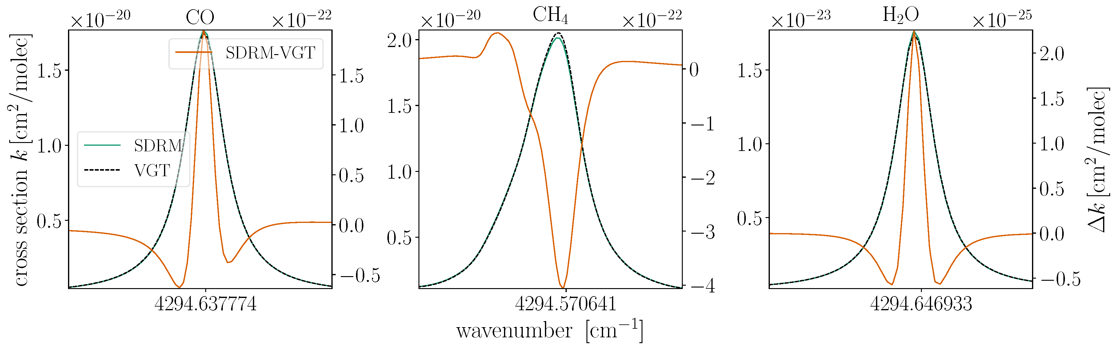
1.4. Spectroscopic Line Data and Line Profiles

The SEOM–IAS (SEOM, Scientific Exploitation of Operational Missions–Improved Atmospheric Spectroscopy) is an improved line parameter database of ${\mathrm{H}}_2\mathrm{O}$, ${\mathrm{CH}}_4$, and $\mathrm{CO}$ (available on Zenodo [43,44]) compiled within the framework of an ESA project according to the needs of the TROPOMI instrument. Fourier transform spectrometer (FTS) and continuous wave cavity ring-down spectroscopy (CRDS) measurements (performed at the German Aerospace Center (DLR) and at Université Grenoble Alpes, respectively) were analyzed in the 4190–4340${\mathrm{cm}}^{-1}$ spectral range. The spectroscopic database was obtained from high resolution FTS measurements employing a multireflection cell with absorption path lengths from 14.4–168 m and a temperature range 198–361 K (12 pure and 32 air-broadened ${\mathrm{CH}}_4$ measurements, 1 pure and 4 air-broadened $\mathrm{CO}$ measurements, 7 pure and 23 air-broadened ${\mathrm{H}}_2\mathrm{O}$ measurements, and 4 pure $\mathrm{HDO}$ measurements). A multispectrum fitting software [45] developed at DLR was used for the analysis of the measured spectra. For modeling of absorption lines in the multispectrum fitting, a quadratic speed-dependent hard collision model based on the implementation of the Hartmann-Tran (HT) profile was used [35,46,47,48,49]. In order to account for line-mixing, the profile was extended using the first and second order perturbation approximation by Rosenkranz [50] and Smith [51]. The CRDS measurements served as validation.

The HT profile with vanishing correlation ($\eta =0$) reduces to the speed-dependent Rautian (SDR [52,53,54,55,56,57]) profile. The transmissions in Figure 1 were computed with line-mixing included, i.e., the SEOM with Speed-Dependent Rautian and line-Mixing (SDRM) profile. Figure 2 shows a close up view of the molecular cross sections for $\mathrm{CO}$, ${\mathrm{CH}}_4$, and ${\mathrm{H}}_2\mathrm{O}$ near $4295{\mathrm{cm}}^{-1}$, where all three molecules possess a fairly strong and almost co-located transition. For each molecule, two cross sections were calculated, one with the SDRM profile (including the extended set of line data) and another with the classic Voigt model, while both use SEOM line data as input. The differences between the two turned out to be around two orders of magnitude smaller than the actual cross sections itself with the maximum disagreement located close to the line center positions.

1.5. Previous Studies

An initial validation of SEOM tested the line list with atmospheric spectra from solar occultation measurements, and the new database was found to be a significant improvement over High Resolution Transmission (HITRAN) 2016 (M. Birk, personal communication).

An assessment of the operational TROPOMI $\mathrm{CO}$ product for various spectroscopic inputs, including SEOM, was recently published by Borsdorff et al. [58]; however, only the spectroscopic data was substituted, while the remaining retrieval settings were identical to the ones of the operational processing. The study quantified the quality of the spectral fits and biases in the $\mathrm{CO}$ column and found that “updating the ${\mathrm{CH}}_4$ cross sections is the main reason for the improved $\mathrm{CO}$ product”. They concluded that molecular spectroscopy data plays a key role for the quality of the retrieval.

In a recent study [59], we examined the impact of SEOM spectroscopic information on $\mathrm{CO}$ total columns from SCIAMACHY and found that the best retrieval results for SEOM line data are obtained when higher-order ‘beyond Voigt’ effects in molecular absorption are taken into account. The outcome indicates that, strictly speaking, the classic Voigt profile is not an adequate line model for the SEOM line list (confirmed by M. Birk, personal communication), although the largest impact on the improved fitting residuals ($\approx 3\%$ on average, up to 15% for individual observations) is attributed to the updated line parameters while the line profile has less contribution. Although the $\mathrm{CO}$ mole fractions increased by $4-11\%$ using SEOM spectroscopy the difference to H16 was found to be significant for only a limited set of spectra (see Reference [59, Figure 7 and A4]).

2. Methodology

In this study, we investigated the impact of the SEOM spectroscopy on the retrieved $\mathrm{CO}$ from TROPOMI SWIR observations by comparing the spectral fitting residuals, deduced columns, and corresponding retrieval errors with the most recent releases of HITRAN 2016 (H16, High Resolution Transmission; [60]) and GEISA 2015 (G15, Gestion et Etude des Informations Spectroscopiques Atmosphériques 2015 [61]). Besides the target gas $\mathrm{CO}$, the impact on the interfering, and hence co-retrieved species ${\mathrm{CH}}_4$ and ${\mathrm{H}}_2\mathrm{O}$ (including their isotopologues), was examined. Note that the reason to stay with the current version of GEISA (2015 instead of 2019) was that not all molecules required for the retrieval of $\mathrm{CO}$ in the specified spectral range were updated at the time of submission (R. Armante, personal communication).

2.1. Retrieval Setup

The retrievals in this study were performed with the latest version of the scientific retrieval algorithm BIRRA (Beer Infrared Retrieval Algorithm [25,62]) which has been developed at the German Aerospace Center (DLR) since about 2005. In addition to enhancements in the GARLIC (Generic Atmospheric Radiation Line-by-line Infrared Code [63,64]) forward model described in [59], this most recent version of BIRRA incorporates TROPOMI calibration key data (CKD), such as tabulated instrument spectral response functions (ISRF).

2.2. Input Data

An updated framework is providing auxiliary data for the prototype retrieval of $\mathrm{CO}$ abundances from TROPOMI. Since information on the amount of $\mathrm{CO}$ is inferred by optimally varying forward model parameters during the inversion process, the quality of the input data affects the accuracy of the retrieval.

2.2.1. Calibrated Level 1b Spectra

The TROPOMI level 1b data (version 1.0) from band 7 contains spectrally and radiometrically calibrated Earth radiance and solar irradiance spectra in the 2305–2345$\mathrm{nm}$ (≈ 4338–4265 ${\mathrm{cm}}^{-1}$) spectral range (see Figure 3). These quantities already include corrections from the CKD that account for several effects, such as offset, dark-current, pixel-quality, non-linear response, and noise, and were derived during the on-ground calibration campaign prior to launch [65,66]. In-flight, the CKD of, e.g., the pixel-quality, the ISRF, and stray-light correction, is monitored by TROPOMI’s calibration unit and updated over the lifetime of the instrument if necessary. This is crucial as the operational level 0-1b processor marks data with quality assessment flags, e.g., in order to exclude bad and dead pixels that are deemed unusable for generation of the level 2 product. The actual number of available pixels in the selected retrieval window between 4277.20–4302.90 ${\mathrm{cm}}^{-1}$ is dependent on the bad and dead pixel-mask (BDPM) and ranges from 146–154 for observations considered in this study. Note that TROPOMI is commanded to perform a solar irradiance measurement near the day-night terminator at the northern side of the orbit only every 15 orbits, i.e., approximately once every calendar day [10].

2.2.2. The Instrument’s Spectral Response

The forward model needs to include an accurate description of the ISRF $\mathcal{S}$ in order to model the physics of the measurement with adequate accuracy. In the SWIR, the TROPOMI ISRFs vary across the spectral and spatial dimension ${\mathcal{S}}_{ij}$ and are provided for each of the $1\le i\le 256$ ground pixels, as well as for $1\le j\le 24$ equally spaced central wavelengths of the spectral axis ranging from 2298 to 2344 nm [68]. Eight tabulated ISRFs remain within the range of sufficiently strong $\mathrm{CO}$ absorption lines defining our fitting window; hence, interpolated response values were used for most spectral pixels. The rather smooth variation in the spectral dimension is beneficial for the interpolation of responses to pixels where no tabulated values are available (see Figure 4 and Figure 5). Nonetheless, accounting for those variations in the instrument’s response is important, particularly when testing spectroscopic data and models.

During on-ground calibration, van Hees et al. [68] found that the accuracy of the ISRF CKD is well within the requirements for trace-gas retrievals. Moreover, van Kempen et al. [66] found that the differences between in-flight and on-ground CKD measurements are small, and no corrections need to be applied.

2.2.3. Atmospheric Input Data

The physical description of a measurement by the forward model requires input for some atmospheric state-variables, such as pressure p, temperature T, and specific humidity q, since, e.g., the cross section of molecules $k_m$ need to be calculated at different atmospheric levels in order to accurately model lbl absorption through the atmosphere.

Note that BIRRA [25] in Section 2.2.2 utilizes a separable least squares where the state-vector $\mathbf{x}$ is separated into two vectors $\mathit{\eta }\subset \mathbf{x}$ and $\mathit{\beta }\subset \mathbf{x}$ comprising the linear and nonlinear parameters [70], and that initial guess values are only required for the nonlinear parameters. In the forward model, the ‘true’ optical depth of a molecule ${\tau }_m$ is described as

$${\tau }_m\left(\nu \right)={\alpha }_m{\tau }_m^{\mathrm{ref}}\left(\nu \right)={\alpha }_m\underset{\begin{array}{c}\mathrm{double}\\ \mathrm{path}\end{array}}{\int }{n}_m^{\mathrm{ref}}\left(s\right)k_m(\nu ,s)\mathrm{d}s,$$

(1)

with ${\alpha }_m\in \mathit{\eta }$ and $n_m^{\mathrm{ref}}$ the initial guess molecular number density. In Figure 6, the initial guess for $\mathrm{CO}$ and ${\mathrm{CH}}_4$ mole fractions are shown. Both resemble AIRS (Atmospheric Infrared Sounder) version 6 initial guess profiles [71,72] with varying concentrations from the northern hemisphere to the southern hemisphere. The AIRS $\mathrm{CO}$ initial guess comes from MOZART (Model for OZone And Related chemical Tracers [73]) monthly mean hemispheric profiles, while ${\mathrm{CH}}_4$ is described by a function of latitude and altitude. Pressure and temperature, as well as the specific humidity, were taken from the 4-times daily reanalysis product [74] maintained by the National Center for Environmental Prediction (NCEP).

2.2.4. Cloud Filtering and Topographic Information

Auxiliary input data on clouds was obtained from the S5P-NPPC product which is available for the TROPOMI bands 3, 6, and 7 (SWIR). The Visible Infrared Imaging Radiometer Suite (VIIRS [75]) aboard the Suomi-NPP (Suomi National Polar-Orbiting Partnership [76,77]) spacecraft leads ahead the S5P in loose formation orbit by 3.5 min in local time ascending node and reports cloud information with high spatial resolution on nominal and scaled TROPOMI field of views (FOV). The cloud mask data is grouped in four classes, namely confidently cloudy, probably cloudy, probably clear, and confidently clear. Prior to the $\mathrm{CO}$ retrieval the cloud fraction was calculated for the 1.5 scaled FOV of TROPOMI’s band 7 (in the along and across-track dimension), and the ratio of the ‘confident’ and ‘probable’ classifications was formed. Besides the retrieved ${\mathrm{CH}}_4$ absorption, those quantities serve to identify conditions that might lead to errors in the retrieved columns due to path modifications by clouds and aerosols (scattering) of the observed light, which is not yet considered in the forward model. In particular, an observation was rejected if the cloud fraction specified in the S5P-NPPC product exceeds 10% or if the number of VIIRS pixels that fall into the ‘probable’ classification (i.e., not the ‘confident’ classification) exceeds 20%. These rigorous filter criteria avoid observations with large retrieval inaccuracies caused by scattered photons [78] and minimize any bias that arises from changes in the retrieval’s vertical sensitivity by modifications in the column averaging kernel (CAK [23], Section 5) in Figure 7 (also see Reference [28], Section 3, and Figure 4 [79] and Figure 3).

Furthermore, the calculation of the double-path transmission between the reflection point (e.g., Earth’s surface) and observer and between Sun and reflection point (see Equation (1)) requires topographic information on terrain elevation. Therefore, the ETOPO global relief model [80] with 2-min grid spacing and an adequate vertical and horizontal datum provides elevation data for each TROPOMI observation in the radiative transfer calculation.

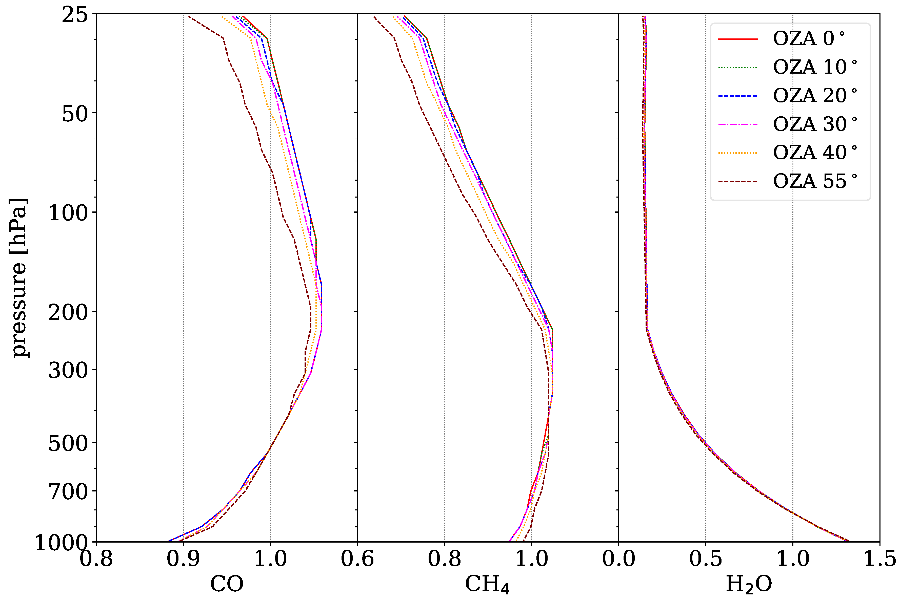
2.3. Vertical Sensitivity and Relation to Priors

In the context of profile retrievals, the sensitivity of the inversion process to the true atmospheric state is given by the averaging kernel. Nonetheless, column density retrievals also have some altitude dependent sensitivity, i.e., the perturbation of elements in the state-vector $\mathbf{x}$ at different altitudes result in a non-uniform retrieval response [81] (Section 2 and Section 3).

Figure 7 shows the altitude sensitivity for three elements of BIRRA’s state-vector. The vertical sensitivity for the target gas and ${\mathrm{CH}}_4$ reveals to be close to unity across the full range of TROPOMI observer zenith angles (OZA), while the CAK of ${\mathrm{H}}_2\mathrm{O}$ tends towards zero at higher altitudes, where the retrieval is less sensitive to the true atmospheric state.

2.4. Assessing the Quality of the Fit

Standard diagnostics are used to assess deficiencies in the forward model of the retrieval. In particular, the scaled 2-norm of the spectral fitting residual

$$\rho ={\mathbf{I}}_{\mathrm{obs}}-\mathbf{I}\left(\mathbf{x}\right),$$

(2)

$${\sigma }^2={\left|\right|\rho \left|\right|}^2/(m-n)$$

(3)

is a suitable criterion as it becomes smaller the better the forward model $\mathbf{I}\left(\mathbf{x}\right)$ can mimic the measurements ${\mathbf{I}}_{\mathrm{obs}}$. Note that m is designating the number of available TROPOMI measurements in our fitting window and is dependent on the BDPM (see Section 3). n is the number of elements in the state-vector $\mathbf{x}$ which is constant and in the setup for this study includes the molecular scaling factors $\mathit{\alpha }\subseteq \mathit{\eta }$ and a second-degree polynomial in wavenumber $\mathbf{r}\subseteq \mathit{\beta }$ representing the surface reflectivity.

Furthermore, it is important to note that the absolute value of ${\sigma }^2$ is dependent on the SNR and since no normalization is applied, strictly speaking, only residuals from the same observation should be compared against each other. Nonetheless, it is deemed permissible to compare the scaled norm of the fitting residual within a region as the environment is quite homogeneous in terms of temperature, humidity, and, even at TROPOMI’s spatial resolution, surface reflectance.

Errors in molecular spectroscopy can introduce systematic spectral residuals that in consequence result in larger retrieval errors of the corresponding quantities according to

$$\mathsf{\Xi }={\sigma }^2{\left(J^{\mathrm{T}}J\right)}^{-1}.$$

(4)

The least squares covariance matrix $\mathsf{\Xi }$ contains the Jacobians $J\equiv \frac{\partial \mathbf{I}}{\partial \mathbf{x}}$ of the fitted parameters and diagonal elements represent the errors of the state-vector components [25,82]. Therefore, besides the analysis of the residual norms in Section 3.1, the fitted state-vector elements $\mathit{\alpha }$, along with their error estimates, are examined in Section 3.2.

3. Results

The investigation was performed for a set of TROPOMI orbits in 2019 that cover various climatological regions, namely the Sahara, Central-Europe, Amazonia, and Siberia (for details, see

Table 1. Average of the scaled norm of the fitting residuals E(${\sigma }^2$) for individual TROPOMI overpasses in 2019.

Input		E(${\mathit{\sigma }}^2$)
Region	Data	Spring	Summer	Fall	Winter	Total
Orbit		6967	7861	8812	10,542
Sahara	G15	$1.93·{10}^{-5}$	$2.69·{10}^{-5}$	$2.40·{10}^{-5}$	$8.65·{10}^{-6}$	$1.97·{10}^{-5}$
	H16	$1.79·{10}^{-5}$	$2.52·{10}^{-5}$	$2.20·{10}^{-5}$	$7.63·{10}^{-6}$	$1.82·{10}^{-5}$
	SDRM	$1.65·{10}^{-5}$	$2.18·{10}^{-5}$	$1.74·{10}^{-5}$	$6.24·{10}^{-6}$	$1.55·{10}^{-5}$
Orbit		6967	7861	8811	10,542
Central-Europe	G15	$5.93·{10}^{-7}$	$8.28·{10}^{-7}$	$7.56·{10}^{-7}$	$6.89·{10}^{-7}$	$7.17·{10}^{-7}$
	H16	$5.95·{10}^{-7}$	$7.70·{10}^{-7}$	$5.72·{10}^{-7}$	$5.92·{10}^{-7}$	$6.32·{10}^{-7}$
	SDRM	$4.92·{10}^{-7}$	$7.11·{10}^{-7}$	$5.70·{10}^{-7}$	$5.65·{10}^{-7}$	$5.84·{10}^{-7}$
Orbit		7581	8517	9553	10,347
Amazonia	G15	$2.29·{10}^{-6}$	$1.16·{10}^{-6}$	$2.93·{10}^{-6}$	$2.80·{10}^{-6}$	$2.30·{10}^{-6}$
	H16	$2.14·{10}^{-6}$	$9.04·{10}^{-7}$	$2.74·{10}^{-6}$	$2.57·{10}^{-6}$	$2.09·{10}^{-6}$
	SDRM	$1.88·{10}^{-6}$	$9.00·{10}^{-7}$	$2.36·{10}^{-6}$	$2.29·{10}^{-6}$	$1.86·{10}^{-6}$
Orbit		7348	8231	9093	9958
Siberia	G15	$1.45·{10}^{-6}$	$2.11·{10}^{-6}$	$2.94·{10}^{-6}$	$1.25·{10}^{-6}$	$1.94·{10}^{-6}$
	H16	$1.33·{10}^{-6}$	$1.93·{10}^{-6}$	$2.81·{10}^{-6}$	$1.15·{10}^{-6}$	$1.81·{10}^{-6}$
	SDRM	$1.29·{10}^{-6}$	$1.14·{10}^{-6}$	$2.62·{10}^{-6}$	$1.14·{10}^{-6}$	$1.55·{10}^{-6}$

). Aside from Central-Europe, the areas were selected according to different pairs of temperature and humidity values, and Europe contains strong anthropogenic sources (cities, large harbors, airports, etc.), as well as $\mathrm{CO}$ background levels (rural areas, many alpine regions, etc.). The individual orbits are given in Table 1 and were selected based on (low) cloud coverage. Nonetheless, post-processing steps include rigorous cloud filtering, the removal of non-converged retrievals, and the disposal of measurements with very small SNRs (e.g., observations above large bodies of water, such as lakes, rivers, etc.).

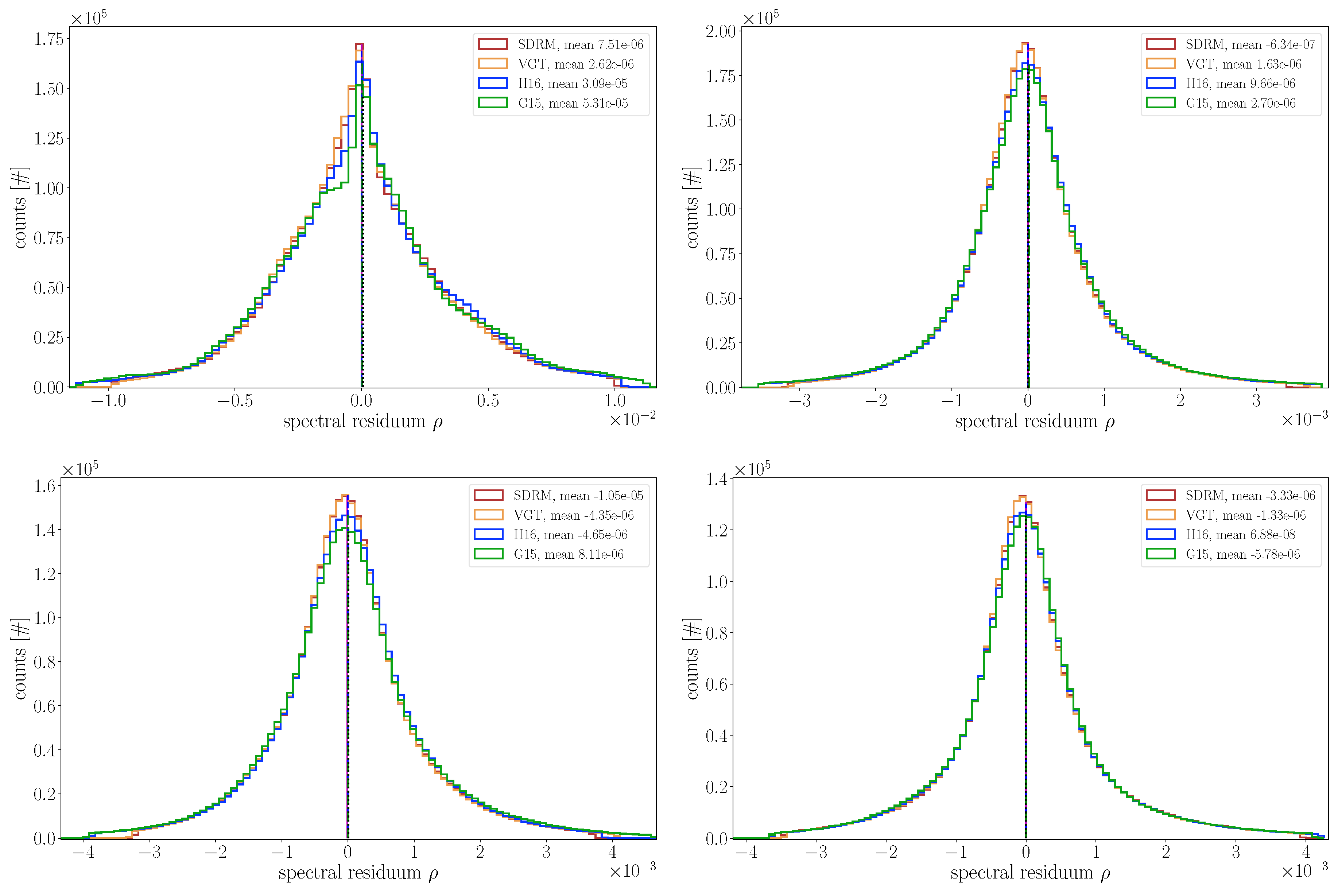
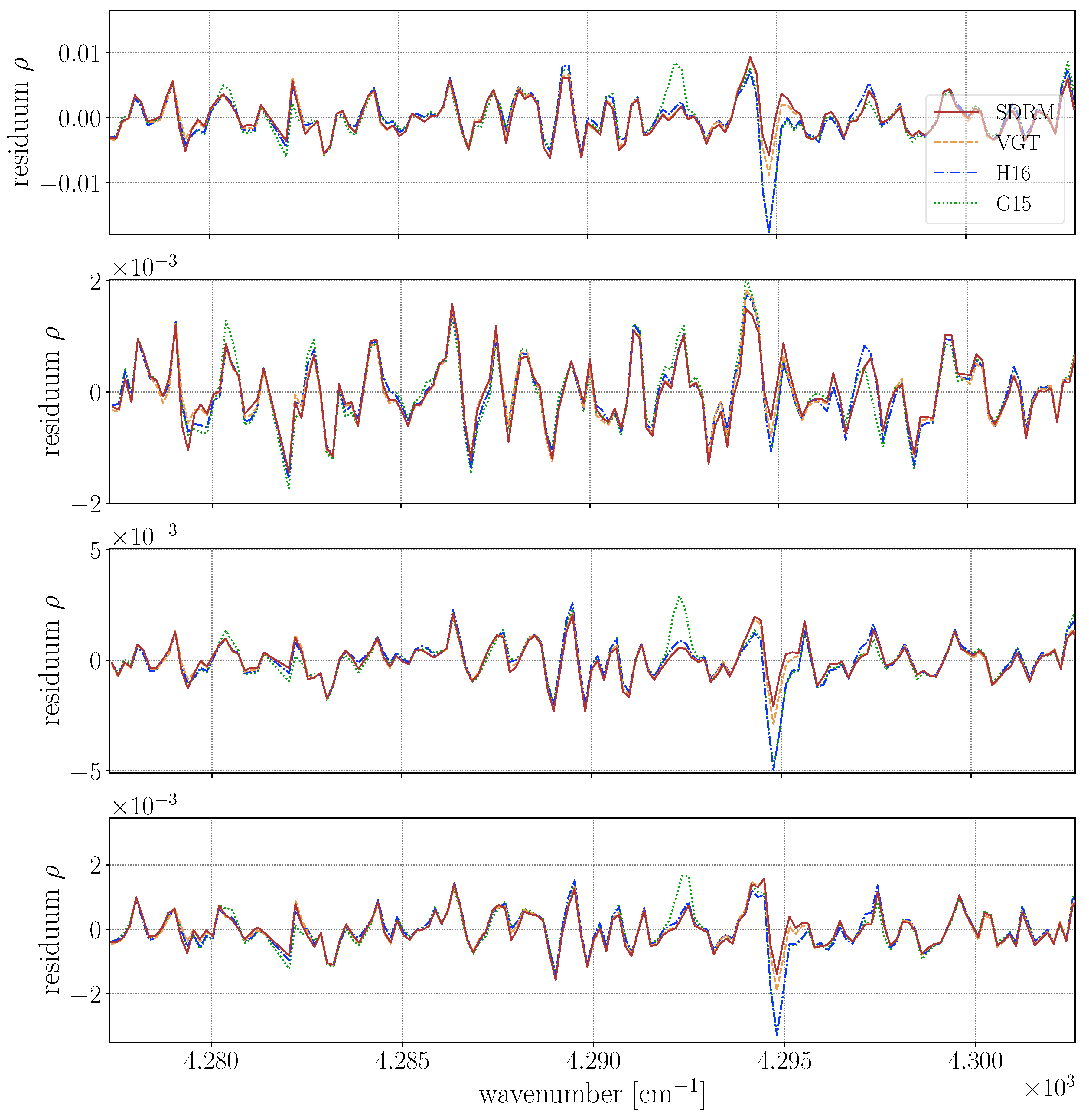
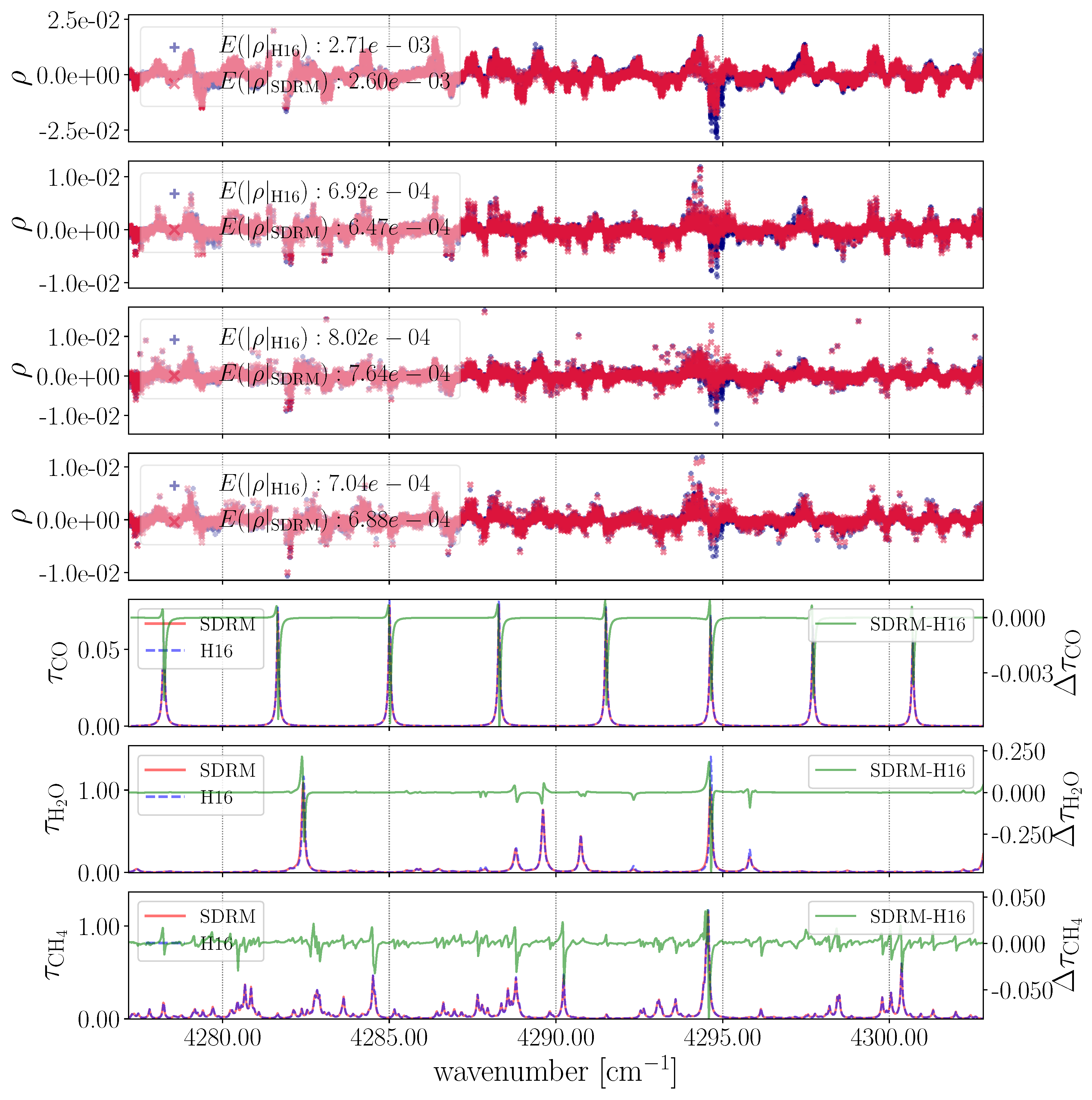
3.1. Spectral Fitting Residuals

The elements of the residual vectors according to Equation (2) are depicted in Figure 8. The histograms are separated by regions, starting with Sahara at the top-left and depicting Central-Europe, Siberia, and Amazonia in the clockwise direction. The residuals are following a normal distribution (except for Sahara) with an expected value around zero, indicating that the majority of the measurement errors are caused by random errors, such as instrument noise, etc. This is crucial in order to get the so-called best linear unbiased estimate for the state-vector $\mathbf{x}$ [83]. In the Sahara region, however, the distribution of residuals deviate from the Gaussian form in particular around the center of the curve and most significantly for G15. The non-uniform distribution over the Sahara is reduced for the SDRM retrievals. Note that the SEOM-Voigt case only considers spectral parameters that describe the mechanisms of pressure and Doppler broadening and was included in order to discriminate the impact of line data versus model.

Figure 9 shows one residual vector for a randomly picked measurement per region. It reveals that the modeled spectra for both H16 and G15 exhibit the largest disagreements in a spectral region close to $4295{\mathrm{cm}}^{-1}$. This feature is significantly reduced when using SEOM line data and virtually eliminated when the SDRM line profile is applied (see Figure 2), as well causing a rather uniform distribution of the residuals across wavenumbers. In addition, G15 reveals some discrepancy round $4293{\mathrm{cm}}^{-1}$. Note that spectral ranges with increased differences show the same positive or negative deviations across geographic regions, indicating that the radiance (transmission) is persistently over- or underestimated for those wavenumbers.

In Figure 10, the individual detector-pixel residuals are examined for all measurements across seasons. The average of the absolute differences is given by $E\left(\right|\rho \left|\right)$. It shows that the pixels close to $4295{\mathrm{cm}}^{-1}$ consistently exhibit major disagreements and that the retrievals over the Sahara (first panel) show the largest discrepancies on average since the absolute values of the elements in $\rho$ are dependent on the SNR (see Section 2.4). Furthermore, in order to identify molecular transitions that possibly cause the discrepancies, optical depths of the absorbing molecules $\mathrm{CO}$, ${\mathrm{CH}}_4$, and ${\mathrm{H}}_2\mathrm{O}$ are depicted in three separate but aligned panels below. It becomes obvious that the disagreements around $4295{\mathrm{cm}}^{-1}$ coincide with three rather strong and overlapping absorption lines that were shown in Figure 2. SDRM and H16, particularly, do not agree in that part of the spectrum, and the overall spectral fit quality is improved by $\approx 4-8\%$ for SDRM retrievals.

The substitution of H16 line data with SDRM for each molecule individually shows that the impact on the fit quality is small when $\mathrm{CO}$ is replaced (<0.5%) but improves considerably when ${\mathrm{H}}_2\mathrm{O}$ (>7%) and ${\mathrm{CH}}_4$ (>5%) is updated. The given numbers are averages across all investigated regions. Since the residuals for G15 are similar with respect to H16 (except for some pixels between 4280–4285${\mathrm{cm}}^{-1}$ and around $4293{\mathrm{cm}}^{-1}$ as indicated in Figure 9), they are not depicted in Figure 10.

The averages of the scaled norm ${\sigma }^2$ are itemized by region and season in Table 1. The results confirm above-mentioned findings, i.e., the retrievals using SEOM line data effectively cause smaller discrepancies to TROPOMI observations. More precisely, SDRM-based retrievals reduce ${\sigma }^2$ with respect to H16 and G15 by approximately 10–15$\%$ and 15–20$\%$, respectively. The smaller disagreements between SDRM and H16 are likely attributed to the fact that both are not completely independent sets of line data and some of the updates from SEOM are already included in H16 [58].

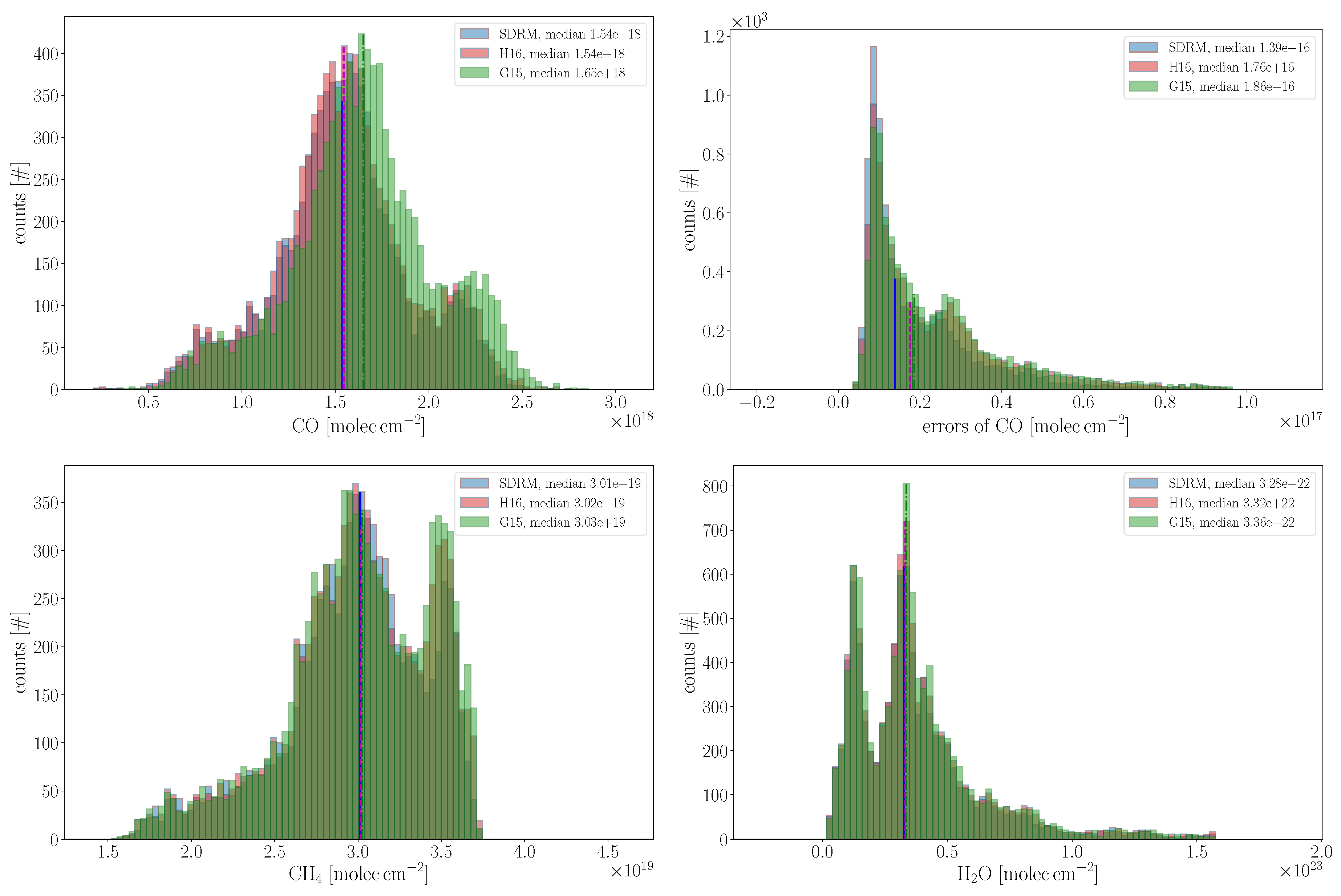
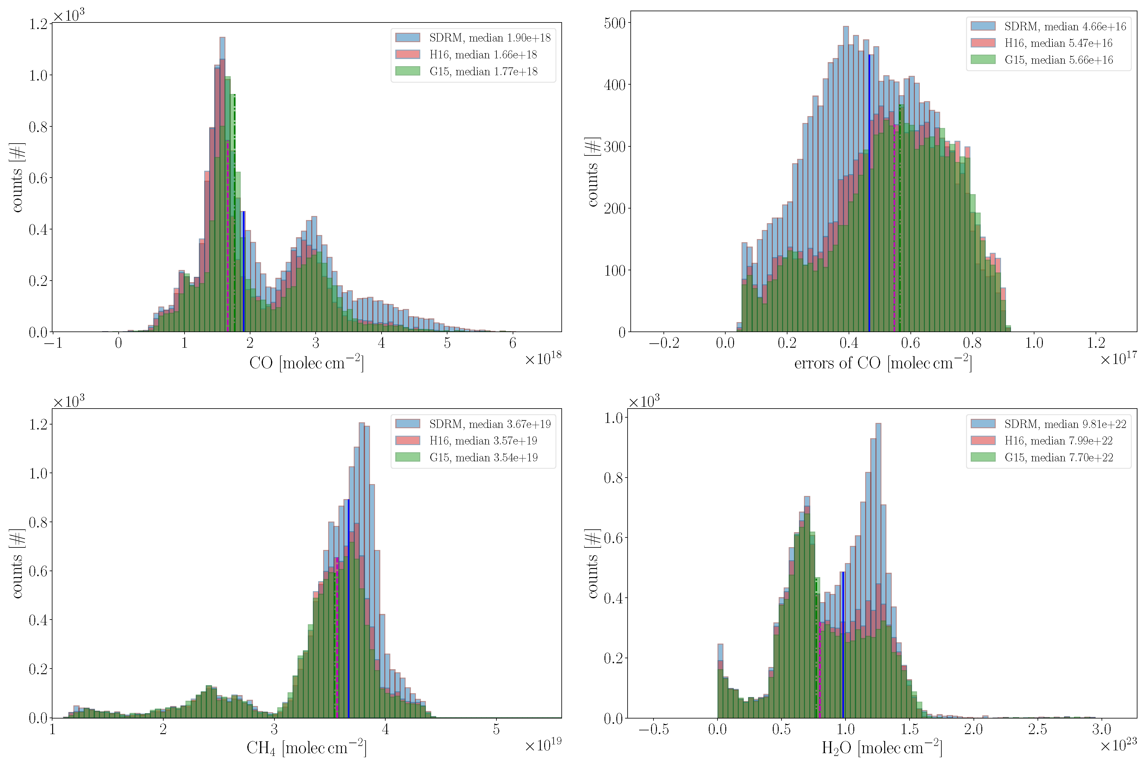
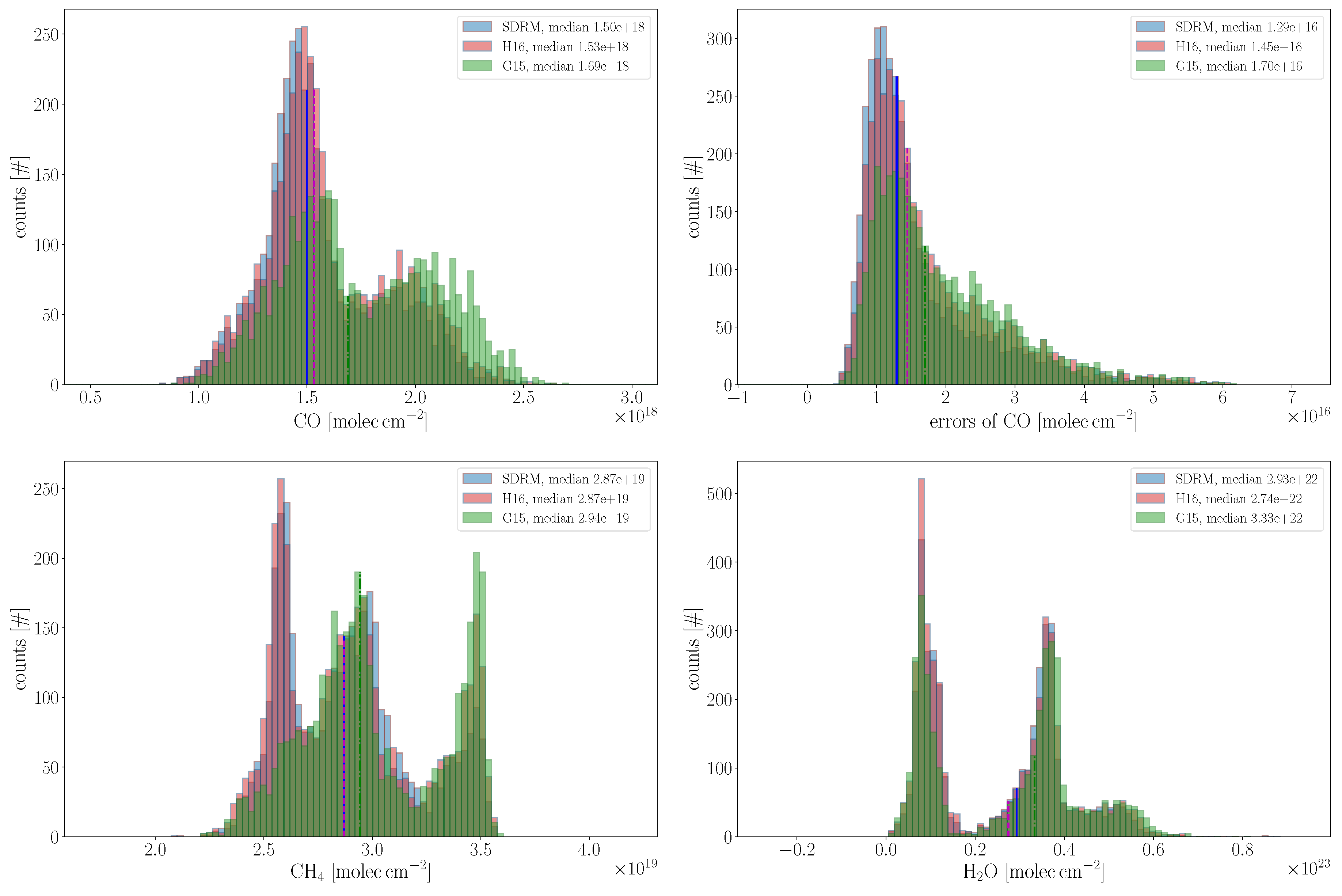
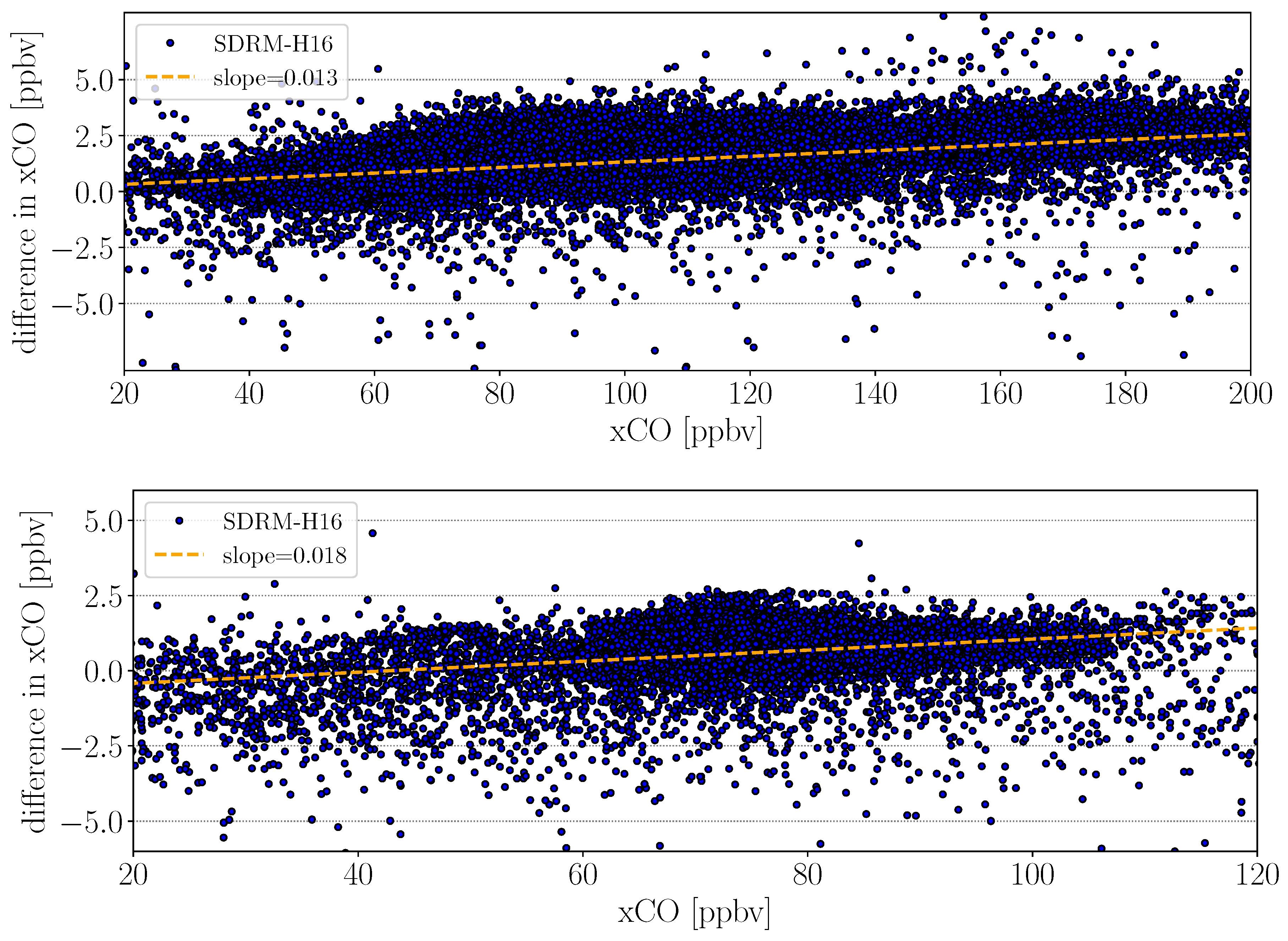
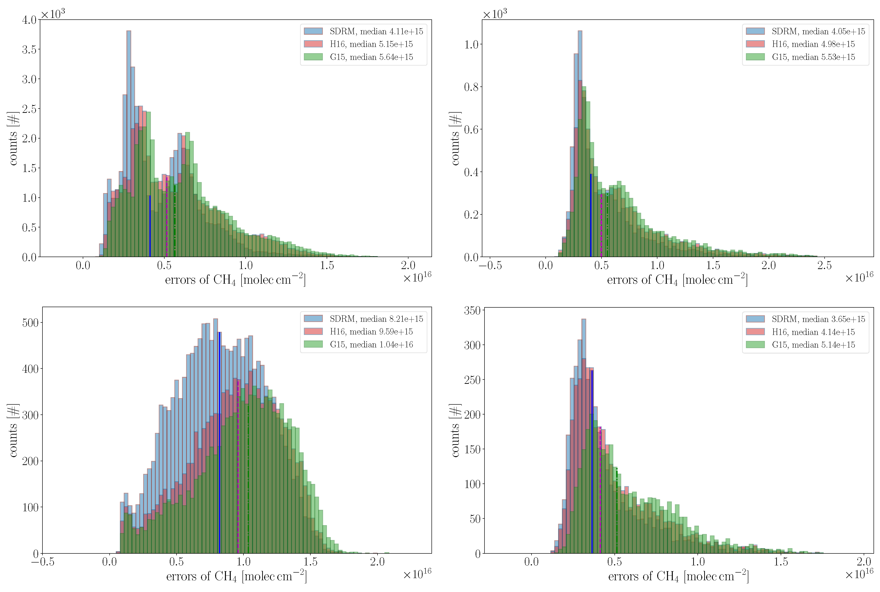
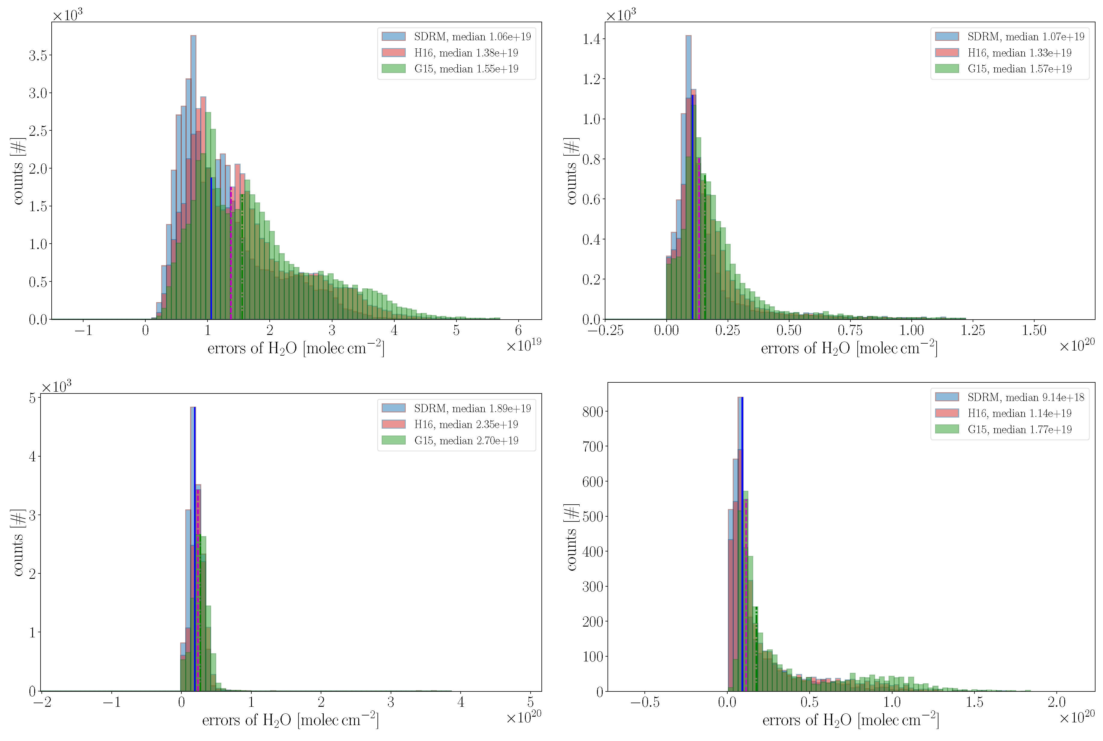
3.2. Impact on Retrieved Columns and Corresponding Errors

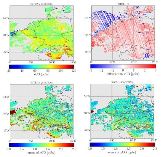
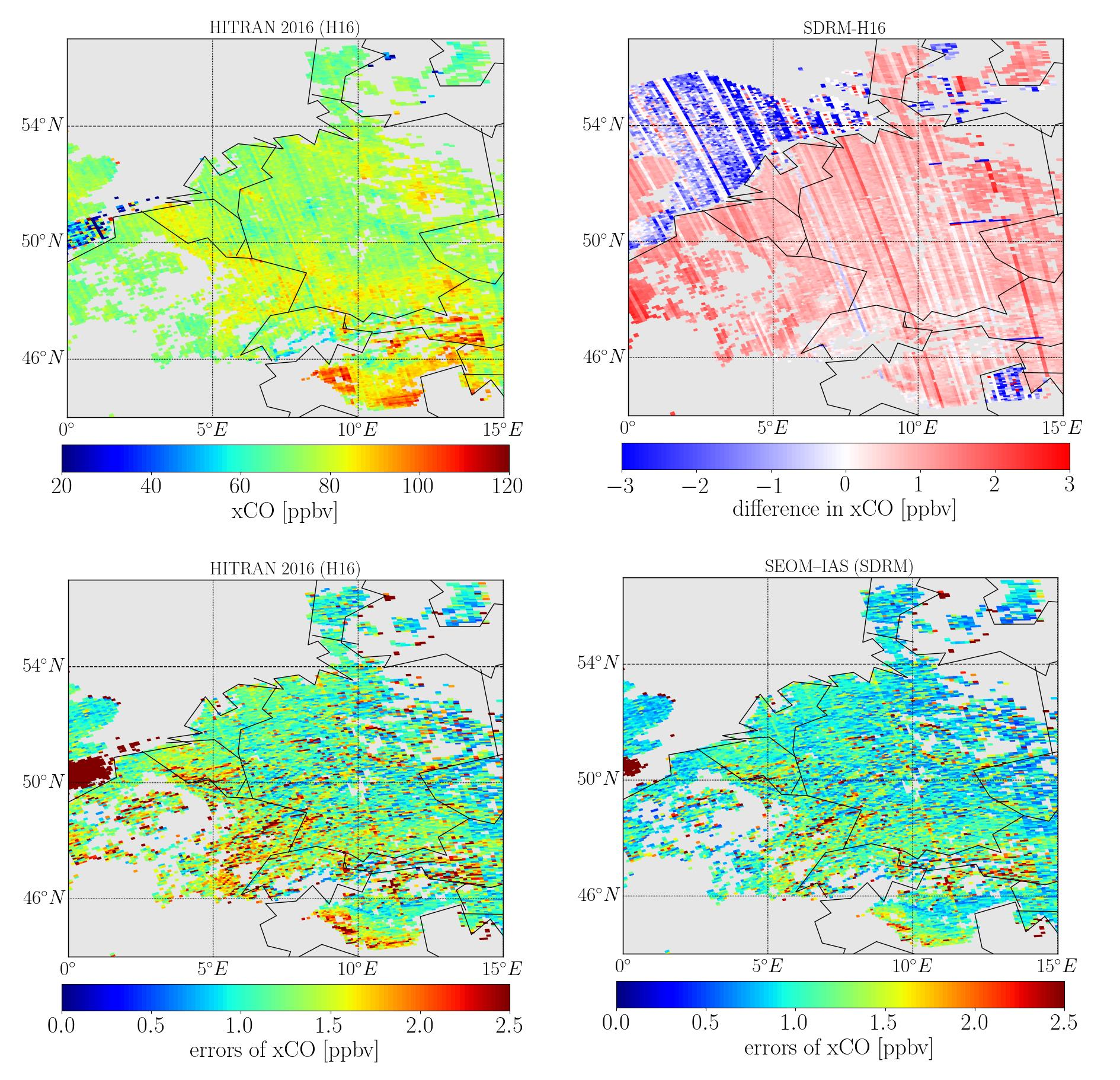
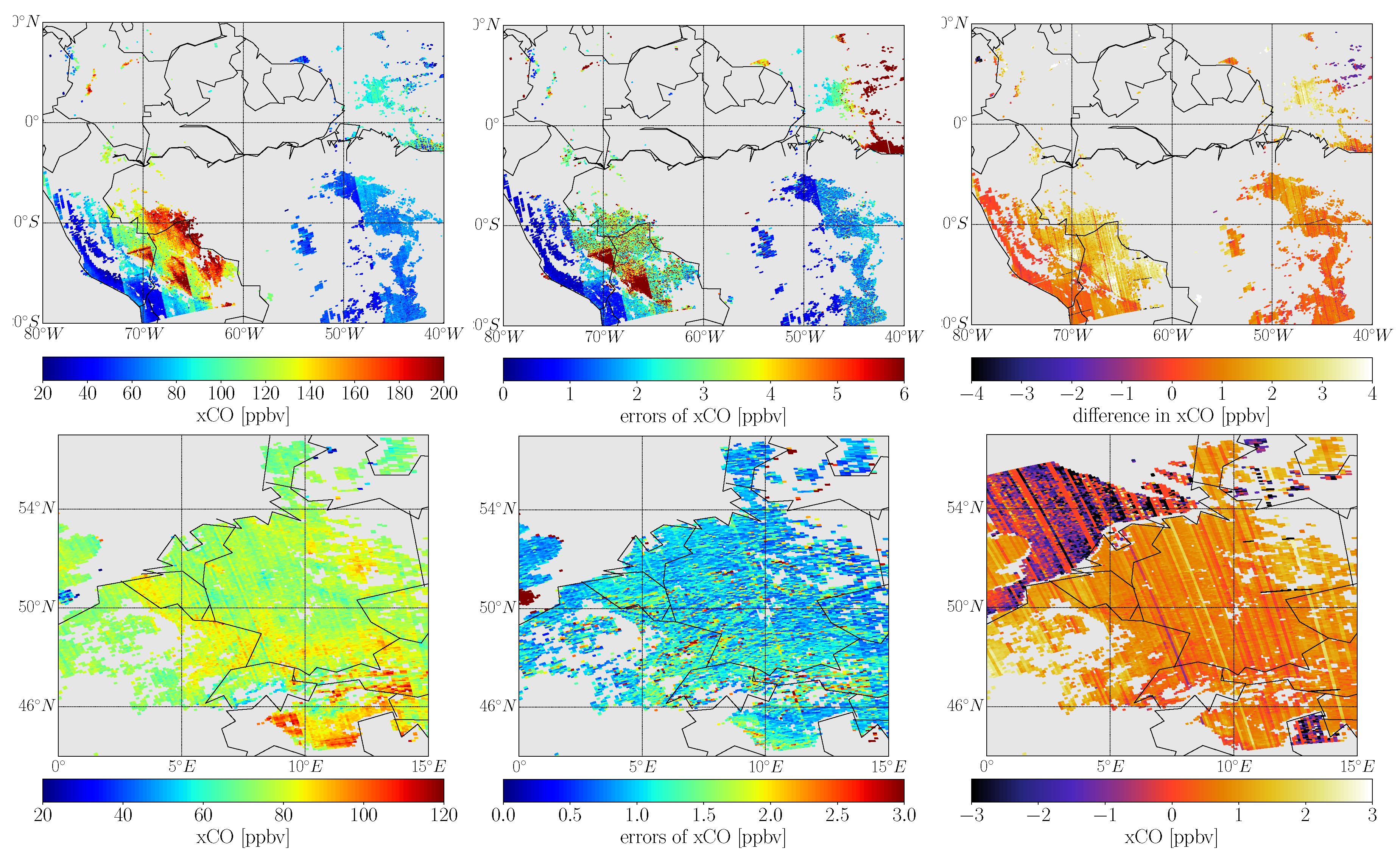
The effect of absorption line data on the retrieved $\mathrm{CO}$ total columns $N_m\left[\mathrm{molec}{\mathrm{cm}}^{-2}\right]$ and corresponding errors is shown in Figure 11, Figure 12, Figure 13 and Figure 14. Each figure depicts the results for one region and contains the target and co-retrieved quantities according to

$$N_m={\alpha }_m\underset{{\mathrm{z}}_{\mathrm{srf}}}{\overset{{\mathrm{z}}_{\mathrm{TOA}}}{\int }}{n}_m^{\mathrm{ref}}\left(z\right)={\alpha }_m{N}_m^{\mathrm{ref}}.$$

(5)

The mole fractions for some molecular number densities $n_m^{\mathrm{ref}}$ are shown in Figure 6. It is important to note that ${\mathrm{H}}_2\mathrm{O}$ and ${\mathrm{CH}}_4$, although the latter has strong absorption lines across the $\mathrm{CO}$ spectral fitting window and can be used to identify light path modifications [78], are byproducts primarily considered due to their spectral interference with the target gas. The distribution of the errors for ${\mathrm{CH}}_4$ and ${\mathrm{H}}_2\mathrm{O}$ is shown in Appendix A.

For the Sahara region depicted in Figure 11, the majority of $\mathrm{CO}$ is distributed between $1.0-2.5·{10}^{18}\mathrm{molec}{\mathrm{cm}}^{-2}$ and the histograms for SDRM and HITRAN are similar. The $\mathrm{CO}$ retrieval errors according to Equation (4) are illustrated in the top-right and are below $1.0·{10}^{17}\mathrm{molec}{\mathrm{cm}}^{-2}$ across spectroscopies with the median around $1.7·{10}^{16}\mathrm{molec}{\mathrm{cm}}^{-2}$ in case of SDRM and around $2.2·{10}^{16}\mathrm{molec}{\mathrm{cm}}^{-2}$ for the other two line lists. Note that the majority of the $\mathrm{CO}$ errors for SDRM are even below $6.0·{10}^{16}\mathrm{molec}{\mathrm{cm}}^{-2}$. Although there is almost no absolute difference in the medians of the $\mathrm{CO}$ columns for SDRM and H16 distributions, they were found to be significantly different according to the non-parametric Kolmogorov-Smirnoff test (p-value $<1.0·{10}^{-5}$) [84]. While this holds true for SDRM and G15 distributions ($\mathrm{CO}$ difference ≈ $1.0·{10}^{17}\mathrm{molec}{\mathrm{cm}}^{-2}$), the magnitude of their retrieval errors is significantly different, as well.

A similar $\mathrm{CO}$ distribution is observed for Central-Europe in Figure 12, but values cover a greater range. Again, SDRM and H16 cause similar concentrations, while G15 is significantly different based on the distribution of errors. Moreover, the SDRM-based $\mathrm{CO}$ product is, again, the most precise, i.e., incorporates the smallest fitting residuals and thus retrieval errors.

In Figure 13, the $\mathrm{CO}$ columns over Amazonia show a rather different distribution where SDRM retrievals cause significantly higher concentrations. The difference is also significant for the two co-retrieved molecules. The errors in the top-left are larger compared to the two previous regions; however, SDRM-based errors are, again, the smallest. The difference in $\mathrm{CO}$ for both SDRM-H16 and SDRM-G15 was found to be $2.4·{10}^{17}$ and $1.3·{10}^{17}\mathrm{molec}{\mathrm{cm}}^{-2}$, respectively. The errors are consistently <$1.0·{10}^{17}\mathrm{molec}{\mathrm{cm}}^{-2}$ which indicates that the differences in SDRM retrieved $\mathrm{CO}$ concentrations over Amazonia are significant with respect to both other line lists, suggesting that the ‘true’ value might be outside the specified error range of the product. Furthermore, it should be noted that the S5P-overpass in the second quarter.

The distribution of $\mathrm{CO}$ over Siberia in Figure 14 is similar to that for Sahara and Central-Europe, i.e., the histograms for SDRM and HITRAN almost resemble each other, while GEISA is shifted towards higher columns on average. Again, this shift is larger than the product error and thus considered to be significant. In contrast to the other regions, the ${\mathrm{CH}}_4$ columns for G15 are also shifted. For ${\mathrm{H}}_2\mathrm{O}$, the medians are rather equally spaced across cases as it is true for the errors.

3.3. $\mathrm{CO}$ over Amazonia and Central-Europe

The trend of differences between SDRM and H16-based $\mathrm{CO}$ mole fractions over Amazonia and Europe is depicted in Figure 15. The standard set of filter criteria described in Section 3 was applied on a mostly sunny, high pressure influenced day over Central-Europe on 21 September 2019 (orbit 10046) and a day with rather average cloud coverage over Amazonia on 17 August 2019 (orbit 9553). Note that only the cloud filter was applied for the calculation of the differences since filtering on errors, etc., would create different sized datasets with even less measurements available for subtraction.

Over both regions, the differences tend to be larger for higher $\mathrm{CO}$ mole fractions, although the trend is within the error of most observations (see second column of Figure 16). While the SDRM retrieval errors for background $\mathrm{CO}$ concentrations range between ≈0.5–1.5$\mathrm{ppbv}$, the errors over elevated concentrations are somewhat larger, though the relative error is rather similar for either case. The spatial distribution of the $\mathrm{CO}$ differences is depicted in the third column of Figure 16, while SDRM-based mole fractions are depicted in the first column. Particularly, the difference plot over Europe reveals a striping pattern in the satellites’ along track direction. It is a well-known but not yet understood feature of push-broom spectrometers that is changing from orbit to orbit [58].

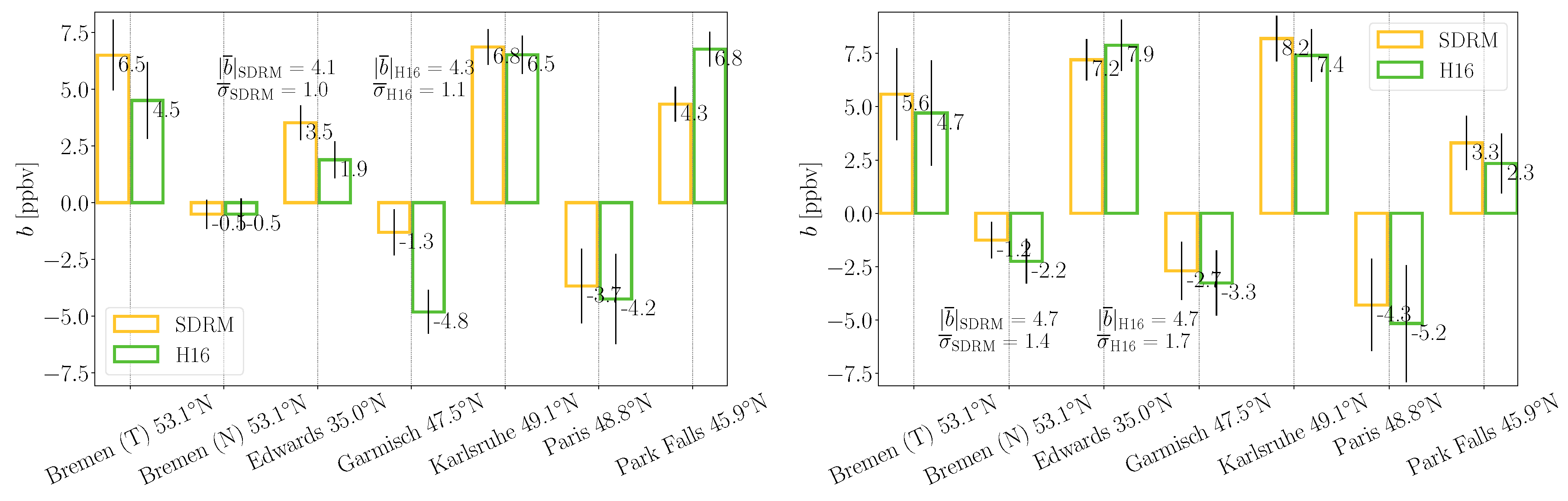
3.4. Comparison to Ground-Based Observations

In order to estimate the quality of the retrieval product, a comparison with observations from co-located TCCON (Total Column Carbon Observing Network [85,86]) and NDACC (Network for the Detection of Atmospheric Composition Change) ground-based (g-b) measurements was carried out.

Filtering of the TROPOMI retrievals is crucial in order to compare valid $\mathrm{CO}$ mole fractions to g-b references. However, it is important to note that since the errors in the retrievals are dependent on the spectroscopy, filter criteria based on errors might be appropriate for one retrieval (e.g., SDRM-based) but not the other (e.g., H16-based). The values given in

Table 2. Daily mean and median values for the SDRM- and H16-based $\mathrm{CO}$ mole fractions from TROPOMI measurements compared to Total Column Carbon Observing Network (TCCON) and Network for the Detection of Atmospheric Composition Change (NDACC) g-b observations. ‘Non-filtered’ specifies that only cloudy TROPOMI pixels were eliminated, while ‘Filtered’ additionally considers retrieval errors in the post-processing steps. ‘Radius’ designates the maximum distance for co-location, i.e., only TROPOMI observations from within that distance were compared to the g-b site. Values in brackets designate the number of observations after post-processing.

Ground-Based				TROPOMI
				Filtered			Non-Filtered
Station	Date	Mean	Median	Mean[ppbv]		Radius [km]	Median[ppbv]		Radius [km]
		[ppbv]	[ppbv]	SDRM	H16		SDRM	H16
Bremen (T)	08/05/18	86.32	86.35	92.82 (11)	90.81 (3)	50	91.93	91.05	30
Bremen (N)	11/10/18	79.77	79.82	79.26 (23)	77.29 (4)	50	78.57	77.58	20
Edwards (T)	01/07/19	85.11	87.20	88.62 (7)	86.99 (3)	50	94.40	95.07	50
Garmisch (T)	20/09/19	77.97	77.90	76.66 (6)	73.15 (4)	20	75.21	74.64	20
Karlsruhe (T)	20/09/19	77.83	78.00	84.68 (13)	84.34 (12)	15	86.19	85.40	15
Paris (T)	30/06/18	80.56	80.60	76.89 (21)	76.31 (8)	200	76.31	75.44	200
Park Falls (T)	13/06/19	77.42	77.10	81.77 (19)	84.18 (6)	150	80.40	79.44	150

are mean and median values for the respective TROPOMI overpass on the specified day. Since SDRM inferred $\mathrm{CO}$ columns exhibit smaller errors (see Section 3.2), one set of strict filter criteria leads to different numbers of observations remaining for comparison after post-processing. The actual number of remaining measurements after filtering is primarily dependent on the weather conditions at the time of overpass and surface characteristics around a station. If no TROPOMI observations remained within a reasonable small radius around the g-b station after filtering (e.g., <50 km), the radius for co-location was increased in steps of 50 km up to 200 km. The mean value was calculated for measurements that remained after strict filtering (taking retrieval errors, etc., into account), while the median was computed for the non-filtered retrieval output (i.e., only filtered for clouds). By only rejecting cloudy pixels using the S5P-NPPC product (see Section 2.2.4), both retrievals deliver the same number of $\mathrm{CO}$ mole fractions after post-processing but include observations with large errors.

The comparison to g-b reference observations in Figure 17 shows that differences vary across sites. Although no consistent over- or underestimation of BIRRA retrieved $\mathrm{CO}$ mole fractions from TROPOMI is obvious, most TCCON sites observe larger values. In accordance with results from Section 3.3, the validation shows that SDRM-based retrievals cause larger columns on average (also see Reference [59] Figure 9).

4. Discussion

4.1. Spectral Residuals

The results in Section 3.1 indicate that the SEOM line data has positive impact on the retrieval by causing significantly smaller residuals on average. Furthermore, the impact on the $\mathrm{CO}$ fitting residuals underlines results from previous studies [58] and demonstrates that improvements in spectroscopy are important, particularly for retrievals from measurements with sufficient SNR and high spectral resolution [59].

4.2. $\mathrm{CO}$ Mole Fractions

As shown in Section 3.2, the number of measurements where differences in $\mathrm{CO}$ mole fractions become significant is considerably dependent on the specific sets of line data compared. The results in Section 3.3 indicate that the increase in retrieved $\mathrm{CO}$ is within the error bar of most observations, particularly with respect to H16. Nonetheless, Figure 15 and Figure 16 also demonstrate that discrepancies can become significant over selected scenes, preferably for measurements over elevated $\mathrm{CO}$ concentrations. A comparison to Reference [59] in Figure 7 shows that $\mathrm{CO}$ retrievals from SCIAMACHY using SEOM spectroscopy also exhibit a tendency towards larger values. Moreover, the outcome in Section 3.3 indicates that the ratio of change in $\mathrm{CO}$ to its errors is roughly proportional across most geographic areas between SCIAMACHY and TROPOMI.

4.3. Validation

Since g-b observed $\mathrm{CO}$ columns can vary considerably throughout a day (>15 ppbv), representation errors, such as spatial and temporal mismatch, should be taken into account when interpreting differences for a single TROPOMI overpass. Due to advection of $\mathrm{CO}$ over time (e.g., at 3 ms${}^{-1}$), TROPOMI observations at some distance from the g-b station do also provide a valuable source of information in the comparison and should be considered, as well.

It is also important to note that TCCON data is calibrated to World Meteorological Organization (WMO) in situ trace gas measurement scales in order to tie its observations to in situ measurements [86,87]. The systematic difference between $\mathrm{CO}$ from TCCON and observations that are not tied to the WMO scale was examined in detail by Kiel et al. [88]. They found that this correction factor (1.0672 for the GGG2014 dataset) is the main source of the observed difference (also see Reference [62]) and that the choice of different spectroscopic line lists have only minor influence on the overall bias. This is in accordance with the results in Section 3.4, although different spectroscopies were compared.

5. Summary and Conclusions

The investigation on the impact of molecular spectroscopy on $\mathrm{CO}$ total columns from TROPOMI SWIR observations found that SEOM line data with the adequate model improves the spectral fit quality by reducing the residuals to TROPOMI measurements with respect to both H16 and G15.

The results demonstrate that molecular spectroscopy has a significant effect on the precision of the $\mathrm{CO}$ retrieval. The reduced spectral fitting residuals and smaller retrieval errors were found to be statistically significant across the examined regions, making the SDRM-based $\mathrm{CO}$ product more precise. The magnitude of the impact is dependent on the climatological region and spectroscopic reference but ranges from ≈ 10–20$\%$ (up to $30\%$ for individual observations with respect to G15). Updates in the ${\mathrm{H}}_2\mathrm{O}$ and ${\mathrm{CH}}_4$ cross sections were identified to be the main reason for the improved fit quality. These findings underline the important role that accurate spectroscopic information plays in meeting the missions’ requirements.

In contrast to the fitting residuals, the differences in $\mathrm{CO}$ columns between SDRM and H16 were found to be rather small across most regions ($\le 3\%$), while some larger discrepancies were found for individual observations with elevated molecular concentrations, particularly over Amazonia. Similar to the spectral residuals, the average disagreements to SDRM are larger for G15, with the largest differences to SDRM-based retrievals found over Siberia. In the other two examined regions, the impact is less significant with respect to H16 but stays significant for the majority of G15-based retrievals.

The comparison to TCCON and NDACC g-b observations revealed that the smaller retrieval errors in the SDRM inferred columns are beneficial when comparing post-processed $\mathrm{CO}$ mole fractions to g-b references since stricter filter criteria can be applied on the TROPOMI observations within a given distance from the station.

Overall, many aspects of the findings underline recommendations from earlier investigations [41,42] and are in good agreement with similar conclusions from Hochstaffl and Schreier [59].

References

1. Struve, W.S. Fundamentals of Molecular Spectroscopy; Wiley-Interscience: New York, NY, USA, 1989; p. 379. [Google Scholar]
2. Clerbaux, C.; Hadji-Lazaro, J.; Turquety, S.; Mégie, G.; Coheur, P.F. Trace gas measurements from infrared satellite for chemistry and climate applications. Atm. Chem. Phys. 2003, 3, 1495–1508. [Google Scholar] [CrossRef] [Green Version]
3. Burrows, J.P.; Platt, U.; Borrell, P. The Remote Sensing of Tropospheric Composition from Space; Physics of Earth and Space Environment; Springer: Berlin/Heidelberg, Germany, 2011. [Google Scholar] [CrossRef]
4. Veefkind, J.; Aben, I.; McMullan, K.; Förster, H.; de Vries, J.; Otter, G.; Claas, J.; Eskes, H.; de Haan, J.; Kleipool, Q.; et al. TROPOMI on the ESA Sentinel-5 Precursor: A GMES mission for global observations of the atmospheric composition for climate, air quality and ozone layer applications. Remote. Sens. Environ. 2012, 120, 70–83. [Google Scholar] [CrossRef]
5. Burrows, J.P.; Weber, M.; Buchwitz, M.; Rozanov, V.; Ladstätter-Weißenmayer, A.; Richter, A.; DeBeek, R.; Hoogen, R.; Bramstedt, K.; Eichmann, K.U.; et al. The Global Ozone Monitoring Experiment (GOME): Mission Concept and First Scientific Results. J. Atmos. Sci. 1999, 56, 151–175. [Google Scholar] [CrossRef]
6. Munro, R.; Lang, R.; Klaes, D.; Poli, G.; Retscher, C.; Lindstrot, R.; Huckle, R.; Lacan, A.; Grzegorski, M.; Holdak, A.; et al. The GOME-2 instrument on the Metop series of satellites: Instrument design, calibration, and level 1 data processing—An overview. Atmos. Meas. Tech. 2016, 9, 1279–1301. [Google Scholar] [CrossRef] [Green Version]
7. Bovensmann, H.; Burrows, J.; Buchwitz, M.; Frerick, J.; Noël, S.; Rozanov, V.; Chance, K.; Goede, A. SCIAMACHY: Mission Objectives and Measurement Mode. J. Atmos. Sci. 1999, 56, 127–150. [Google Scholar] [CrossRef] [Green Version]
8. Gottwald, M.; Bovensmann, H. (Eds.) SCIAMACHY—Exploring the Changing Earth’s Atmosphere; Springer: Dordrecht, The Netherlands, 2011. [Google Scholar] [CrossRef]
9. Levelt, P.; Oord, G.; Dobber, M.; Mälkki, A.; Visser, H.; Vries, J.; Stammes, P.; Lundell, J.; Saari, H. The Ozone Monitoring Instrument. IEEE Trans. Geosci. Remote Sens. 2006, 44, 1093–1101. [Google Scholar] [CrossRef]
10. Vonk, F. Input/Output Data Specification for the TROPOMI L01b Data Processor; Technical Report; The Royal Netherlands Meteorological Institute KNMI: Utrecht, The Netherlands, 2017. [Google Scholar]
11. Kobayashi, H. Line–by–Line Calculation using Fourier–transformed Voigt Function. J. Quant. Spectrosc. Radiat. Transfer 1999, 62, 477–483. [Google Scholar] [CrossRef]
12. Deeter, M.N.; Emmons, L.K.; Francis, G.L.; Edwards, D.P.; Gille, J.C.; Warner, J.X.; Khattatov, B.; Ziskin, D.; Lamarque, J.F.; Ho, S.P.; et al. Operational carbon monoxide retrieval algorithm and selected results for the MOPITT instrument. J. Geophys. Res. 2003, 108, 4399. [Google Scholar] [CrossRef]
13. Turquety, S.; Hadji-Lazaro, J.; Clerbaux, C.; Hauglustaine, D.; Clough, T.; Cassé, V.; Schlüssel, P.; Mégie, G. Operational trace gas retrieval algorithm for the Infrared Atmospheric Sounder Interferometer. J. Geophys. Res. 2004, 109, D21301. [Google Scholar] [CrossRef]
14. McMillan, W.; Barnet, C.; Strow, L.; Chahine, M.; McCourt, M.; Warner, J.; Novelli, P.; Korontzi, S.; Maddy, E.; Datta, S. Daily global maps of carbon monoxide from NASA’s Atmospheric Infrared Sounder. Geophys. Res. Lett. 2005, 32, L11801. [Google Scholar] [CrossRef]
15. Rinsland, C.; Luo, M.; Logan, J.; Beer, R.; Worden, H.; Worden, J.; Bowman, K.; Kulawik, S.; Rider, D.; Osterman, G.; et al. Nadir Measurements of Carbon Monoxide Distributions by the Tropospheric Emission Spectrometer onboard the Aura Spacecraft: Overview of Analysis Approach and Examples of Initial Results. Geophys. Res. Lett. 2006, 33, L22806. [Google Scholar] [CrossRef] [Green Version]
16. Lu, Y.; Khalil, M. Methane and carbon monoxide in OH chemistry: The effects of feedbacks and reservoirs generated by the reactive products. Chemosphere 1993, 26, 641–655. [Google Scholar] [CrossRef]
17. Holloway, T.; Levy, H., II; Kasibhatla, P. Global distribution of carbon monoxide. J. Geophys. Res. 2000, 105, 12123–12147. [Google Scholar] [CrossRef]
18. Feilberg, K.L.; Sellevåg, S.R.; Nielsen, C.J.; Griffith, D.W.T.; Johnson, M.S. CO + OH→CO2 + H: The relative reaction rate of five CO isotopologues. Phys. Chem. Chem. Phys. 2002, 4, 4687–4693. [Google Scholar] [CrossRef]
19. Daniel, J.S.; Solomon, S. On the climate forcing of carbon monoxide. J. Geophys. Res. 1998, 103, 13249–13260. [Google Scholar] [CrossRef]
20. Levy, H. Normal Atmosphere: Large Radical and Formaldehyde Concentrations Predicted. Science 1971, 173, 141–143. [Google Scholar] [CrossRef]
21. Crutzen, P.J.; Zimmermann, P.H. The changing photochemistry of the troposphere. Tellus A 1991, 43, 136–151. [Google Scholar] [CrossRef]
22. Buchwitz, M.; Rozanov, V.; Burrows, J. A near-infrared optimized DOAS method for the fast global retrieval of atmospheric CH4, CO, CO2, H2O, and N2O total column amounts from SCIAMACHY Envisat-1 nadir radiances. J. Geophys. Res. 2000, 105, 15231–15245. [Google Scholar] [CrossRef]
23. Buchwitz, M.; de Beek, R.; Bramstedt, K.; Noël, S.; Bovensmann, H.; Burrows, J.P. Global carbon monoxide as retrieved from SCIAMACHY by WFM-DOAS. Atm. Chem. Phys. 2004, 4, 1945–1960. [Google Scholar] [CrossRef] [Green Version]
24. Gloudemans, A.; Schrijver, H.; Hasekamp, O.; Aben, I. Error analysis for CO and CH4 total column retrievals from SCIAMACHY 2.3 μm spectra. Atm. Chem. Phys. 2008, 8, 3999–4017. [Google Scholar] [CrossRef] [Green Version]
25. Gimeno García, S.; Schreier, F.; Lichtenberg, G.; Slijkhuis, S. Near infrared nadir retrieval of vertical column densities: Methodology and application to SCIAMACHY. Atmos. Meas. Tech. 2011, 4, 2633–2657. [Google Scholar] [CrossRef] [Green Version]
26. Borsdorff, T.; Hasekamp, O.P.; Wassmann, A.; Landgraf, J. Insights into Tikhonov regularization: Application to trace gas column retrieval and the efficient calculation of total column averaging kernels. Atmos. Meas. Tech. 2014, 7, 523–535. [Google Scholar] [CrossRef] [Green Version]
27. Landgraf, J.; aan de Brugh, J.; Scheepmaker, R.A.; Borsdorff, T.; Houweling, S.; Hasekamp, O. Algorithm Theoretical Baseline Document for Sentinel-5 Precursor: Carbon Monoxide Total Column Retrieval; Technical Report; SRON Netherlands Institute for Space Research: Utrecht, The Netherlands, 2018. [Google Scholar]
28. Landgraf, J.; aan de Brugh, J.; Scheepmaker, R.; Borsdorff, T.; Hu, H.; Houweling, S.; Butz, A.; Aben, I.; Hasekamp, O. Carbon monoxide total column retrievals from TROPOMI shortwave infrared measurements. Atmos. Meas. Tech. 2016, 9, 4955–4975. [Google Scholar] [CrossRef] [Green Version]
29. Schneising, O.; Buchwitz, M.; Reuter, M.; Bovensmann, H.; Burrows, J.P.; Borsdorff, T.; Deutscher, N.M.; Feist, D.G.; Griffith, D.W.T.; Hase, F.; et al. A scientific algorithm to simultaneously retrieve carbon monoxide and methane from TROPOMI onboard Sentinel-5 Precursor. Atmos. Meas. Tech. 2019, 12, 6771–6802. [Google Scholar] [CrossRef] [Green Version]
30. Schreier, F.; Gimeno García, S.; Hochstaffl, P.; Städt, S. Py4CAtS—PYthon for Computational ATmospheric Spectroscopy. Atmosphere 2019, 10, 262. [Google Scholar] [CrossRef] [Green Version]
31. Armstrong, B. Spectrum Line Profiles: The Voigt Function. J. Quant. Spectrosc. Radiat. Transfer 1967, 7, 61–88. [Google Scholar] [CrossRef]
32. Boone, C.; Walker, K.; Bernath, P. Speed–dependent Voigt profile for water vapor in infrared remote sensing applications. J. Quant. Spectrosc. Radiat. Transfer 2007, 105, 525–532. [Google Scholar] [CrossRef]
33. Schneider, M.; Hase, F. Improving spectroscopic line parameters by means of atmospheric spectra: Theory and example for water vapor and solar absorption spectra. J. Quant. Spectrosc. Radiat. Transfer 2009, 110, 1825–1839. [Google Scholar] [CrossRef]
34. Schneider, M.; Hase, F.; Blavier, J.F.; Toon, G.; Leblanc, T. An empirical study on the importance of a speed-dependent Voigt line shape model for tropospheric water vapor profile remote sensing. J. Quant. Spectrosc. Radiat. Transfer 2011, 112, 465–474. [Google Scholar] [CrossRef]
35. Tennyson, J.; Bernath, P.; Campargue, A.; Császár, A.; Daumont, L.; Gamache, R.; Hodges, J.; Lisak, D.; Naumenko, O.; Rothman, L.; et al. Recommended isolated-line profile for representing high-resolution spectroscopic transitions (IUPAC Technical Report). Pure Appl. Chem. 2014, 86, 1931–1943. [Google Scholar] [CrossRef] [Green Version]
36. Birk, M.; Wagner, G. Voigt profile introduces optical depth dependent systematic errors—Detected in high resolution laboratory spectra of water. J. Quant. Spectrosc. Radiat. Transfer 2016, 170, 159–168. [Google Scholar] [CrossRef] [Green Version]
37. Hartmann, J.M.; Tran, H.; Armante, R.; Boulet, C.; Campargue, A.; Forget, F.; Gianfrani, L.; Gordon, I.; Guerlet, S.; Hodges, J.T. Recent advances in collisional effects on spectra of molecular gases and their practical consequences. J. Quant. Spectrosc. Radiat. Transfer 2018, 213, 178–227. [Google Scholar] [CrossRef]
38. Frankenberg, C.; Warneke, T.; Butz, A.; Aben, I.; Hase, F.; Spietz, P.; Brown, L.R. Pressure broadening in the 2ν3 band of methane and its implication on atmospheric retrievals. Atm. Chem. Phys. 2008, 8, 5061–5075. [Google Scholar] [CrossRef] [Green Version]
39. Frankenberg, C.; Bergamaschi, P.; Butz, A.; Houweling, S.; Meirink, J.F.; Notholt, J.; Petersen, A.K.; Schrijver, H.; Warneke, T.; Aben, I. Tropical methane emissions: A revised view from SCIAMACHY onboard ENVISAT. Geophys. Res. Lett. 2008, 35, L15811. [Google Scholar] [CrossRef] [Green Version]
40. Scheepmaker, R.A.; Frankenberg, C.; Galli, A.; Butz, A.; Schrijver, H.; Deutscher, N.M.; Wunch, D.; Warneke, T.; Fally, S.; Aben, I. Improved water vapour spectroscopy in the 4174–4300 cm−1 region and its impact on SCIAMACHY HDO/H2O measurements. Atmos. Meas. Tech. 2013, 6, 879–894. [Google Scholar] [CrossRef] [Green Version]
41. Galli, A.; Butz, A.; Scheepmaker, R.A.; Hasekamp, O.; Landgraf, J.; Tol, P.; Wunch, D.; Deutscher, N.M.; Toon, G.C.; Wennberg, P.O.; et al. CH4, CO, and H2O spectroscopy for the Sentinel-5 Precursor mission: An assessment with the Total Carbon Column Observing Network measurements. Atmos. Meas. Tech. 2012, 5, 1387–1398. [Google Scholar] [CrossRef] [Green Version]
42. Checa-García, R.; Landgraf, J.; Galli, A.; Hase, F.; Velazco, V.; Tran, H.; Boudon, V.; Alkemade, F.; Butz, A. Mapping spectroscopic uncertainties into prospective methane retrieval errors from Sentinel-5 and its precursor. Atmos. Meas. Tech. 2015, 8, 3617–3629. [Google Scholar] [CrossRef] [Green Version]
43. Birk, M.; Wagner, G.; Loos, J.; Mondelain, D.; Campargue, A. ESA SEOM–IAS—Measurement database—2.3 μm region [Data set]. Zenodo, 2017. Available online: https://zenodo.org/record/1009122#.X5Iw-FARVhE (accessed on 27 August 2020).
44. Birk, M.; Wagner, G.; Loos, J.; Mondelain, D.; Campargue, A. ESA SEOM–IAS—Spectroscopic parameters database—2.3 μm region [Data set]; Zenodo, 2017. Available online: https://figshare.com/articles/ESA_SEOM-IAS_Measurement_database_2_3_m_region/6632627/1 (accessed on 27 August 2020).
45. Loos, J.; Birk, M.; Wagner, G. Measurement of positions, intensities and self-broadening line shape parameters of H2O lines in the spectral ranges 1850–2280 cm−1 and 2390–4000 cm−1. J. Quant. Spectrosc. Radiat. Transfer 2017, 203, 119–132. [Google Scholar] [CrossRef] [Green Version]
46. Ngo, N.; Lisak, D.; Tran, H.; Hartmann, J.M. An isolated line-shape model to go beyond the Voigt profile in spectroscopic databases and radiative transfer codes. J. Quant. Spectrosc. Radiat. Transfer 2013, 129, 89–100. [Google Scholar] [CrossRef]
47. Ngo, N.; Lisak, D.; Tran, H.; Hartmann, J.M. Erratum to n isolated line-shape model to go beyond the Voigt profile in spectroscopic databases and radiative transfer codes [J. Quant. Spectrosc. Radiat. Transf. 129 (2013) 89 00]. J. Quant. Spectrosc. Radiat. Transfer 2014, 134, 105. [Google Scholar] [CrossRef]
48. Tran, H.; Ngo, N.; Hartmann, J.M. Efficient computation of some speed-dependent isolated line profiles. J. Quant. Spectrosc. Radiat. Transfer 2013, 129, 199–203. [Google Scholar] [CrossRef]
49. Tran, H.; Ngo, N.; Hartmann, J.M. Erratum to efficient computation of some speed-dependent isolated line profiles [J. Quant. Spectrosc. Radiat. Transfer 129 (2013) 199 03]. J. Quant. Spectrosc. Radiat. Transf. 2014, 134, 104. [Google Scholar] [CrossRef]
50. Rosenkranz, P. Shape of the 5 mm oxygen band in the atmosphere. IEEE Trans. Antennas Propag. 1975, 23, 498–506. [Google Scholar] [CrossRef]
51. Smith, E.W. Absorption and dispersion in the O2 microwave spectrum at atmospheric pressures. J. Chem. Phys. 1981, 74, 6658–6673. [Google Scholar] [CrossRef] [Green Version]
52. Dicke, R.H. The Effect of Collisions upon the Doppler Width of Spectral Lines. Phys. Rev. 1953, 89, 472–473. [Google Scholar] [CrossRef]
53. Varghese, P.; Hanson, R. Collisional narrowing effects on spectral line shapes measured at high resolution. Appl. Opt. 1984, 23, 2376–2385. [Google Scholar] [CrossRef]
54. Boone, C.; Walker, K.; Bernath, P. An efficient analytical approach for calculating line mixing in atmospheric remote sensing applications. J. Quant. Spectrosc. Radiat. Transfer 2011, 112, 980–989. [Google Scholar] [CrossRef]
55. Kochanov, V.P. Speed-dependent spectral line profile including line narrowing and mixing. J. Quant. Spectrosc. Radiat. Transfer 2016, 177, 261–268. [Google Scholar] [CrossRef]
56. Schreier, F. Computational Aspects of Speed-Dependent Voigt Profiles. J. Quant. Spectrosc. Radiat. Transfer 2017, 187, 44–53. [Google Scholar] [CrossRef] [Green Version]
57. Schreier, F.; Hochstaffl, P. Computational Aspects of Speed-Dependent Voigt and Rautian Profiles. J. Quant. Spectrosc. Radiat. Transfer 2020. In press. [Google Scholar] [CrossRef]
58. Borsdorff, T.; aan de Brugh, J.; Schneider, A.; Lorente, A.; Birk, M.; Wagner, G.; Kivi, R.; Hase, F.; Feist, D.G.; Sussmann, R.; et al. Improving the TROPOMI CO data product: Update of the spectroscopic database and destriping of single orbits. Atmos. Meas. Tech. 2019, 12, 5443–5455. [Google Scholar] [CrossRef] [Green Version]
59. Hochstaffl, P.; Schreier, F. Impact of Molecular Spectroscopy on Carbon Monoxide Abundances from SCIAMACHY. Remote Sens. 2020, 12, 1084. [Google Scholar] [CrossRef] [Green Version]
60. Gordon, I.; Rothman, L.; Hill, C.; Kochanov, R.; Tan, Y.; Bernath, P.; Birk, M.; Boudon, V.; Campargue, A.; Chance, K.; et al. The HITRAN2016 molecular spectroscopic database. J. Quant. Spectrosc. Radiat. Transfer 2017, 203, 3–69. [Google Scholar] [CrossRef]
61. Jacquinet-Husson, N.; Armante, R.; Scott, N.; Chédin, A.; Crépeau, L.; Boutammine, C.; Bouhdaoui, A.; Crevoisier, C.; Capelle, V.; Boonne, C.; et al. The 2015 edition of the GEISA spectroscopic database. J. Mol. Spectrosc. 2016, 327, 31–72. [Google Scholar] [CrossRef] [Green Version]
62. Hochstaffl, P.; Schreier, F.; Lichtenberg, G.; Gimeno García, S. Validation of Carbon Monoxide Total Column Retrievals from SCIAMACHY Observations with NDACC/TCCON Ground-Based Measurements. Remote Sens. 2018, 10, 223. [Google Scholar] [CrossRef] [Green Version]
63. Schreier, F.; Gimeno García, S.; Hedelt, P.; Hess, M.; Mendrok, J.; Vasquez, M.; Xu, J. GARLIC—A General Purpose Atmospheric Radiative Transfer Line-by-Line Infrared-Microwave Code: Implementation and Evaluation. J. Quant. Spectrosc. Radiat. Transfer 2014, 137, 29–50. [Google Scholar] [CrossRef] [Green Version]
64. Schreier, F. The Voigt and Complex Error Function: A Comparison of Computational Methods. J. Quant. Spectrosc. Radiat. Transfer 1992, 48, 743–762. [Google Scholar] [CrossRef]
65. Kleipool, Q.; Ludewig, A.; Babić, L.; Bartstra, R.; Braak, R.; Dierssen, W.; Dewitte, P.J.; Kenter, P.; Landzaat, R.; Leloux, J.; et al. Pre-launch calibration results of the TROPOMI payload on-board the Sentinel-5 Precursor satellite. Atmos. Meas. Tech. 2018, 11, 6439–6479. [Google Scholar] [CrossRef] [Green Version]
66. Van Kempen, T.A.; van Hees, R.M.; Tol, P.J.J.; Aben, I.; Hoogeveen, R.W.M. In-flight calibration and monitoring of the Tropospheric Monitoring Instrument (TROPOMI) short-wave infrared (SWIR) module. Atmos. Meas. Tech. 2019, 12, 6827–6844. [Google Scholar] [CrossRef] [Green Version]
67. Kurucz, R. Model Atmosphere Codes: ATLAS12 andATLAS9 Intensity; Harvard-Smithsonian Center for Astrophysics: Cambridge, MA, USA, 2014. [Google Scholar]
68. Van Hees, R.M.; Tol, P.J.J.; Cadot, S.; Krijger, M.; Persijn, S.T.; van Kempen, T.A.; Snel, R.; Aben, I.; Hoogeveen, W.M. Determination of the TROPOMI-SWIR instrument spectral response function. Atmos. Meas. Tech. 2018, 11, 3917–3933. [Google Scholar] [CrossRef] [Green Version]
69. Smeets, J.; Kleipool, Q.; van Hees, R.; Sneep, M. README for TROPOMI Instrument Spectral Response Functions; Technical Report; The Royal Netherlands Meteorological Institute KNMI: Utrecht, The Netherlands, 2018. [Google Scholar]
70. Golub, G.; Pereyra, V. Separable nonlinear least squares: The variable projection method and its applications. Inverse Probl. 2003, 19, R1–R26. [Google Scholar] [CrossRef]
71. Olsen, E.T.; Warner, J.; Zigang, W.; UMCP. AIRS/AMSU/HSB Version 6 CO Initial Guess Profiles (NH & SH); Technical Report; Jet Propulsion Laboratory (JPL): Pasadena, CA, USA, 2017. [Google Scholar]
72. Olsen, E.T.; Xiaozhen, X.; IMSG-NOAA/NESDIS/STAR. AIRS/AMSU/HSB Version 6 CH4 Initial Guess Profiles; Technical Report; Jet Propulsion Laboratory (JPL): Pasadena, CA, USA, 2017. [Google Scholar]
73. Hauglustaine, D.A.; Brasseur, G.; Walters, S.; Rasch, P.; Müller, J.F.; Emmons, L.; Carroll, M. MOZART: A global chemical transport model for ozone and related chemical tracers. J. Geophys. Res. 1998, 1032, 28291–28336. [Google Scholar] [CrossRef]
74. Kalnay, E.; Kanamitsu, M.; Kistler, R.; Collins, W.; Deaven, D.; Gandin, L.; Iredell, M.; Saha, S.; White, G.; Woollen, J.; et al. The NCEP/NCAR 40-Year Reanalysis Project. Bull. Am. Met. Soc. 1996, 77, 437–472. [Google Scholar] [CrossRef] [Green Version]
75. Cao, C.; De Luccia, F.J.; Xiong, X.; Wolfe, R.; Weng, F. Early On-Orbit Performance of the Visible Infrared Imaging Radiometer Suite Onboard the Suomi National Polar-Orbiting Partnership (S-NPP) Satellite. IEEE Trans. Geosci. Remote Sens. 2014, 52, 1142–1156. [Google Scholar] [CrossRef] [Green Version]
76. Cao, C.; Xiong, J.; Blonski, S.; Liu, Q.; Uprety, S.; Shao, X.; Bai, Y.; Weng, F. Suomi NPP VIIRS sensor data record verification, validation, and long-term performance monitoring. J. Geophys. Res. 2013, 118, 11664–11678. [Google Scholar] [CrossRef]
77. Siddans, R.; Smith, A. S5P-NPP Cloud Processor ATBD; Technical Report; Rutherford Appleton Laboratory (RAL): Chilton, UK, 2018. [Google Scholar]
78. Scheepmaker, R.A.; aan de Brugh, J.; Hu, H.; Borsdorff, T.; Frankenberg, C.; Risi, C.; Hasekamp, O.; Aben, I.; Landgraf, J. HDO and H2O total column retrievals from TROPOMI shortwave infrared measurements. Atmos. Meas. Tech. 2016, 9, 3921–3937. [Google Scholar] [CrossRef] [Green Version]
79. Vidot, J.; Landgraf, J.; Hasekamp, O.; Butz, A.; Galli, A.; Tol, P.; Aben, I. Carbon monoxide from shortwave infrared reflectance measurements: A new retrieval approach for clear sky and partially cloudy atmospheres. Remote. Sens. Environ. 2012, 120, 255–266. [Google Scholar] [CrossRef]
80. National Geophysical Data Center. 2-Minute Gridded Global Relief Data (ETOPO2) v2; National Geophysical Data Center, NOAA: Boulder, CO, USA, 2006. [Google Scholar]
81. Rodgers, C.; Connor, B. Intercomparison of remote sounding instruments. J. Geophys. Res. 2003, 108, 4116. [Google Scholar] [CrossRef] [Green Version]
82. Gay, D. Usage Summary for Selected Optimization Routines (PORT Mathematical Subroutine Library, Optimization Chapter); Computing Science Technical Report 153; AT&T Bell Laboratories: Murray Hill, NJ, USA, 1990; Available online: http://netlib.bell-labs.com/cm/cs/cstr/153.pdf (accessed on 17 October 2019).
83. Rust, B.W. Fitting nature’s basic functions. II. Estimating uncertainties and testing hypotheses. Comput. Sci. Eng. 2001, 3, 60–64. [Google Scholar] [CrossRef]
84. Hodges, J.L. The significance probability of the Smirnov two-sample test. Ark. Mat. 1958, 3, 469–486. [Google Scholar] [CrossRef]
85. Wunch, D.; Toon, G.C.; Blavier, J.F.L.; Washenfelder, R.A.; Notholt, J.; Connor, B.J.; Griffith, D.W.T.; Sherlock, V.; Wennberg, P.O. The Total Carbon Column Observing Network (TCCON). Philos. Trans. Roy. Soc. London Ser. A 2011, 369, 2087–2112. [Google Scholar] [CrossRef] [Green Version]
86. Wunch, D.; Toon, G.C.; Sherlock, V.; Deutscher, N.M.; Liu, C.; Feist, D.G.; Wennberg, P.O. Documentation for the 2014 TCCON Data Release. CaltechDATA 2015. [Google Scholar] [CrossRef]
87. Wunch, D.; Toon, G.C.; Wennberg, P.O.; Wofsy, S.C.; Stephens, B.B.; Fischer, M.L.; Uchino, O.; Abshire, J.B.; Bernath, P.; Biraud, S.C.; et al. Calibration of the Total Carbon Column Observing Network using aircraft profile data. Atmos. Meas. Tech. 2010, 3, 1351–1362. [Google Scholar] [CrossRef] [Green Version]
88. Kiel, M.; Hase, F.; Blumenstock, T.; Kirner, O. Comparison of XCO abundances from the Total Carbon Column Observing Network and the Network for the Detection of Atmospheric Composition Change measured in Karlsruhe. Atmos. Meas. Tech. 2016, 9, 2223–2239. [Google Scholar] [CrossRef] [Green Version]
89. Notholt, J.; Petri, C.; Warneke, T.; Deutscher, N.M.; Buschmann, M.; Weinzierl, C.; Macatangay, R.C.; Grupe, P. TCCON Data from Bremen (DE), Release GGG2014.R0. TCCON Data Archive, Hosted by CaltechDATA. 2014. Available online: https://data.caltech.edu/records/268 (accessed on 27 August 2020).
90. Iraci, L.T.; Podolske, J.; Hillyard, P.W.; Roehl, C.; Wennberg, P.O.; Blavier, J.F.; Allen, N.; Wunch, D.; Osterman, G.; Albertson, R. TCCON Data from Edwards (US), Release GGG2014.R1. TCCON Data Archive, Hosted by CaltechDATA. 2016. Available online: https://data.caltech.edu/records/268 (accessed on 27 August 2020).
91. Sussmann, R.; Rettinger, M. TCCON Data from Garmisch (DE), Release GGG2014.R2. TCCON Data Archive, Hosted by CaltechDATA. 2018. Available online: https://data.caltech.edu/records/268 (accessed on 27 August 2020).
92. Hase, F.; Blumenstock, T.; Dohe, S.; Gross, J.; Kiel, M. TCCON Data from Karlsruhe (DE), Release GGG2014.R1. TCCON Data Archive, Hosted by CaltechDATA. 2015. Available online: https://data.caltech.edu/records/268 (accessed on 27 August 2020).
93. Té, Y.; Jeseck, P.; Janssen, C. TCCON Data from Paris (FR), Release GGG2014.R0. TCCON Data Archive, Hosted by CaltechDATA. 2014. Available online: https://data.caltech.edu/records/268 (accessed on 27 August 2020).
94. Wennberg, P.O.; Roehl, C.M.; Wunch, D.; Toon, G.C.; Blavier, J.F.; Washenfelder, R.; Keppel-Aleks, G.; Allen, N.T.; Ayers, J. TCCON data from Park Falls (US), Release GGG2014.R1. TCCON Data Archive, Hosted by CaltechDATA. 2017. Available online: https://data.caltech.edu/records/268 (accessed on 27 August 2020).
Figure 1. Spectral transmittance of CO , CH 4 and H 2 O (upper three panels) according to Beer-Lambert’s law in spectral range of TROPOMI’s band 7 for a single path through the US-Standard atmosphere using Scientific Exploitation of Operational Missions (SEOM) line data. The total transmission for the three molecules is depicted in the lower panel. The Python tool Py4CAtS (Python for Computational ATmospheric Spectroscopy [30]) was used to calculate the absorption cross sections of the individual molecules. Note that CO is only responsible for 1 % of the total optical thickness τ in that spectral range.
Remotesensing 12 03486 g001
Figure 2. SDRM and Voigt (VGT) molecular cross sections for CO (left), CH 4 (center), and H 2 O (right) using SEOM data. In addition, the difference between the two line profiles (SDRM-VGT) is depicted.
Remotesensing 12 03486 g002
Figure 3. A calibrated level 1b photon radiance and irradiance spectrum from TROPOMI’s band 7 with SI (Système international d’unités) units mol s 1 m 2 nm 1 and the retrieval window indicated in gray (top). The Earth radiance I was obtained in orbit 9093 at around 60 northern latitude, while the solar irradiance E was measured in orbit 9088. The lower panel depicts the retrieval window from 4277.20–4302.90 cm 1 with units converted to W m 2 nm 1 . E Kurucz and E Planck 5777 describe the incident solar irradiance at TOA (top of atmosphere) according to Kurucz [67] and an equivalent black body radiator at 5777 K, respectively. Both were added for illustrative purpose only.
Remotesensing 12 03486 g003
Figure 4. Distribution of the maximum normalized amplitudes (left) and corresponding full-width at half maxima (FWHM) (right) for the 24 × 256 tabulated responses [69].
Remotesensing 12 03486 g004
Figure 5. Tabulated responses for ground pixel 128 (out of 256) in TROPOMI’s band 7. The instrument spectral response functions (ISRFs) are normalized + S i j ( x ) d x = 1 in the wavelength ( x = λ ) and wavenumber ( x = ν ) domain, respectively.
Remotesensing 12 03486 g005
Figure 6. Initial guess mole fraction profiles for CO (four panels on the left) and CH 4 (right) resembling the Atmospheric Infrared Sounder (AIRS) version 6 first guess. The CO profiles are provided with monthly granularity for both hemispheres while only January, April, July and October (clockwise from top-left) are shown here.
Remotesensing 12 03486 g006
Figure 7. Altitude sensitivity of the CO retrieval in the 4277.20–4302.90 cm 1 spectral range. The column averaging kernels (CAKs) were calculated for different TROPOMI observer zenith angles (OZAs) with a solar zenith angle (SZA) of 30 and a surface albedo of r 0 = 0.3 .
Remotesensing 12 03486 g007
Figure 8. Distribution of the elements of the residual vectors for a single overpass per season in 2019 (Table 1). The histograms are shown per region, i.e. Sahara (top-left), Central-Europe (top-right), Amazonia (lower-left), and Siberia (lower-right). VGT represents cases for which the Voigt profile was calculated with SEOM line data input (SEOM-Voigt).
Remotesensing 12 03486 g008
Figure 9. Spectral residuals for a measurement over the Sahara, Central-Europe, Amazonia, and Siberia (from top to bottom) in spring 2019, respectively. The observations were randomly picked; however, the largest disagreements appear to be at similar wavenumbers across the different regions, most prominent close to 4295 cm 1 and particularly pronounced in the fits with the two Voigt spectroscopies.
Remotesensing 12 03486 g009
Figure 10. Spectral fitting residuals for TROPOMI observations in the four regions (same order top to bottom as in Figure 9) from the earlier mentioned subset in 2019. Large residuals in the upper four panels reveal to be co-located with strong (and overlapping) absorption lines depicted in the lower three panels. However, similar to Figure 9, the overlapping transitions close to 4295 cm 1 causes rather less significant fitting errors in the SDRM retrievals. Moreover, compared to H16, the average fitting residual is smaller for SDRM in all of the examined regions.
Remotesensing 12 03486 g010
Figure 11. Distribution of retrieved quantities for Sahara. The CO columns and corresponding errors for different spectroscopic inputs and models are shown in the top-row. Histograms for the co-retrieved CH 4 and H 2 O columns are depicted in the two panels below. The median of each distribution is shown in the corresponding color.
Remotesensing 12 03486 g011
Figure 12. Distribution of the retrieved values and errors for Central-Europe.
Remotesensing 12 03486 g012
Figure 13. Distribution for the Amazonia region which include an overpass during the heavy forest fires in summer 2019 (orbit 9553 on 17 August 2019).
Remotesensing 12 03486 g013
Figure 14. Distributions over Siberia.
Remotesensing 12 03486 g014
Figure 15. Differences in the retrieved CO mole fractions as a function of the CO concentrations over Amazonia (top) and Central-Europe (bottom).
Remotesensing 12 03486 g015
Figure 16. CO mole fractions (left column) and errors (center column) for SDRM-based retrievals, along with differences between SDRM and H16 (SDRM-H16) over Amazonia (top-row) and Central-Europe (bottom-row).
Remotesensing 12 03486 g016
Figure 17. Differences of TROPOMI and TCCON/NDACC mean (left) and median (right) CO mole fractions from Table 2. Note that the mean was calculated upon the strictly filtered retrieval output, while the median includes all cloud-free retrievals.
Remotesensing 12 03486 g017