Abstract
Synthetic aperture radar (SAR) images contain severe speckle noise and weak texture, which are unsuitable for visual interpretation. Many studies have been undertaken so far toward exploring the use of SAR-to-optical image translation to obtain near optical representations. However, how to evaluate the translation quality is a challenge. In this paper, we combine image quality assessment (IQA) with SAR-to-optical image translation to pursue a suitable evaluation approach. Firstly, several machine-learning baselines for SAR-to-optical image translation are established and evaluated. Then, extensive comparisons of perceptual IQA models are performed in terms of their use as objective functions for the optimization of image restoration. In order to study feature extraction of the images translated from SAR to optical modes, an application in scene classification is presented. Finally, the attributes of the translated image representations are evaluated using visual inspection and the proposed IQA methods.
1. Introduction
Synthetic aperture radar (SAR) remote sensing is an effective means of Earth observation and plays an important role in scene monitoring, situation recording and change detection [1]. It collects data in a reliable way, as the microwave band electromagnetic waves are robust to various weather and geographical environments. However, SAR images have different characteristics from optical images and are not suitable for visual interpretation. On the one hand, speckle noise in SAR images widely exists due to the coherent summation of signal responses from individual scatterers in resolution cells [2]. High-frequency noise affects the detection of features and makes images difficult to be recognized by humans. On the other hand, SAR images inherently contain geometric distortion, which is caused by the distance-dependence along the range axis and the characteristics of radar signal wavelengths [1]. Humans are accustomed to the visible part of the electromagnetic spectrum. Thus, difficulties in distinguishing structural information of SAR images remain to be solved in spite of increasing spatial resolution.
In recent years, many methods have been proposed to use generative adversarial networks (GANs) for SAR-to-optical image translation [3,4,5,6]. Scholars believe that the interpretation of SAR images can be made easier if we convert them into optical representations. As a result, the models used in the field of image-to-image translation have played an active role, including supervised and unsupervised architectures [7,8,9,10]. However, there is no universally accepted method for the evaluation of SAR-to-optical image translation. Expert evaluation is often used as visual inspection but is subjective in most cases. Traditional image quality assessment (IQA) measures were considered as references [10,11], but the availability of the objective metrics for the stylization tasks has not been explored, along with the abilities to identify the differences between the generated images and carry out appropriate feature recognition. As a new evaluation of model performance, [1] introduced a road segmentation method to study the consistency of the aspect ratio of objects in the process of translation. However, this is limited to the images with line features.
The effectiveness of SAR-to-optical image translation depends not only on the selection of translation models, but also the means of quality assessment. Based on [12], IQA methods have two purposes: one is to objectively evaluate the quality of the results generated by different models, and the other is to guide the optimization of network architectures and algorithms, which is widely used in image restoration [13], video coding [14] and image analysis [15]. In this paper, we design an image restoration approach to explore different IQA metrics. Inspired by Ding et al. [16], who evaluated 11 full-reference IQA models for image processing systems, we build a deep convolution neural network. Through optimization, the network can restore various distorted images with the capabilities to recognize different regions of interest in the images. Our attention focuses on image correction, deblurring and denoising in this work.
Thus, this paper is concerned with image quality assessment for SAR-to-optical image translation, and can be regarded as a closed-loop system, shown in Figure 1. Firstly, four image-to-image translation models are adopted as baselines to transform images from SAR to optical modes. Then, translation results and distorted images pass to the image restoration model, where attributes of the perceptual IQA models are systematically demonstrated and compared. To analyze the consistency of multiple features in the progress of translation, a scene classification scheme is presented. Finally, translation results are evaluated based on feedback from visual inspection and IQA methods. This work is image-to-image translation from single-channel SAR images to single-channel optical images, so the optical data are converted to gray scale in advance. Specifically, the major contributions of this paper are as follows:

Figure 1.
The framework of our algorithm.
- In view of the difficulties in the interpretation of SAR images, a SAR-to-optical image translation model is designed, which realizes the translation by taking advantage of the baselines containing supervised and unsupervised architectures.
- Considering the lack of quality assessment tools in SAR-to-optical image translation, a large-scale comparison of perceptual IQA models is performed to select suitable ones and explore the availability of objective metrics for stylization tasks.
- Besides visual perception and IQA measures, the properties of the translation results in terms of follow-up applications are described. We launch discussion and evaluation of scene classification in this paper to ensure the diversity of features involved.
2. Related Works
2.1. Image-to-Image Translation
Similar to automated language translation, the image-to-image translation task is to transform one representation into another [17]. Conditional generative adversarial networks (cGANs) are a suitable option for tackling image-to-image translation tasks due to their properties to generate images based on two references, one for content and one for style [1]. In 2016, Isola et al., put forward a framework which transforms images from pixel to pixel (pix2pix) [7] for image-to-image translation. It is based on cGANs and U-Net architectures. However, it needs paired training data, which is not available for many tasks. Subsequently, a circular consistent method, namely CycleGAN [8], was proposed by Zhu et al., to perform unsupervised translation with unpaired images. It can translate an image from a source domain to a target domain in the absence of paired examples, whereas the results are often limited to low resolution. The unsupervised framework was applied to SAR-to-optical translation, which indicated a promising potential to support SAR image interpretation [1]. In 2018, Wang et al., introduced a high-resolution framework pix2pixHD [9] with multi-scale generator and discriminator architectures, and generated 2048 × 1024 visually appealing results. Considering that the previous studies had been limited to the spatial domain, feature-guided SAR-to-optical image translation (FGGAN) [10] added certain loss in the process of discrete cosine transformation (DCT) to ensure consistency in the frequency domain. Image to image translation has been widely used in style transfer, object transfiguration, season transfer photo enhancement, etc. Similar ideas have been applied to various tasks such as generating photographs from sketches and transforming Google maps to satellite views. In our current paper, the above models are adopted and optimized to translate SAR images to optical images. Since SAR is geometrically accurate, we take advantage of the rich content in SAR images and use the style from the optical side. Performance of different models in terms of SAR-to-optical image translation are tested on multiple scenes.
2.2. Image Quality Assessment (IQA)
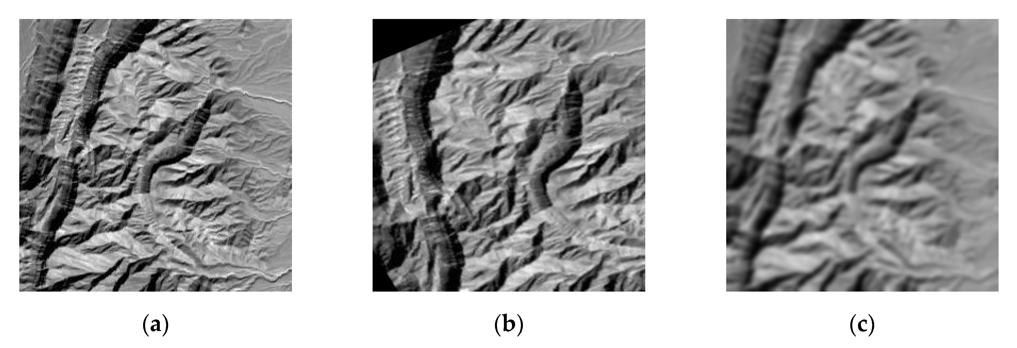
Reasonable evaluation means are beneficial to system improvement, help to optimize the established algorithms, and reduce the cost of visual assessment. Mean square errors (MSE) [18] had been used in the field of full-reference evaluation for over 50 years but were criticized for poor correlation with human perception [19]. Then, a series of IQA methods aimed at perceptual optimization were proposed. Structural similarity (SSIM) [20] takes the brightness and contrast related to the object structure as the information of an image, whereas the weights of each pixel are given as the same, which is not consistent with the characteristics of images. For example, when we define the structure of an object, the pixels on the edge are more important than those in the background areas. Thus, feature similarity (FSIM) [21] focuses on attaching appropriate importance to the pixels of an image. However, SSIM, FSIM and MSE rely too much on the full alignment between image pixels, resulting in their high sensitivity to the differences between two images of the same texture, such as two different areas of the same grassland [22]. In addition, we find that they are vulnerable to different angles of the same view obtained by sensors. Figure 2 shows IQA scores between the original and the distorted images. Warp affine looks more similar to the original one than Gaussian blur by human perception. But MSE and SSIM give a different result. Human evaluation of similarity depends on a high-order image structure [23]. It is also context-sensitive [24], so there is not a strict formula for similarity measure. Driven by the surge of convolutional neural networks (CNN), Zhang et al., proposed learned perceptual image patch similarity (LPIPS) [25] in 2018, using the features extracted from specific convolution layers of the visual geometry group (VGG) network [26] as the feature-matching loss. This takes high-level semantic information as guidance and bridges the gap between scientific metrics and perceptual measurements (see Figure 2). In 2020, Ding et al., introduced a method named deep image structure and texture similarity (DISTS) [22] by combining structural similarity with texture similarity, which not only correlates well with human perception, but also achieves a high degree of invariance to texture substitution. Suitable IQA measurements contribute to the assessment of translation performance, comparison of translation systems, and visual quality improvement.
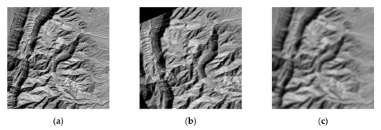
Figure 2.
A single channel remote sensing image of mountain. (a) Original image, (b) same view, distorted by warp affine, and (c) same view, distorted by Gaussian blur. Image quality assessment (IQA) scores between (a) and (b): mean square error (MSE) = 0.091, structural similarity (SSIM) = 0.056 and learned perceptual image patch similarity (LPIPS) = 0.628. IQA scores between (a) and (c): MSE = 0.009, SSIM = 0.537 and LPIPS = 0.661. (Note that, unlike MSE and LPIPS, larger values of SSIM indicate better quality.).
2.3. Image Feature Extraction
In this paper, to explore the impact of the generated images on feature extraction, an image classification strategy is implemented. Since CNN is good at calculating and extracting features that are used as the input of classifiers, we assess the performance of feature extraction and implement image classification by deploying full connection and softmax layers to classify the features extracted by CNNs. With the rapid development of CNN, a variety of networks such as VGG [26], SqueezeNet [27], ResNet [28], and Inception [29] have emerged in recent years. VGG is introduced by Simonyan et al., and achieves 92.7%, the top-5 test accuracy, in the ImageNet classification experiment. However, it has a large number of parameters. SqueezeNet is aimed at reducing the computational cost and improving the running speed without affecting the classification accuracy. It achieves results similar to AlexNet [30] and reduces the parameters by 50 times simultaneously. Nevertheless, vanishing and exploding gradients will occur when the network goes deeper, even though a deeper network brings better results to a certain degree. ResNet is put forward by Kaiming et al., and uses shortcut connections to solve the problems of vanishing and exploding gradients. Meanwhile, Inception uses a dense component to replace the optimal local sparse structure and realizes the feature fusion of different scales. As an important attribute of images, the most discriminative features help us distinguish different images. The classification results are effective to detect the feature extraction ability of different networks and explore the impact of SAR-to-optical image translation on the image features.
3. Methods
3.1. Synthetic Aperture Radar (SAR)-to-Optical Image Translation Model
3.1.1. Network Architectures
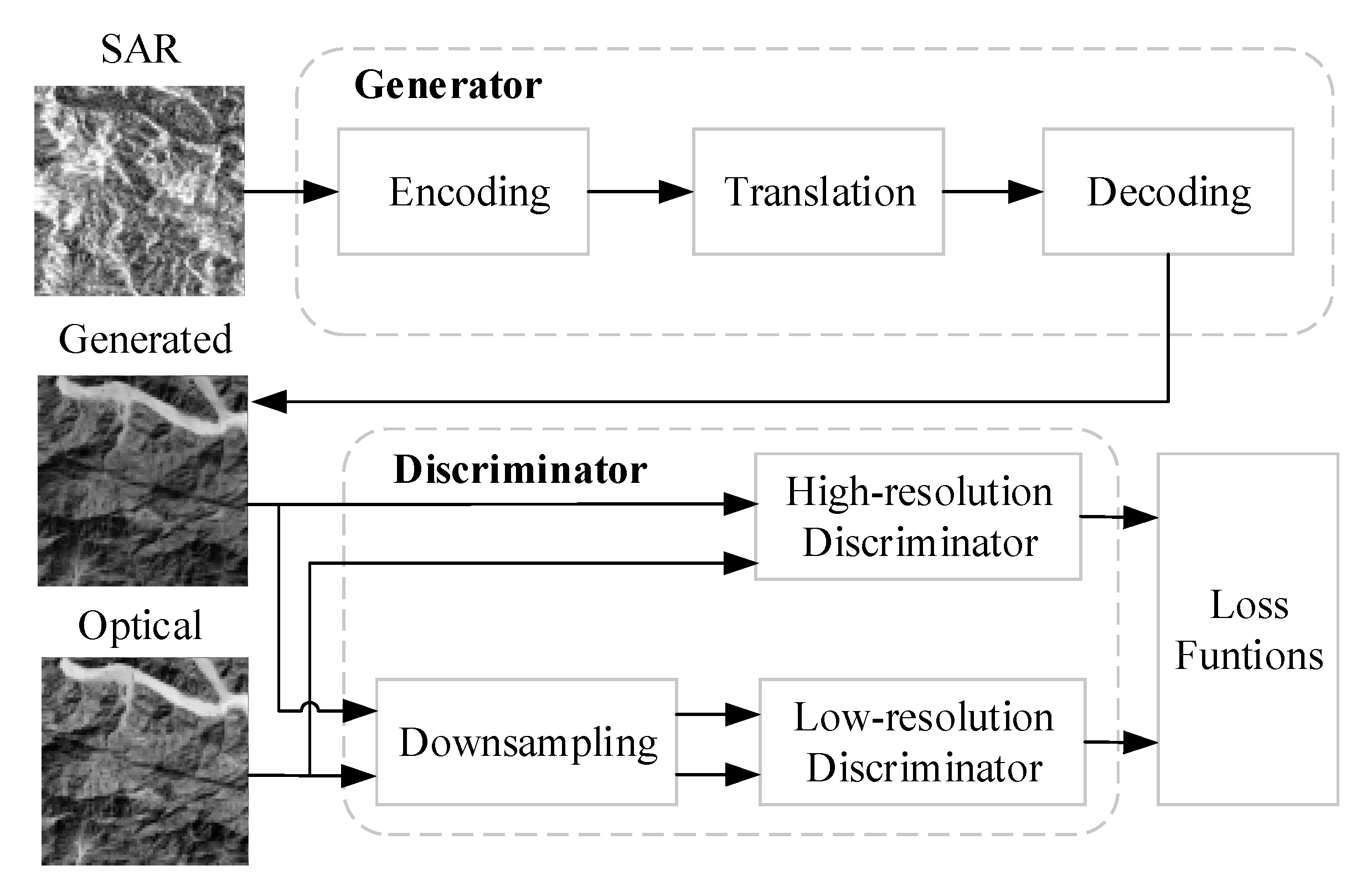
Inspired by the standard image-to-image translation network, which is composed of encoding, translation and decoding parts, our network structure is divided into three modules shown in Figure 3. These modules are: SAR image feature encoding, SAR-to-optical translation, and optical image decoding. The SAR image feature encoding module obtains the coding expression of SAR images and extracts their high-level semantic information through down-sampling of multiple convolutional layers. The SAR-to-optical translation module achieves the translation of encoding tensors from SAR to optical modes. The decoding module uses a de-convolution structure to up-sample the encoding tensors and then convert them into normal optical images with the same size as input SAR images. The generated images and real optical images are put into the discriminator together, which needs to be sampled if using multi-scale discriminators. The multi-scale discriminator uses two discriminators with different resolutions of image input but the same network architecture. They are called high-resolution and low-resolution discriminators, shown in Figure 3, which not only pay attention to high-level global information of images and ensure a large receptive field, but also focus on low-level details. In this work, the real optical images and the generated optical images are down-sampled with a coefficient of 2 to create image pyramids with two scales. For example, if generating images with the size of 256 × 256 with 1/2 down-sampling, the input size is 256 × 256 and 128 × 128, respectively. Finally, loss functions are applied with gradient descent and backpropagation to implement the adversarial game between the generator and the discriminator.

Figure 3.
Architectures of the proposed synthetic aperture radar (SAR)-to-optical image translation model.
Baselines adopted here are Pix2pix [7], CycleGAN [8], Pix2pixHD [9] and FGGAN [10]. Pix2pix and CycleGAN both use U-Net [7] on the generator and skip connections between the encoding and decoding layers, which help us to share information between different levels. Pix2pixHD and FGGAN use multi-scale discriminators, averaging the results of the original image, 1/2 down-sampling and 1/4 down-sampling. To extract the high-frequency features, we apply PatchGAN [7] which effectively models images as Markov random fields [10]. It does not need to send the whole image into the discriminator, but we give the binary decision i.e., true or false to each patch with the size of N × N, and take the average of the results as the final output. The patch size N denotes the receptive fields of our discriminator. The effects of varying N from a 1 × 1 “PixelGAN” to a full 256 × 256 “ImageGAN” are tested by adjusting the depth of the GAN discriminator. Inspired by Pix2pix [7], which shows that the 70 × 70 “PatchGAN” can alleviate tiling artifacts and achieve better fully convolutional network (FCN) scores, we set the patch size N to 70 in the balance of computational costs and image quality. Different patches are regarded independent of each other.
3.1.2. Loss Functions
GANs pursue a minimax game between the generator and the discriminator, where the loss function is an important part to balance the two modules. For our task, the objective of the generator is to translate initial SAR images to near-optical representations, while the discriminator aims to distinguish the actual optical images from the translated ones:
where is the generator, denotes the discriminator, and is the loss function of each translation model. and represent the generator and discriminator, respectively, when reaches the minimum.
- Pix2pix
Pix2pix [7] not only uses adversarial losses to construct the details of the high frequency part, but also introduces norm to drive the generated images to approach the reference at low frequencies:
where determines the weight of loss . and are given by
where and are the input and output images respectively.
- CycleGAN
CycleGAN [8] presents a cycle consistency loss, which is essentially the loss between the original image and its translated version. In order to realize the translation circle of the two domains, it contains two adversarial losses:
where and represent the first and the second image domains respectively. The first adversarial loss is from to , where is the generator, and is the discriminator. The second one is from to , where is the generator, and is the discriminator. is the cycle consistency loss whose importance is determined by :
- Pix2pixHD
Pix2pixHD [9] introduces the Max function in order to optimize the maximum loss under three different scales of the discriminators. Meanwhile, a feature-matching constraint is added to calculate losses in the progress of feature extraction:
where denotes the number of the discriminators. stands for the feature matching loss which is weighted by . It is expressed as follows:
where is the total number of the layers for feature extraction, which are the ReLU layers in front of each max-pooling layer in the VGG—19 network. So is set to 5 experimentally. , and denote the height, width and channel of the feature maps respectively.
- FGGAN
FGGAN [10] considers the unification of the spatial and frequency domains:
where is the VGG loss, and is the Discrete Cosine Transform loss. Their weights are determined by and respectively. inspired by in pix2pixHD uses norm, because the model does not pursue sparsity or have problems of fuzzy edges. Interestingly, experiments show that if DCT uses norm, it will be degenerated into the same gradient as that of the original image, which leads to image blur. Therefore, norm is used in the DCT model:
3.2. Image Restoration Model
The way to prove the availability of IQA metrics for the stylization tasks is to detect the influence of the metrics on the image-processing algorithms. We assume that there is an ideal optical image, whose view is identical to the SAR image. The optical image converted from a SAR image can be regarded as the result of an image restoration procedure. To simplify the process, we restore the generated and distorted images in this section.
3.2.1. Network Architectures
The image restoration structure is designed according to enhanced deep residual networks for single image super-resolution (EDSR) [31], which was originally used to deal with super-resolution images. It is chosen as the base because super-resolution problems have physical connections with the tasks involved in this paper.
Single image super-resolution aims to enhance the resolution and quality of a low-resolution image [16]. When there is an original image and an observed image , we model their relationship as:
where denotes down-sampling which is an ill-posed problem because down-sampling is a projection onto a low-dimensional subspace. is a spatially varying linear kernel and is the noise incorporated in the process.
Our tasks are regarded as image correction, deblurring and denoising. The distortions come from the failure cases of translation, filtering and noise removal, which have no change in resolution. Thus, the distorted images can be expressed as follows:
It does not have down-sampling parameters but involves spatial variation and noise integration. As a result, the architecture of the image restoration network is designed without any up-sampling part. As shown in Figure 4, batch normalization is also eliminated to stack more layers and ensure better performance.

Figure 4.
Architecture of the distorted image restoration model. It includes 16 residual blocks. 3 × 3 Conv. indicates the convolutional kernel with the size of 3 × 3. The number after the dot represents the output channel of each convolutional layer.
3.2.2. Loss Functions
We choose SSIM, FSIM, MSE, LPIPS, and DISTS as preparatory metrics. In the task of image restoration, the goal is to restore an observed image close to the original one via the guidance of the IQA methods. Metrics are applied to the loss functions in the image processing algorithm.
where represents a full-reference quality assessment metric and is the image recovered from the distorted one . In this work, stands for the distance between and under each metric, and uses the least-square method if IQA is not involved. The aim of the algorithm is to minimize and obtain the restoration result closest to the reference image.
In the process of the Deep Neural Networks (DNN) mapping, the network is trained to estimate noise involved in the distortion. It is subtracted in the loss function. Thus, the model is optimized by the norm:
where is the parameterized DNN mapping, and can be regarded as used in Equation (13).
Note that unlike MSE, LPIPS and DISTS, larger values of SSIM and FSIM indicate better quality. Because the values of SSIM and FSIM fall in the range of (0,1), an additional process of (1—value) is performed when they are substituted into the loss function.
4. Experiments
4.1. Datasets
In this paper, three datasets for different tasks are obtained by random sampling from the “SEN1-2 dataset” provided by Schmitt et al. [32]: Image Translation Dataset, Image Restoration Dataset, and Image Classification Dataset. The “SEN1-2 dataset” is derived from (1) the European Space Agency (ESA)’s Sentinel-1 C-Band SAR using the ground-range detected (GRD) product, collected in the interferometric wide swath (IW) mode, and constrained to Vertical–Vertical (VV) polarity; and (2) ESA’s Sentinel-2 multi-spectral imagery constrained to bands 4, 3, and 2 (red, green, and blue channels).
The Image Translation Dataset consists of pairs of “SAR-optical” images, which cover five categories of scene: Farmland, Forest, Gorge, River and Residential. We think these five types of scene are representative of SAR-based remote-sensing observations, as they have very different features. The classification depends on our investigation of a large number of remote-sensing datasets, which are presented in Appendix A Table A1.
The Image Restoration Dataset includes two types of distortions in optical images: GAN and traditional distortions. GAN distortion contains the cases generated by the translation models, while traditional distortion is manually made by us, which consists of contrast shift, Gaussian blur and speckle noise. When an image arrives, the tool responsible for contrast shift converts it to . The Gaussian kernel size is set to 11 × 11, and the variance of speckle noise is 0.2.
The Image Classification Dataset is made up of the images generated by the translation models, so the scenes processed in the classification experiments are the same as those of the Image Translation Dataset. Specific numbers of each dataset are tabulated in Table 1.

Table 1.
The information of images involved in the Image Translation, Image Restoration, and Image Classification Datasets. Values in the parentheses represent the specific number of images in each category.
It is worth mentioning that the initial object of our tasks is spaceborne SAR, which provides single channel images. Translation from single channel SAR images to multi-channel optical images is an ill-posed problem, just like the colorization of gray-scale images in the classical computer vision [33]. So the original optical images are grayed in advance in this paper, using a weighted average method.
4.2. Implement Details
Experiments involved in this paper were implemented on PyTorch and the computing platform was a single RTX TITAN graphics processing unit (GPU) with a 24 GB GPU memory. The inputs in the image translation experiment are single-channel images with the dimension of 256 × 256 × 1, which are the same as that of the generated images used in image restoration and scene classification. The parentheses indicate the parameters of the Adam optimizer, and imply the momentum when using stochastic gradient descent (SGD). The Learning Rate (LR) of the translation model is set to 0.0002 initially, then decreases linearly to 0 in the last 50 epochs of pix2pix/CycleGAN and the last 100 epochs of pix2pixHD/FGGAN. The LR of the image restoration model remains at a fixed value of 0.005 in the first 2000 iterations, which decays linearly by a factor of 2 for every 2000 iterations subsequently. In the image classification experiment, we set 50 epochs before over fitting appears. Learning rate is fixed at 0.001. Specific experimental parameters are shown in Table 2.

Table 2.
Parameters involved in the process of Image Translation, Image Restoration, and Image Classification.
4.3. Visual Inspection of SAR-to-Optical Translation
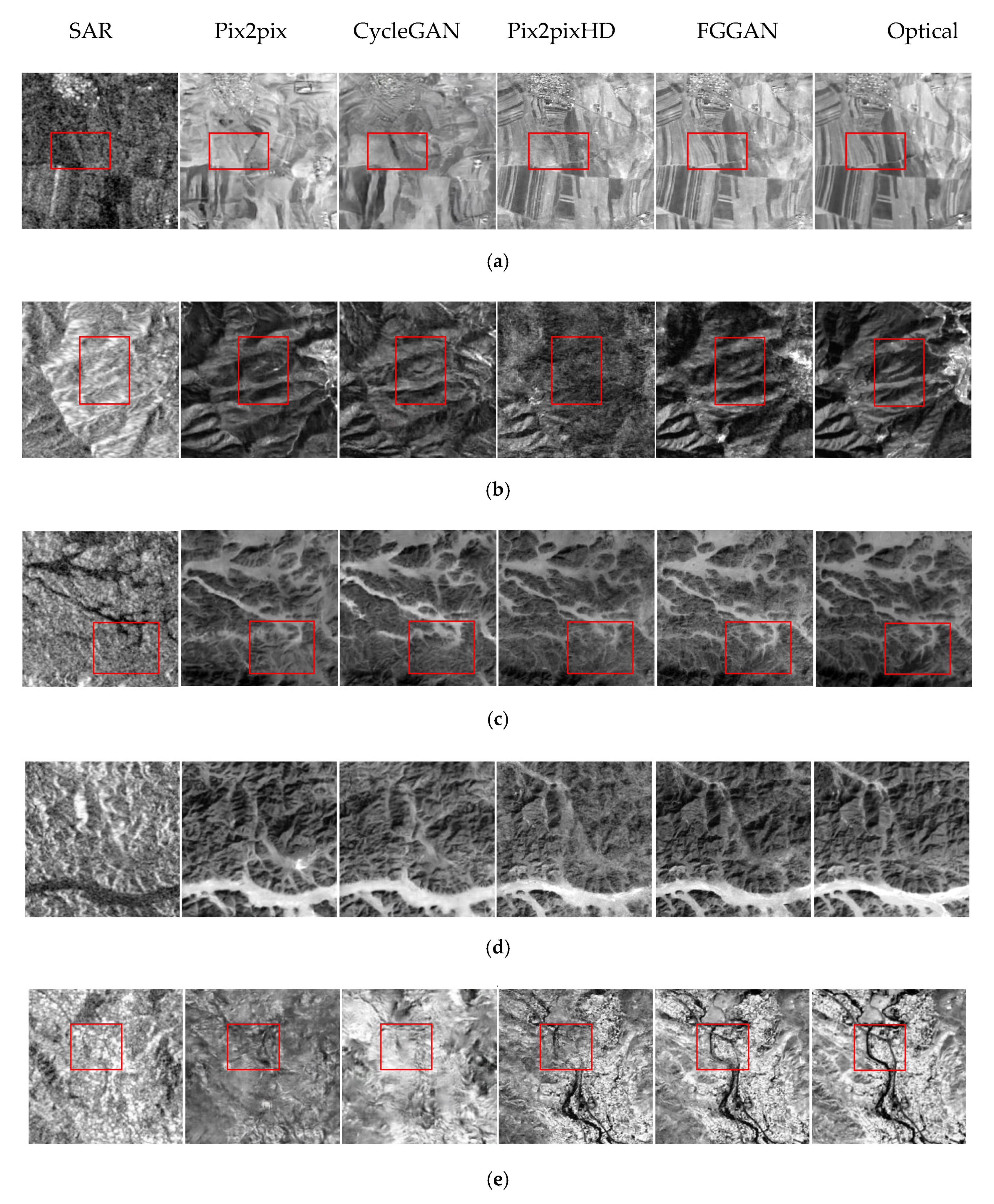
As shown in Figure 5, four end-to-end image translation models: pix2pix, CycleGAN, pix2pixHD and FGGAN, along with five categories of scene: Farmland, Forest, Gorge, River and Residential are involved in the experiment. The first column consists of the original SAR images, which are the input of the translation models. On the right-hand column are optical images, with which the generated images in the middle columns are compared. The red rectangles in the images highlight the details of the translation results, which do not set restrictions on the reader’s attention but can be used as a guidance for visual perception to some extent. The evaluation method takes into account the geometric accuracy and texture characteristics of the translated images. Various scenes provide guarantee for detecting the generalization performance of the models, and pave the way for the subsequent multi-classification task.
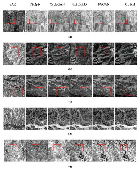
Figure 5.
Multiple scenes image translation results obtained by pixel to pixel (pix2pix), cycle-consistent adversarial networks (CycleGAN), high-definition pixel to pixel (pix2pixHD) and feature-guided SAR-to-optical image translation (FGGAN). (a) Farmland, (b) Forest, (c) Gorge, (d) River, and (e) Residential.
- Farmland
Divisions between blocks are the most important elements in Farmland, followed by the shade of the gray regions in each block, which are caused by different crops. Such features are often submerged by speckle noise and difficult to recognize in the SAR images. From Figure 5a, we can see that images generated by pix2pix and CycleGAN largely differ from the optical ones. Only several blocks of different crops, which appear with different shades of the gray regions in the optical image, are presented, while the segmentations are not restored. Results of pix2pixHD and FGGAN are greatly improved except for the area in the red rectangle. As farmland is a man-made scene and is not far away from the residential areas, it is necessary to distinguish them when meeting the transition from farmland to urban and rural areas. Such translation results in more detailed information are shown in Figure A1.
- Forest
Attention should be focused on the depth of the texture in Forest. As shown in Figure 5b, complex interlaced textures are presented over the whole image. Although CycleGAN is good at extracting features and generating redundant content, it is not accurate. In the red rectangle, we find that Pix2pixHD does not perform well in feature extraction of texture with different brightness, as well as concave and convex texture.
- Gorge
Gorge in this paper refers to a valley with the steep slope, whose depth is far greater than its width, and a lake with natural vegetation. Due to the steep slope, the flow is turbulent and rocks of various shapes are formed in the water. The contour of the vegetation along the shore is also involved, which constitutes a challenge for feature extraction. From Figure 5c, we can see that the translation results of gorge are generally consistent with those of the optical ones, except for some details of the shore. For example, the red rectangle shows the impact on the coastal land due to the slope and river erosion, which needs to be further processed.
- River
We shall pay attention to the outline and direction of the River, as well as the tributaries scattered from the main river course. In Figure 5d, the main trend of the river is generally restored. However, the translation results of the sparsely vegetated area need to be improved.
- Residential
Residential areas belong to a complex scene with buildings, road traffic and other man-made structures, with obvious point and line features [1]. Current image translation works are still limited to the integration of the residential areas. Just as trees in the forest cannot be subdivided, buildings and structures in the Residential areas cannot be distinguished. In Figure 5e, point features such as residential buildings are difficult to recognize in the SAR images, affecting the translation of pix2pix and CycleGAN. Meanwhile, the red rectangle shows that pix2pixHD and FGGAN have difficulties in detecting the road features.
Generally speaking, pix2pix and CycleGAN mainly focus on contextual semantic information in multiple scenes of SAR-to-optical image translation, at the cost of ignoring local information. Pix2pixHD and FGGAN can extract and express features more comprehensively, paying more attention to details while grasping the overall semantics.
4.4. IQA Model Selection
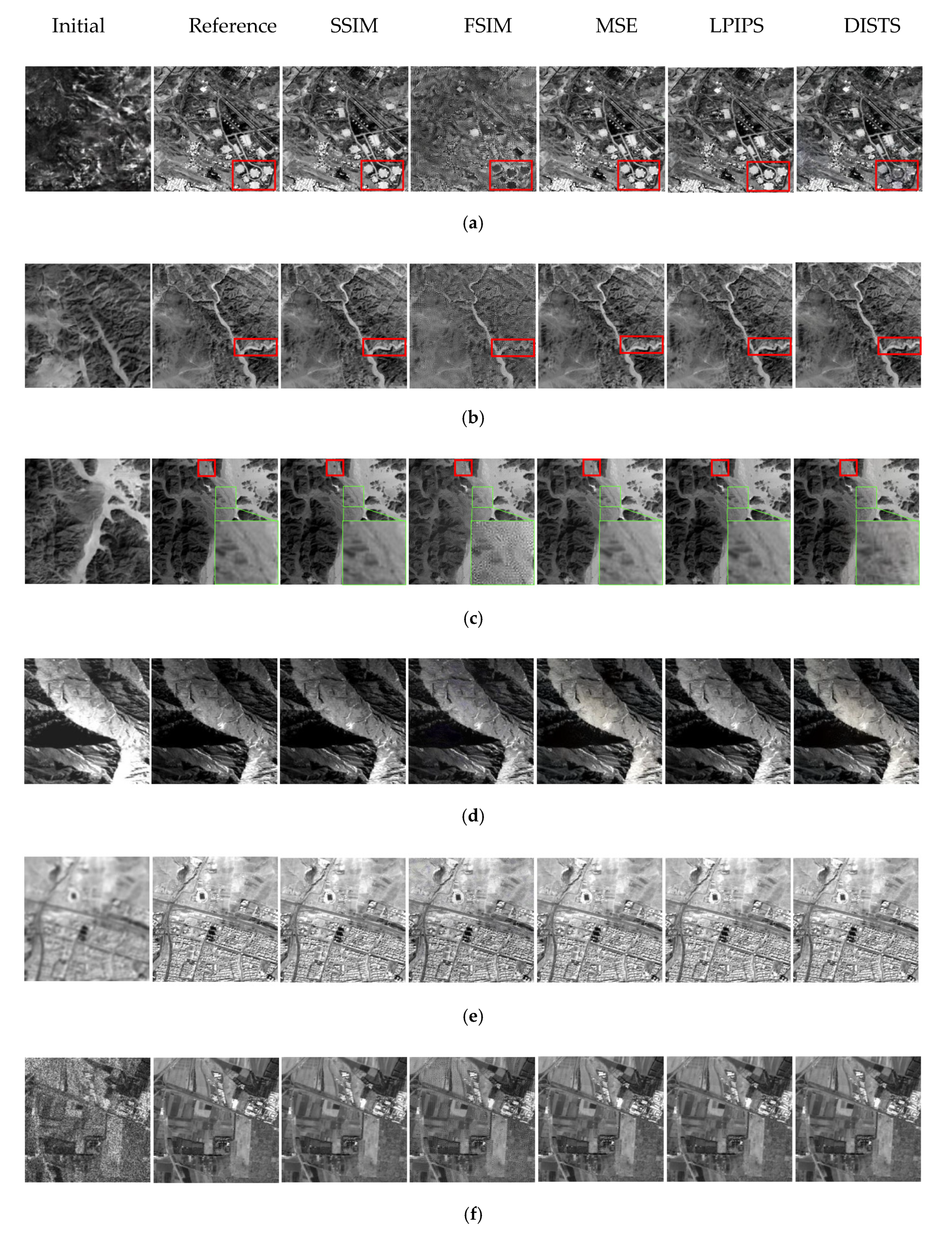
In order to find metrics suitable for evaluating the quality of the translation results, we carry out image restoration experiments in this section. In Figure 6, the first column shows the initial distorted images. The second column displays the reference images, with which the restored images on the right-hand columns are compared. Figure 6a–c show GAN distortions obtained by different image translation models respectively: pix2pix, CycleGAN and pix2pixHD. They differ from each other due to the network structure and generalization performance. Representative scenes are selected here, such as Industrial Area, River and Gorge. Figure 6d–f represent traditional distortion containing contrast shift, Gaussian blur and speckle noise. Mountain, Residential and Farmland are chosen in this case for experiments. The aim is to restore the distorted images to the reference images. The rectangles highlight the details of the restoration results, which can be used as a guidance for visual perception. We use five IQA methods, i.e., SSIM, FSIM, MSE, LPIPS and DISTS, as objective functions in the restoration algorithm. The results guide us to select suitable measurements to assess the translation performance.
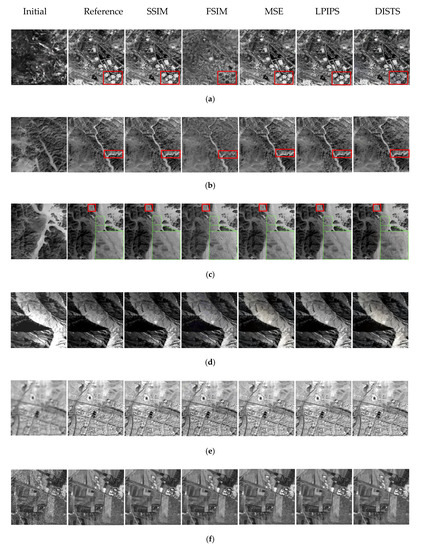
Figure 6.
Distorted Image Restoration results obtained by SSIM, feature similarity (FSIM), MSE, LPIPS and deep image structure and texture similarity (DISTS). (a) Industrial Area with pix2pix distortion, (b) River with CycleGAN distortion, (c) Gorge with pix2pixHD distortion, (d) Mountain with contrast shift, (e) Residential area with Gaussian blur, and (f) Farmland with speckle noise.
As shown in Figure 6, in the restoration of the GAN distorted images, point and line features are abundant in Figure 6a, which makes the restoration process more difficult. FSIM restores the general outline and structure, but lacks the details of textures, as well as low-level features. Meanwhile, DISTS has defects in contrast and saturation, shown in the red rectangle. Figure 6b exposes the insufficient capability of FSIM to restore tributaries. Because FSIM pays more attention to the extraction of high-level features, its performance is inconsistent with human perception. The same conclusion can be drawn from Figure 6c. The red rectangle marks a rock in the water, and the green rectangle marks a turbulent flow which is enlarged in the bottom right-hand corner of the image. After restoration, only SSIM, MSE and LPIPS recover the models. In Figure 6d–f, the texture of the mountains, the segmentation of the farmland, the orientation of the roads and the distribution of the residential areas have been generally restored from the traditional distorted images after 20,000 iterations. Metrics seem to be more sensitive to the traditional distortions and allow them to be more quickly restored. However, if the images are enlarged, spot noise will be found in FSIM. Point noise in images may increase the difficulty of feature extraction, leading to more failures.
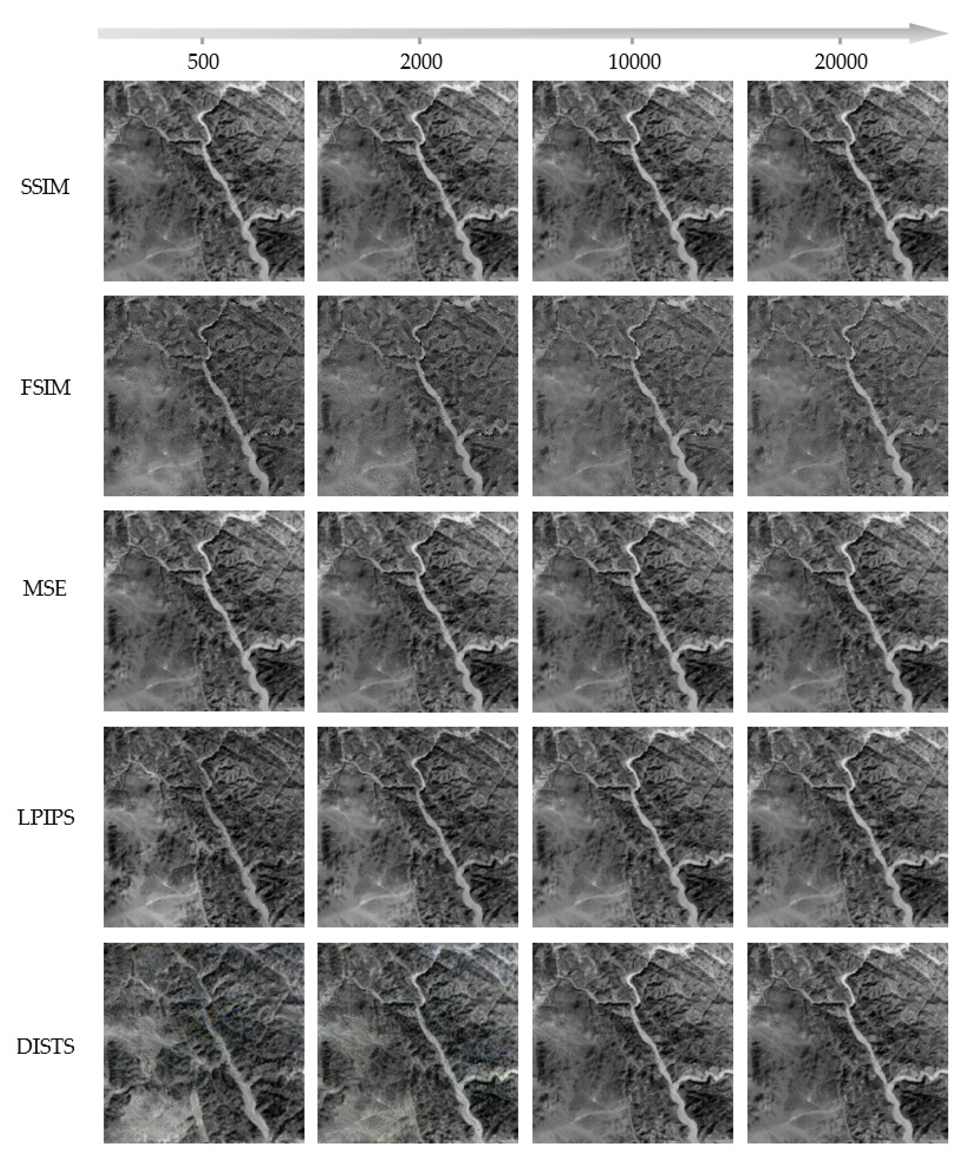
In order to show the process of image restoration, we take the River based on CycleGAN distortion as an example. We recover different models at 500, 2000, 10,000 and 20,000 iterations, and fit the “dist” convergence curve of the overall iterations. Figure 7 shows that after 500 iterations, SSIM, MSE and LPIPS have restored the general outline of the images, while FSIM and DISTS lack the details of the stream. DISTS makes a breakthrough in the process of 10,000 to 20,000 iterations and achieves satisfactory results in the end. Figure 8 displays that, among those metrics, SSIM and MSE converge faster than FSIM. In the CNN-based metrics, the convergence curve of LPIPS is faster and more stable than that of DISTS. Although MSE and LPIPS show several abnormal points, they quickly get back to normal. By contrast, DISTS has been fluctuating within 5000 iterations, which corresponds to the results shown in the bottom row of Figure 7.
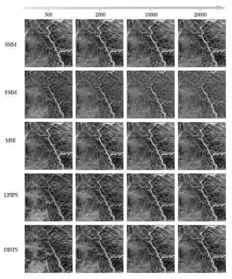
Figure 7.
Distorted Gorge recovery obtained by different models at 500, 2000, 10,000 and 20,000 iterations.

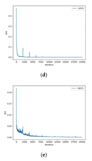
Figure 8.
Convergence curves of the whole iterations in Gorge restoration based on different IQA models. (a) SSIM; (b) FSIM; (c) MSE; (d) LPIPS; (e) DISTS.
We use a simple criterion to evaluate the effectiveness of the optimization results inspired by [16]. For a given visual task, image optimized via the IQA metric should achieve the best performance. When the recovered image based on metric
is evaluated via metric
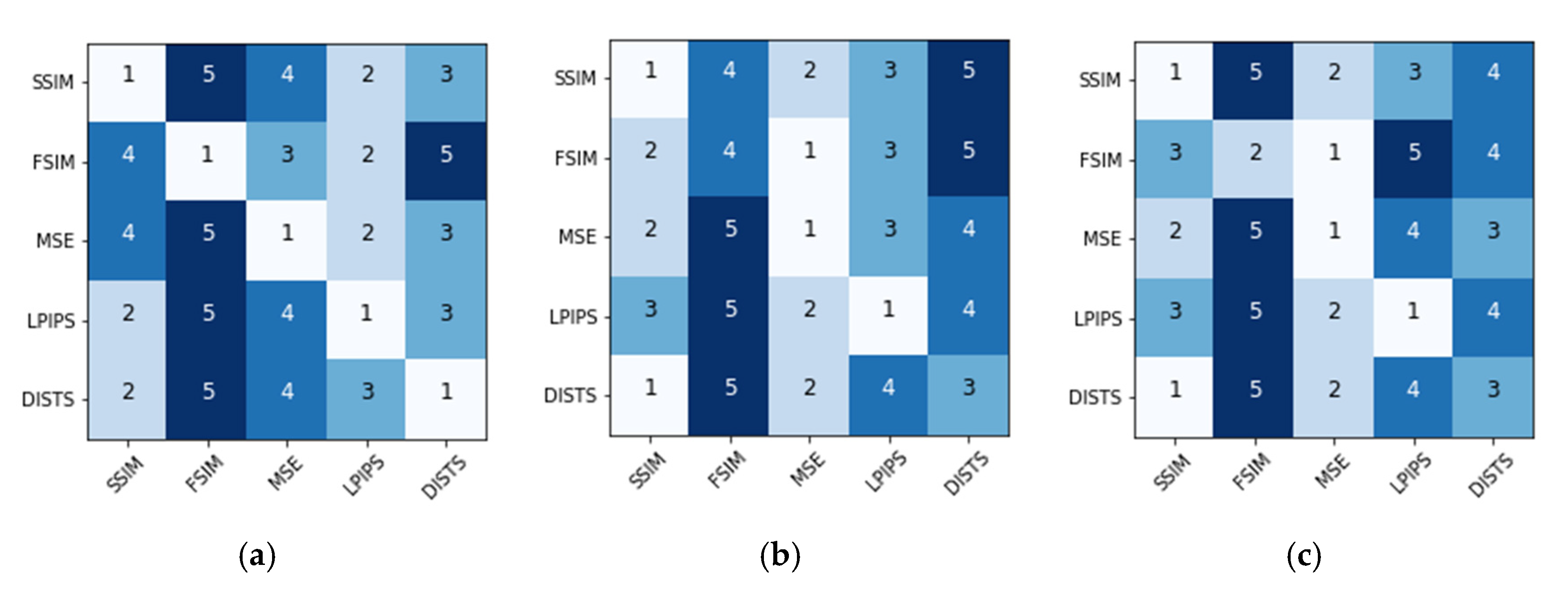
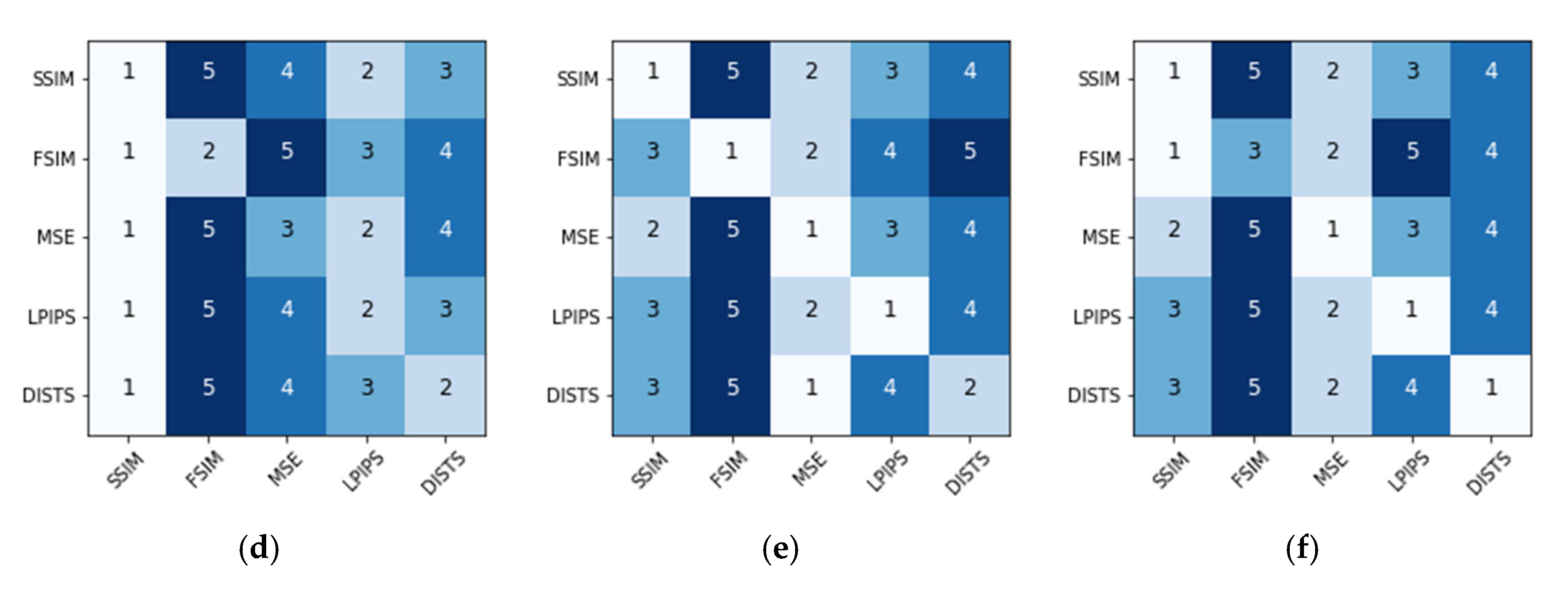
, it would obtain a score. Scores of all the metrics are ranked decreasingly. Higher ranking means better results using metric . It should be noted that unlike MSE, LPIPS and DISTS, larger values of SSIM and FSIM lead to higher ranking. Figure 9 represents the evaluation results of the recovered images optimized by five IQA models. Quantitative results of the ranking reference are shown in Appendix B Table A2. By inspecting the diagonal elements of the six matrices, we observe that 20 out of 30 models satisfy the criterion, verifying the rationality of using our training process. Among the remaining 10 models, 7 of them vote for SSIM and 3 for MSE, proving the robustness of SSIM and MSE in the restoration task. At the same time, 29 of 30 cases rank themselves on the top-3. In the list of the off-diagonal elements, FSIM and DISTS are ranked last 23 times and 4 times, respectively.

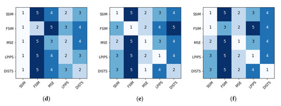
Figure 9.
Objective ranking of the restoration results optimized using IQA metrics. The horizontal axis represents the metrics used to train the image restoration network, and the vertical axis denotes the metrics used to evaluate the restoration performance. The number 1 to 5 indicate the rank order from the best to the worst. GAN and TRA mean GAN and Traditional distortions respectively. (a) GAN-Pix2pixHD. (b) GAN-Pix2pix; (c) GAN-CycleGAN; (d) TRA-contrast shift; (e) TRA-Gaussian blur. (f) TRA-speckle noise.
Meanwhile, in order to show the effect of IQA on the results of image restoration, the statistical analysis is illustrated in Table 3. We compute the differences between the initial and recovered images before and after performing IQA in our image restoration task. The first column represents different measurements. The second column contains the results before and after we have performed IQA involved in the right columns. As shown in Equation (14), the least-square method is performed if IQA is not used. Since diverse distortions are contained in the restoration task, we average the results obtained by the same method. Statistics show that IQA models especially SSIM, MSE and LPIPS play an important role in the process of restoration.

Table 3.
Statistical analysis on the effect of IQA on the results of image restoration. Unlike SSIM and FSIM, smaller values mean better results in MSE, LPIPS and DISTS.
Thus, we conclude that the objective IQA models can generally restore the distorted remote-sensing images to the reference ones, showing their appropriate feature recognition and availability for the stylization tasks. Furthermore, compared with FSIM and DISTS, SSIM, MSE and LPIPS show superior abilities, so we select SSIM, MSE and LPIPS to evaluate the translation results.
4.5. Objective Evaluation of Translation Results
We use SSIM, MSE and LPIPS to evaluate the images of multiple scenes obtained by the translation models. Because peak signal-to-noise ratio (PSNR) is closely related to MSE, as shown in Equation (16), its evaluation results are presented together with MSE. In order to make the assessment more comprehensive, we choose two baselines VGG [26] and SqueezeNet [27] to calculate LPIPS.
where denotes the maximum value of the image pixel color. It is 255 when the sample point is 8 bits. MSE represents the mean square error between the images.
It can be seen from Table 4 that FGGAN and pix2pixHD perform better than CycleGAN and pix2pix. Meanwhile, evaluations of all the metrics are consistent with each other, which shows that different metrics do not have conflicts, proving their availability for evaluation of image translation quality.

Table 4.
Objective evaluation of the images generated by the translation models. LPIPS adopts the linear structure. Bold in the table represents the best result using the metrics.
Multiple scenes are distinguished according to different features, such as line features in the farmland and roads, obvious folds on the mountains, point features in the residential areas, and so on. We try to search for the features for each individual model to extract. Ticks in Table 5 represent two of the five scenes with higher scores evaluated using the metrics shown before. In other words, the most suitable scenes for each model to translate are sought in this way. Because of the close relationship between PSNR and MSE, we combine them. Meanwhile, we unify the outcomes of different baselines in LPIPS. In this manner, a total of three standards are used to find the best features. It can be seen from the table that the top two in pix2pix are Forest and Gorge, and in CycleGAN they are Forest and River. Pix2pixHD is better at interpreting Farmland and River, and FGGAN is good at extracting Farmland and Forest. Residential translation is a difficult problem universally acknowledged by all the models.

Table 5.
Exploration of finding the most suitable scenes for each translation model.
4.6. Impact on Feature Extraction
In order to explore the effect of image translation on image feature extraction, a scene classification experiment is conducted. Results show the features of the generated images and reflect their benefits in applications such as regional planning and scene detection. Results can also be fed back to GANs in future studies for better translation performance.
We choose four classical feature extraction networks for image classification experiments: 18-layer ResNet, Inception, SqueezeNet and 19-layer VGG. Since CNN is good at calculating and extracting features that are used as the input of classifiers, we assess the performance of feature extraction and implement image classification by deploying full connection (FC) and softmax layers to classify the features extracted by CNNs, as shown in Figure 10. Models were pretrained on ImageNet. Images were divided into five categories which are the same as the translation part. Training models of the real optical images were used to examine the generated results.
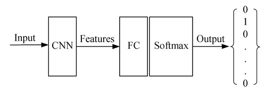
Figure 10.
Relationships between feature extraction and image classification. Convolutional neural networks (CNN) variants include 18-layer ResNet, Inception, SqueezeNet and 19-layer visual geometry group network(VGG).
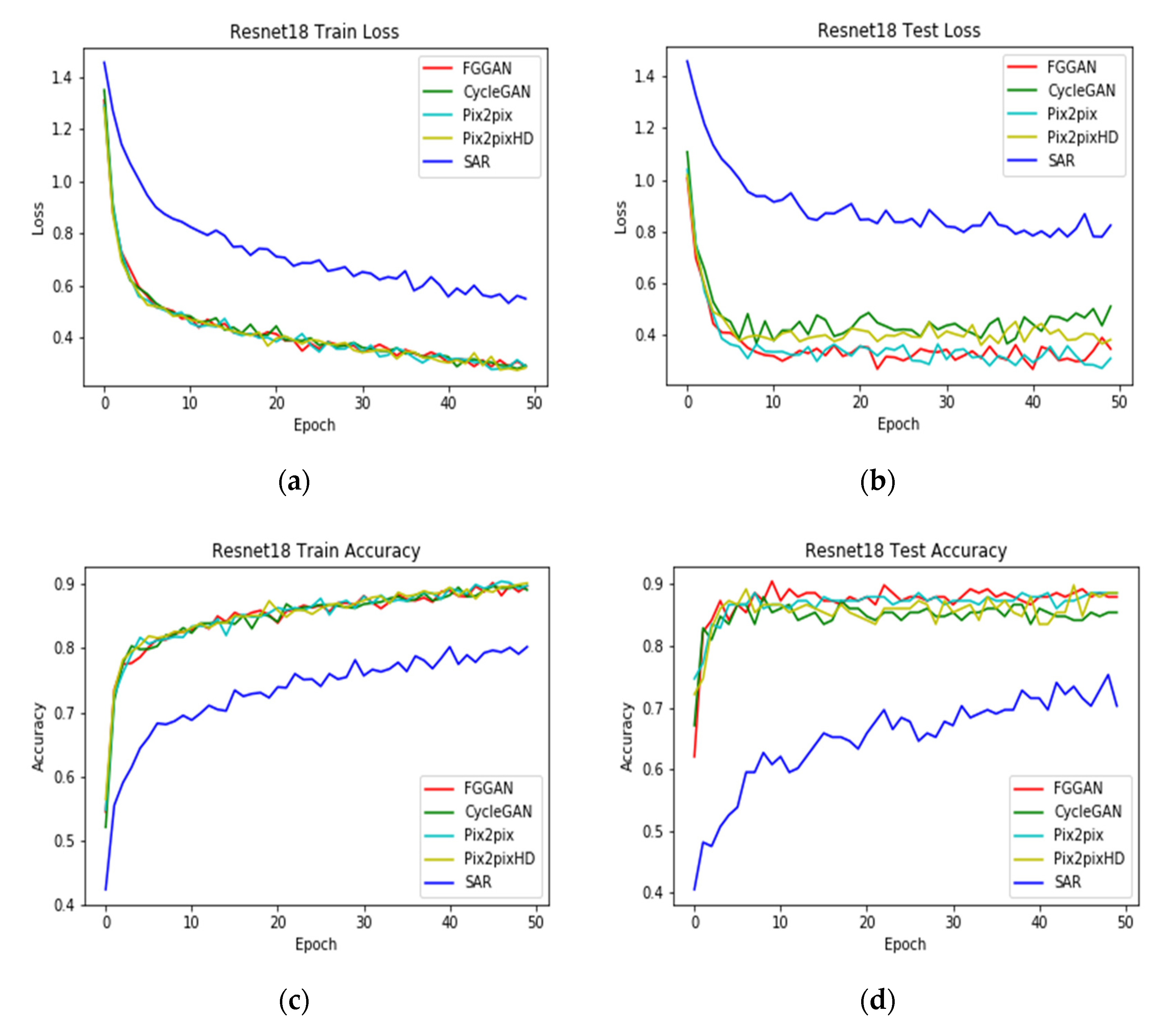
According to the loss function and accuracy curves shown in Figure 11 and top-1 accuracy illustrated in Table 6, the generated images are better than the original SAR images in multiple scenes for feature extraction. Training curves show that the convergence speed and accuracy of the real optical images are faster and higher, respectively, than those of the SAR images. Testing curves illustrate that the performance of the near-optical remote-sensing images is also better than that of the SAR images. It is specifically shown in Table 6 that the top-1 accuracy of classification for the generated images is as high as 90%, while that of the SAR images only reaches 75%. Thus, the capabilities of feature description and extraction of images are improved by image translation, leading to a wide application space. Furthermore, through the comparison of different translation models, inferences consistent with objective evaluation can be drawn: higher scores in the process of objective evaluation correspond to higher accuracy achieved in the scene classification.
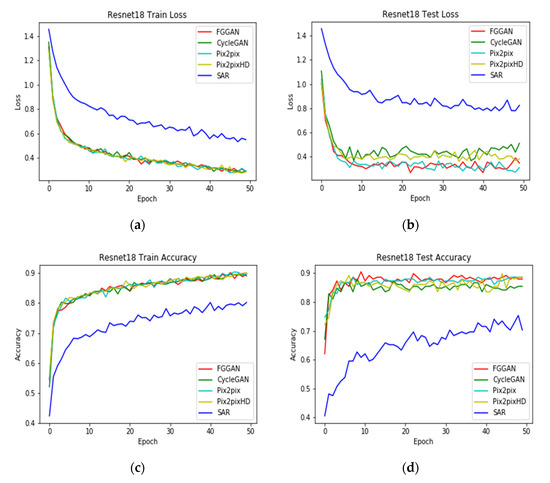
Figure 11.
Loss function and accuracy curves of classification experiments using 18-layer ResNet. (a) Loss function curve of the training sets. (b) Loss function curve of the test sets. (c) Accuracy curve of the training sets. (d) Accuracy curve of the test sets.

Table 6.
Top-1 accuracy of the models used in image classification experiments. Bold refers to the best classification result.
The accuracy of image classification before and after we have performed the IQA in our image restoration task is also computed and shown in Table 7. Note that, the results in the second row refer to the distances between the initial and recovered images, using the least-square method in the process of restoration. The results optimized by different IQA methods are shown in other rows. Table 7 shows that the accuracy is greatly improved after we have used IQA methods especially SSIM, MSE and LPIPS. Thus, IQA plays a key role in the process of restoration, which is consistent with the conclusion reached in Section 4.4.

Table 7.
Top-1 accuracy of image classification before and after performing the IQA in the image restoration task. Abbreviations w/o and w/ represent without and with, respectively. Bold refers to the top-3 classification result.
5. Conclusions and Outlook
In this paper, several image-to-image translation models were adopted as baselines to transform images from SAR images to optical images. The generated results were systematically evaluated based on the feedback from human visual inspection and objective IQA methods. The results offered a basis to analyze different remote-sensing image translation models. Scientific guidance for the optimization of the models and algorithms was also provided in this paper. Because the goal of translation is to achieve SAR image interpretation in the absence of reference optical images, the proposed IQA methods can be applied to different translation models for improving the results in the next step.
There are still some limitations in the proposed method. The current work does not analyze the influence of SAR polarizations (i.e., single to quad polarizations) and the effects of these methodologies on other collection modes outside of IW. In addition, IQA methods which are information theoretic and fusion-based are not mentioned here, because they have been proved to be inferior in previous studies [16]. However, our work can still be used as an exploratory method in the evaluation and optimization of SAR-to-optical image translation.
Future work will focus on the data augmentation, architecture designs and algorithm optimization for system performance improvement.
Author Contributions
Conceptualization, J.Z. (Jiexin Zhang) and J.J.Z. (Jianjiang Zhou); methodology, J.J.Z. and M.L.; software, J.Z. (Jiexin Zhang) and T.Y.; validation, J.Z. (Jiexin Zhang), J.J.Z. (Jianjiang Zhou) and M.L.; formal analysis, M.L. and H.Z.; investigation, J.Z. (Jiexin Zhang); data curation, M.L. and T.Y.; writing—original draft preparation, J.Z. (Jiexin Zhang) and T.Y.; writing—review and editing, J.J.Z. (Jianjiang Zhou), M.L. and H.Z.; visualization, J.Z. (Jiexin Zhang), J.J.Z. (Jianjiang Zhou) and H.Z.; supervision, H.Z. All authors have read and agreed to the published version of the manuscript.
Funding
This research received no external funding.
Acknowledgments
This research is supported by the National Youth Science Foundation of China under (Grant No. 61501228) and the Key Laboratory of Radar Imaging and Microwave Photonics (Nanjing Univ. Aeronaut. Astronaut.), Ministry of Education, China.
Conflicts of Interest
The authors declare no conflict of interest.
Appendix A. Investigations on Remote-Sensing Datasets
In this paper, images were divided into five categories: Farmland, Forest, Gorge, River and Residential. The classification depended on our investigations of a large number of remote-sensing datasets. Details of the investigation are shown here.
- University of California (UC) Merced LandUse Datasets [34], contain 21 scene classes and 100 samples of size 256 × 256 in each class.
- Northwestern Polytechnical University—Remote Sensing Image Scene Classification (NWPU-RESISC)45 Dataset [35], is a publicly available benchmark for Remote Sensing Image Scene Classification (RESISC) created by NorthWestern Polytechnical University (NWPU) and contains 45 categories of scenarios.
- Aerial Image Dataset (AID) [36], has 30 different scene classes and about 200 to 400 samples of size 600 × 600 in each class.
- Gaofen Image Dataset (GID) [37], contains 150 high-quality GaoFen-2 (GF-2) images of more than 60 different cities in China. These images cover more than 50,000 square kilometers of geographic area.
- A Large-scale Dataset for Object DeTection in Aerial Images (DOTA)-v1.0 [38], has 15 categories of different scenes. The size of each image ranges from 800 × 800 to 4000 × 4000.
- DOTA-v1.5 Dataset [38], is an updated version of DOTA-v1.0 and contains 16 different scene classes.
- A Large-scale Dataset for Instance Segmentation in Aerial Images (iSAID) [39], comes with 655,451 object instances for 15 categories across 2806 high-resolution images.
- Wuhan University–Remote Sensing (WHU-RS)19 Dataset [40], has 19 different scene classes and 50 samples of size 600 × 600 in each class.
- Scene Image dataset designed by RS_IDEA Group in Wuhan University (SIRI-WHU) [41], has 12 different scene classes and 200 samples of size 200 × 200 in each class.
- Remote Sensing Classification (RSC)11 Dataset [42], has 11 different scene classes and more than 100 samples of size 512 × 512 in each class.
According to the classification of the above 10 remote-sensing image datasets, the scenes that have occurred more than 5 times are listed below. Such an investigation provides strong evidence for the scene classification of remote sensing images in our work. Firstly, because the translation from SAR images to optical images is a difficult task, the scenes with higher differences are discussed here. Those with single structures and texture were excluded, such as Grass and Beach. Secondly, considering the scale limitation of SAR images, we excluded small-scale targets such as Airplane, Storage tanks, Baseball court and Ground track field, which also avoided generating more high-frequency noise. Finally, considering the research object of Earth observation and scene monitoring, we chose Forest, River, Lake, Gorge, Farmland, Residential and Industrial to discuss. Among the scenes, the difference between gorge and lake surrounded by natural vegetation in the SEN1-2 dataset was not clear, so we incorporated Lake into the category of Gorge in this work. Moreover, due to the complexity of man-made structures, Residential and Industrial areas were indistinguishable in most cases. We merged them into the Residential category.

Table A1.
Scenes mentioned more than 5 times in the investigations on remote sensing datasets. The bold cases were analyzed in the experimental section.
Table A1.
Scenes mentioned more than 5 times in the investigations on remote sensing datasets. The bold cases were analyzed in the experimental section.
| Category | Scene | Number of Times |
|---|---|---|
| Natural | Grass | 8 |
| Forest | 7 | |
| River | 6 | |
| Lake1 | 6 | |
| Farmland | 6 | |
| Beach | 5 | |
| Artificial | Harbor | 8 |
| Residential | 7 | |
| Airplane | 6 | |
| Storage tank | 6 | |
| Baseball court | 5 | |
| Industrial | 5 | |
| Ground track field | 5 |
1 Lake is incorporated into the category of Gorge in this work, since the difference between gorge and lake surrounded by natural vegetation in the SEN1-2 dataset is not clear.
Appendix B. Supplementary Experimental Results
This section is a supplement to the experimental results shown in the main body. In the image translation experiment, some images involved in the transition regions could not be accurately classified. Thus, more translation results of various areas are given in Figure A1 to help support the conclusion drawn in the main body of the text. Multiple scenes were included for the mixed area of Farmland and Residential (the second row), the boundary between the sunny side and nightside of mountain (the third row), and so on.
In the image restoration experiment, we used a simple criterion to assess the effectiveness of the optimization results and rank the scores of the metrics from high to low. However, the rankings only showed relative competitiveness of the metrics. The scores under the evaluation of each other were not quantitatively reflected. Thus, specific values which guide the ranking of the evaluation metrics are displayed in Table A2 to supplement the explanation of the experimental details.
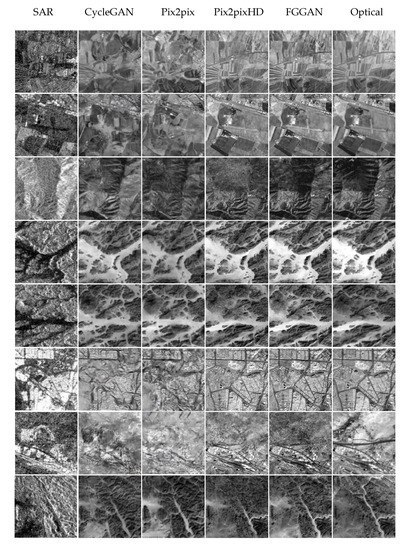
Figure A1.
More detailed results of SAR-to-optical image translation.
Figure A1.
More detailed results of SAR-to-optical image translation.
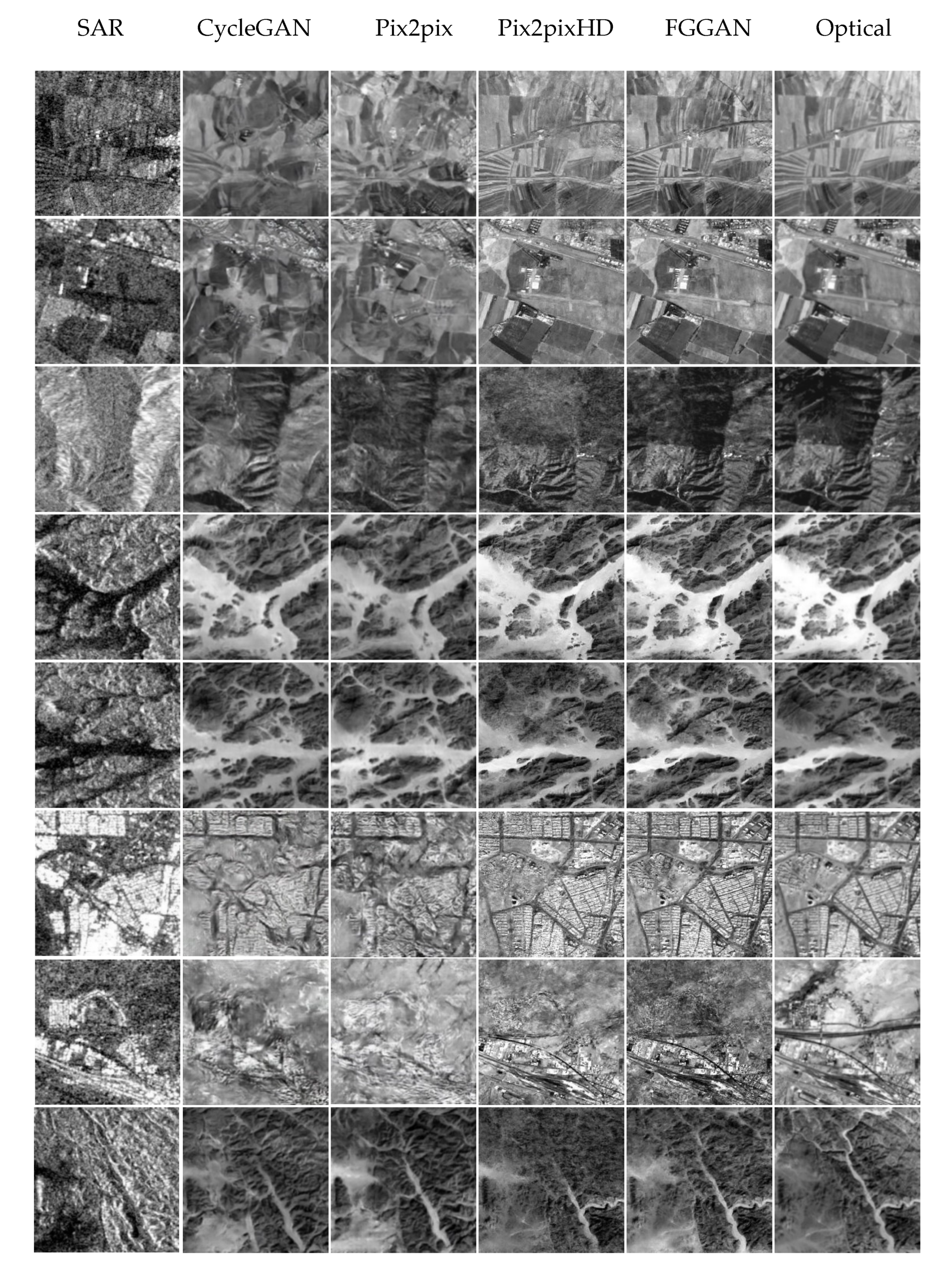

Table A2.
Quantitative data for guiding the ranking of the evaluation metrics. Unlike SSIM and FSIM, smaller values mean better results in MSE, LPIPS and DISTS. GAN and TRA in the header mean GAN distortion and Traditional distortion, respectively.
Table A2.
Quantitative data for guiding the ranking of the evaluation metrics. Unlike SSIM and FSIM, smaller values mean better results in MSE, LPIPS and DISTS. GAN and TRA in the header mean GAN distortion and Traditional distortion, respectively.
| Evaluation | Method | GAN—Pix2pixHD | GAN—Pix2pix | GAN—CycleGAN | TRA—Contrast Shift | TRA—Gaussian Blur | TRA—Speckle Noise |
|---|---|---|---|---|---|---|---|
| SSIM | SSIM | 0.9999 | 1.0000 | 1.0000 | 1.0000 | 1.0000 | 1.0000 |
| FSIM | 0.7245 | 0.9428 | 0.2370 | 0.7347 | 0.7123 | 0.4209 | |
| MSE | 0.9588 | 1.0000 | 1.0000 | 0.8626 | 1.0000 | 0.9999 | |
| LPIPS | 0.9997 | 0.9957 | 0.9985 | 0.9896 | 0.9994 | 0.9984 | |
| DISTS | 0.9917 | 0.9404 | 0.9805 | 0.8732 | 0.9947 | 0.9276 | |
| FSIM | SSIM | 0.9944 | 0.9999 | 0.9994 | 0.9999 | 0.9997 | 1.0000 |
| FSIM | 0.9999 | 0.9616 | 0.9999 | 0.9964 | 0.9999 | 0.9995 | |
| MSE | 0.9981 | 1.0000 | 1.0000 | 0.9575 | 0.9999 | 1.0000 | |
| LPIPS | 0.9998 | 0.9985 | 0.9576 | 0.9869 | 0.9970 | 0.9571 | |
| DISTS | 0.9840 | 0.9585 | 0.9884 | 0.9597 | 0.9851 | 0.9614 | |
| MSE | SSIM | 0.0022 | 0.0000 | 0.0000 | 0.0000 | 0.0000 | 0.0000 |
| FSIM | 0.0109 | 0.0832 | 0.0255 | 0.0046 | 0.0115 | 0.0025 | |
| MSE | 0.0000 | 0.0000 | 0.0000 | 0.0033 | 0.0000 | 0.0000 | |
| LPIPS | 0.0000 | 0.0011 | 0.0003 | 0.0018 | 0.0000 | 0.0001 | |
| DISTS | 0.0007 | 0.0039 | 0.0002 | 0.0045 | 0.0000 | 0.0002 | |
| LPIPS | SSIM | 0.0002 | 0.0023 | 0.0010 | 0.0000 | 0.0004 | 0.0006 |
| FSIM | 0.2923 | 0.5398 | 0.6180 | 0.1801 | 0.2371 | 0.2447 | |
| MSE | 0.0092 | 0.0001 | 0.0000 | 0.0501 | 0.0000 | 0.0002 | |
| LPIPS | 0.0000 | 0.0000 | 0.0000 | 0.0048 | 0.0000 | 0.0001 | |
| DISTS | 0.0053 | 0.0345 | 0.0127 | 0.0459 | 0.0026 | 0.0352 | |
| DISTS | SSIM | 0.0031 | 0.0000 | 0.0000 | 0.0000 | 0.0013 | 0.0037 |
| FSIM | 0.2361 | 0.5437 | 0.4756 | 0.1877 | 0.2514 | 0.2447 | |
| MSE | 0.0299 | 0.0002 | 0.0000 | 0.1033 | 0.0001 | 0.0016 | |
| LPIPS | 0.0198 | 0.0815 | 0.0324 | 0.0935 | 0.0101 | 0.0504 | |
| DISTS | 0.0003 | 0.0250 | 0.0153 | 0.0409 | 0.0002 | 0.0002 |
References
- Fuentes Reyes, M.; Auer, S.; Merkle, N.; Henry, C.; Schmitt, M. Sar-to-optical image translation based on conditional generative adversarial networks—Optimization, opportunities and limits. Remote Sens. 2019, 11, 2067. [Google Scholar] [CrossRef]
- Argenti, F.; Lapini, A.; Bianchi, T.; Alparone, L. A tutorial on speckle reduction in synthetic aperture radar images. IEEE Geosci. Remote Sens. Mag. 2013, 1, 6–35. [Google Scholar] [CrossRef]
- Fu, S.; Xu, F.; Jin, Y.Q. Translating SAR to optical images for assisted interpretation. arXiv 2019, arXiv:1901.03749. [Google Scholar]
- Toriya, H.; Dewan, A.; Kitahara, I. SAR2OPT: Image alignment between multi-modal images using generative adversarial networks. In Proceedings of the IGARSS 2019-2019 IEEE International Geoscience and Remote Sensing Symposium, Yokohama, Japan, 28 July–2 August 2019; pp. 923–926. [Google Scholar]
- Enomoto, K.; Sakurada, K.; Wang, W.; Kawaguchi, N.; Matsuoka, M.; Nakamura, R. Image translation between SAR and optical imagery with generative adversarial nets. In Proceedings of the IGARSS 2018-2018 IEEE International Geoscience and Remote Sensing Symposium, Valencia, Spain, 22–27 July 2018; pp. 1752–1755. [Google Scholar]
- Ley, A.; Dhondt, O.; Valade, S.; Haensch, R.; Hellwich, O. Exploiting GAN-based SAR to optical image transcoding for improved classification via deep learning. In Proceedings of the EUSAR 2018; 12th European Conference on Synthetic Aperture Radar, Aachen, Germany, 4–7 June 2018; pp. 1–6. [Google Scholar]
- Isola, P.; Zhu, J.Y.; Zhou, T.; Efros, A.A. Image-to-image translation with conditional adversarial networks. In Proceedings of the IEEE Conference on Computer Vision and Pattern Recognition 2017, Honolulu, HI, USA, 21–26 July 2017; pp. 1125–1134. [Google Scholar]
- Zhu, J.Y.; Park, T.; Isola, P.; Efros, A.A. Unpaired image-to-image translation using cycle-consistent adversarial networks. In Proceedings of the IEEE International Conference on Computer Vision 2017, Venice, Italy, 22–29 October 2017; pp. 2223–2232. [Google Scholar]
- Wang, T.C.; Liu, M.Y.; Zhu, J.Y.; Tao, A.; Kautz, J.; Catanzaro, B. High-resolution image synthesis and semantic manipulation with conditional gans. In Proceedings of the IEEE Conference on Computer Vision and Pattern Recognition 2018, Salt Lake City, UT, USA, 18–22 June 2018; pp. 8798–8807. [Google Scholar]
- Zhang, J.; Zhou, J.; Lu, X. Feature-Guided SAR-to-Optical Image Translation. IEEE Access 2020, 8, 70925–70937. [Google Scholar] [CrossRef]
- Wang, L.; Xu, X.; Yu, Y.; Yang, R.; Gui, R.; Xu, Z.; Pu, F. SAR-to-optical image translation using supervised cycle-consistent adversarial networks. IEEE Access 2019, 7, 129136–129149. [Google Scholar] [CrossRef]
- Wang, Z. Applications of objective image quality assessment methods [applications corner]. IEEE Signal Process. Mag. 2011, 28, 137–142. [Google Scholar] [CrossRef]
- Channappayya, S.S.; Bovik, A.C.; Caramanis, C.; Heath, R.W. SSIM-optimal linear image restoration. In Proceedings of the 2008 IEEE International Conference on Acoustics, Speech and Signal Processing, Las Vegas, NV, USA, 31 March–4 April 2008; pp. 765–768. [Google Scholar]
- Wang, S.; Rehman, A.; Wang, Z.; Ma, S.; Gao, W. SSIM-motivated rate-distortion optimization for video coding. IEEE Trans. Circuits Syst. Video Technol. 2011, 22, 516–529. [Google Scholar] [CrossRef]
- Snell, J.; Ridgeway, K.; Liao, R.; Roads, B.D.; Mozer, M.C.; Zemel, R.S. Learning to generate images with perceptual similarity metrics. In Proceedings of the 2017 IEEE International Conference on Image Processing (ICIP), Beijing, China, 17–20 September 2017; pp. 4277–4281. [Google Scholar]
- Ding, K.; Ma, K.; Wang, S.; Simoncelli, E.P. Comparison of Image Quality Models for Optimization of Image Processing Systems. arXiv 2020, arXiv:2005.01338. [Google Scholar]
- Shen, Z.; Huang, M.; Shi, J.; Xue, X.; Huang, T.S. Towards instance-level image-to-image translation. In Proceedings of the IEEE Conference on Computer Vision and Pattern Recognition 2019, Long Beach, CA, USA, 16–20 June 2019; pp. 3683–3692. [Google Scholar]
- Bishop, C.M. Pattern Recognition and Machine Learning; Springer: Berlin/Heidelberg, Germany, 2006. [Google Scholar]
- Wang, Z.; Bovik, A.C. Mean squared error: Love it or leave it? A new look at signal fidelity measures. IEEE Signal Process. Mag. 2009, 26, 98–117. [Google Scholar] [CrossRef]
- Wang, Z.; Bovik, A.C.; Sheikh, H.R.; Simoncelli, E.P. Image quality assessment: From error visibility to structural similarity. IEEE Trans. Image Process. 2004, 13, 600–612. [Google Scholar] [CrossRef] [PubMed]
- Zhang, L.; Zhang, L.; Mou, X.; Zhang, D. FSIM: A feature similarity index for image quality assessment. IEEE Trans. Image Process. 2011, 20, 2378–2386. [Google Scholar] [CrossRef] [PubMed]
- Ding, K.; Ma, K.; Wang, S.; Simoncelli, E.P. Image quality assessment: Unifying structure and texture similarity. arXiv 2020, arXiv:2004.07728. [Google Scholar]
- Osberger, W.; Bergmann, N.; Maeder, A. An automatic image quality assessment technique incorporating high level perceptual factors. In Proceedings of the IEEE International Conference on Image Processing 1998, Chicago, IL, USA, 4–7 October 1998; pp. 414–418. [Google Scholar]
- Markman, A.B.; Gentner, D. Nonintentional similarity processing. New Unconscious 2005, 2, 107–137. [Google Scholar]
- Zhang, R.; Isola, P.; Efros, A.A.; Shechtman, E.; Wang, O. The unreasonable effectiveness of deep features as a perceptual metric. In Proceedings of the IEEE Conference on Computer Vision and Pattern Recognition 2018, Salt Lake City, UT, USA, 18–22 June 2018; pp. 586–595. [Google Scholar]
- Simonyan, K.; Zisserman, A. Very deep convolutional networks for large-scale image recognition. arXiv 2014, arXiv:1409.1556. [Google Scholar]
- Iandola, F.N.; Han, S.; Moskewicz, M.W.; Ashraf, K.; Dally, W.J.; Keutzer, K. SqueezeNet: AlexNet-level accuracy with 50x fewer parameters and < 0.5 MB model size. arXiv 2016, arXiv:1602.07360. [Google Scholar]
- He, K.; Zhang, X.; Ren, S.; Sun, J. Deep residual learning for image recognition. In Proceedings of the IEEE Conference on Computer Vision and Pattern Recognition 2016, Las Vegas, NV, USA, 27–30 June 2016; pp. 770–778. [Google Scholar]
- Szegedy, C.; Liu, W.; Jia, Y.; Sermanet, P.; Reed, S.; Anguelov, D.; Erhan, D.; Vanhoucke, V.; Rabinovich, A. Going deeper with convolutions. In Proceedings of the IEEE Conference on Computer Vision and Pattern Recognition 2015, Boston, MA, USA, 8–12 June 2015; pp. 1–9. [Google Scholar]
- Krizhevsky, A.; Sutskever, I.; Hinton, G.E. Imagenet classification with deep convolutional neural networks. In Proceedings of the 25th International Conference on Neural Information Processing Systems, New York, NY, USA, 3–8 December 2012; pp. 1097–1105. [Google Scholar]
- Lim, B.; Son, S.; Kim, H.; Nah, S.; Mu Lee, K. Enhanced deep residual networks for single image super-resolution. In Proceedings of the IEEE Conference on Computer Vision and Pattern Recognition Workshops 2017, Honolulu, HI, USA, 21–26 July 2017; pp. 136–144. [Google Scholar]
- Schmitt, M.; Hughes, L.H.; Zhu, X.X. The SEN1-2 dataset for deep learning in SAR-optical data fusion. arXiv 2018, arXiv:1807.01569. [Google Scholar] [CrossRef]
- Zhang, R.; Isola, P.; Efros, A.A. Colorful image colorization. In Proceedings of the European Conference on Computer Vision 2016, Amsterdam, The Netherlands, 8–16 October 2016; pp. 649–666. [Google Scholar]
- UC Merced Land Use Dataset. Available online: http://weegee.vision.ucmerced.edu/datasets/landuse.html (accessed on 28 October 2010).
- Cheng, G.; Han, J.; Lu, X. Remote sensing image scene classification: Benchmark and state of the art. Proc. IEEE 2017, 105, 1865–1883. [Google Scholar] [CrossRef]
- Xia, G.S.; Hu, J.; Hu, F.; Shi, B.; Bai, X.; Zhong, Y.; Zhang, L. AID: A benchmark data set for performance evaluation of aerial scene classification. IEEE Trans. Geosci. Remote Sens. 2017, 55, 3965–3981. [Google Scholar] [CrossRef]
- Demir, I.; Koperski, K.; Lindenbaum, D.; Pang, G.; Huang, J.; Basu, S.; Hughes, F.; Tuia, D.; Raskar, R. A challenge to parse the earth through satellite images. arXiv 2018, arXiv:1805.06561. [Google Scholar]
- Xia, G.S.; Bai, X.; Ding, J.; Zhu, Z.; Belongie, S.; Luo, J.; Datcu, M.; Pelillo, M.; Zhang, L. DOTA: A large-scale dataset for object detection in aerial images. In Proceedings of the IEEE Conference on Computer Vision and Pattern Recognition 2018, Salt Lake City, UT, USA, 18–22 June 2018; pp. 3974–3983. [Google Scholar]
- Waqas Zamir, S.; Arora, A.; Gupta, A.; Khan, S.; Sun, G.; Shahbaz Khan, F.; Zhu, F.; Shao, L.; Xia, G.-S.; Bai, X. ISAID: A large-scale dataset for instance segmentation in aerial images. In Proceedings of the IEEE Conference on Computer Vision and Pattern Recognition Workshops 2019, Long Beach, CA, USA, 16–20 June 2019; pp. 28–37. [Google Scholar]
- Dai, D.; Yang, W. Satellite image classification via two-layer sparse coding with biased image representation. IEEE Geosci. Remote Sens. Lett. 2010, 8, 173–176. [Google Scholar] [CrossRef]
- Zhong, Y. Available online: http://www.lmars.whu.edu.cn/prof_web/zhongyanfei/e-code.html (accessed on 19 April 2016).
- RSC11Datasets. Available online: https://www.researchgate.net/publication/271647282_RS_C11_Database (accessed on 31 January 2015).
Publisher’s Note: MDPI stays neutral with regard to jurisdictional claims in published maps and institutional affiliations. |
© 2020 by the authors. Licensee MDPI, Basel, Switzerland. This article is an open access article distributed under the terms and conditions of the Creative Commons Attribution (CC BY) license (http://creativecommons.org/licenses/by/4.0/).


