Cross-Validation of Radio-Frequency-Interference Signature in Satellite Microwave Radiometer Observations over the Ocean


Abstract

1. Introduction
2. AMSR2 Data
3. RFI Detection Methods
3.1. GRDM Method
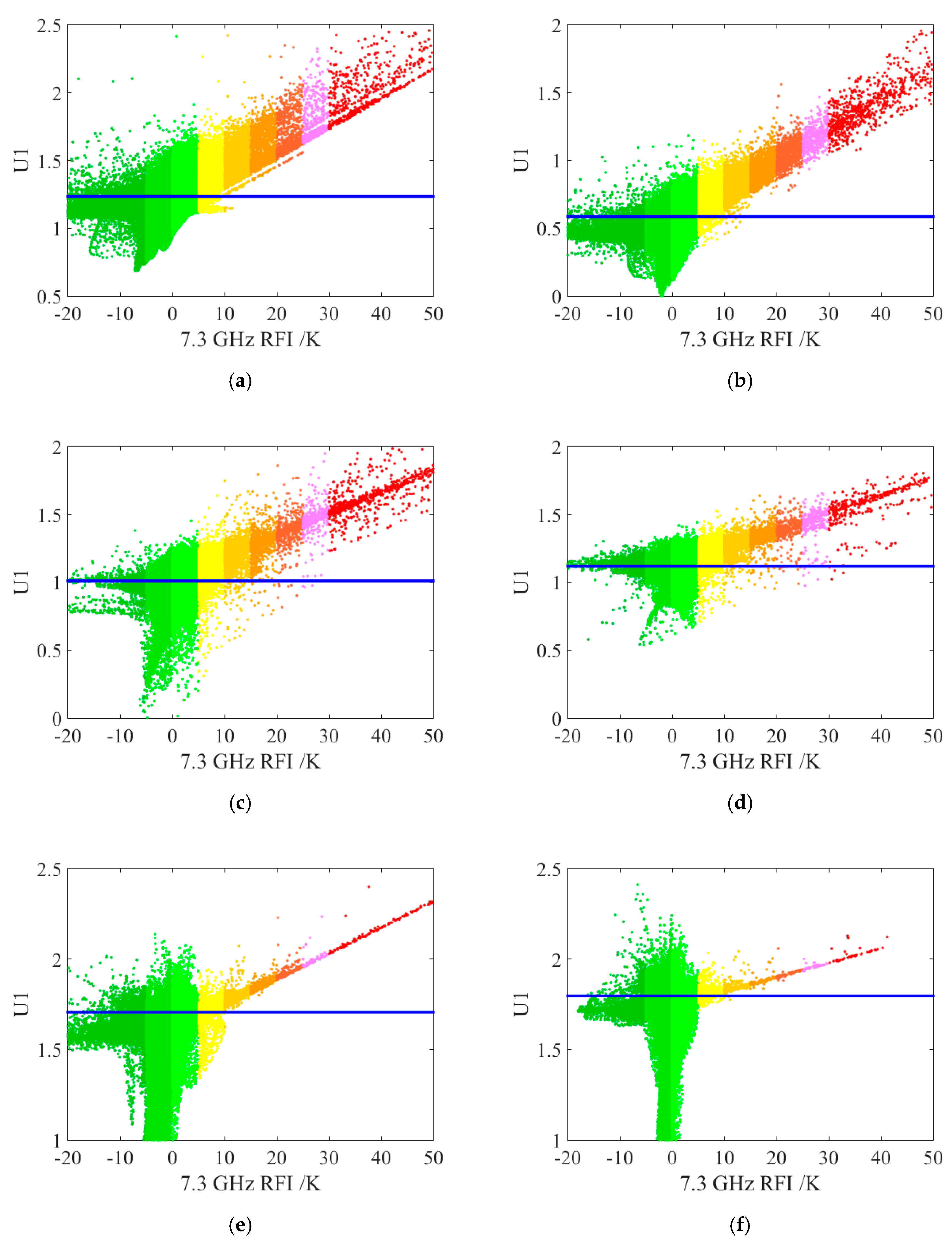
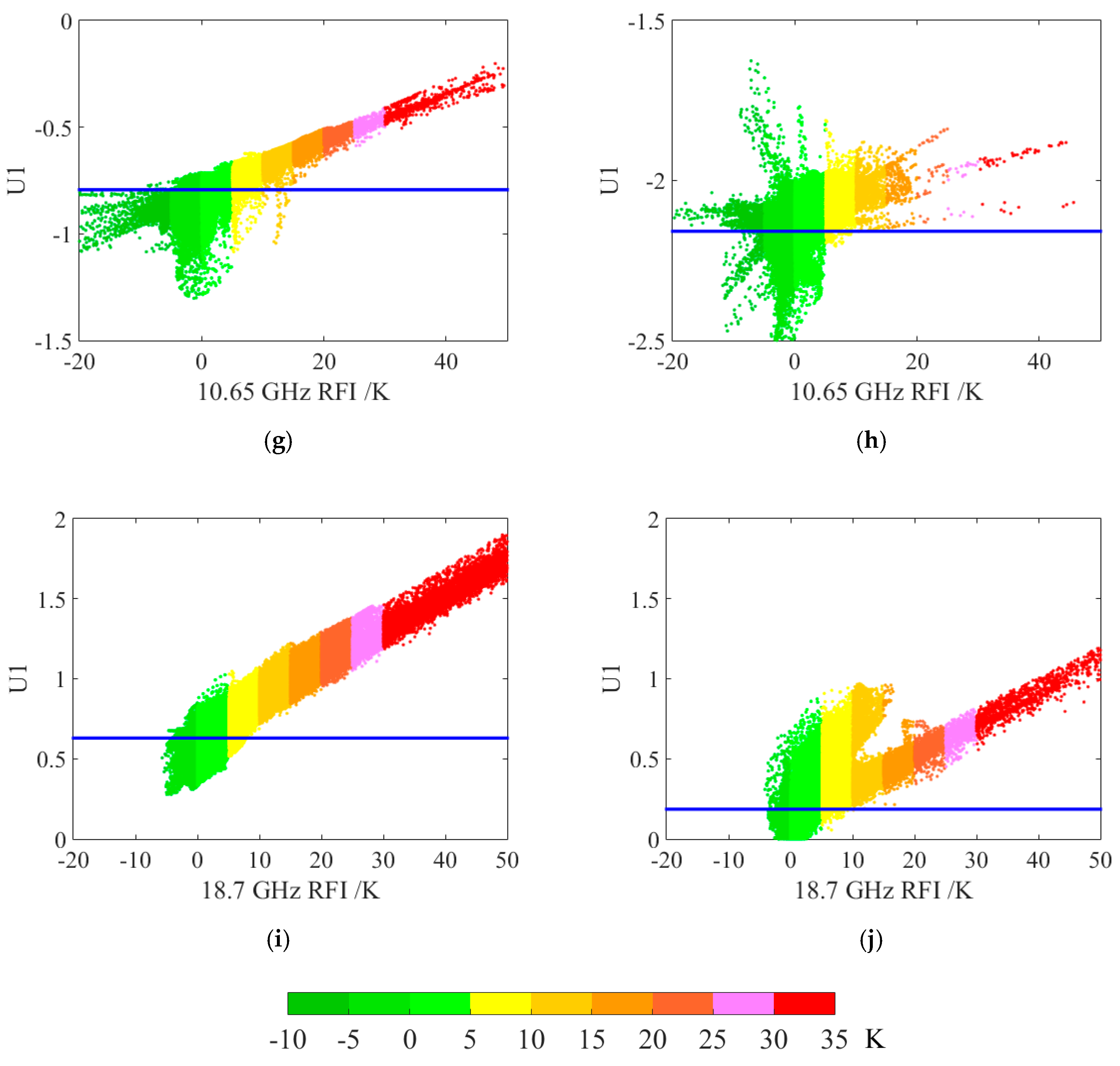
3.2. DPCA Method
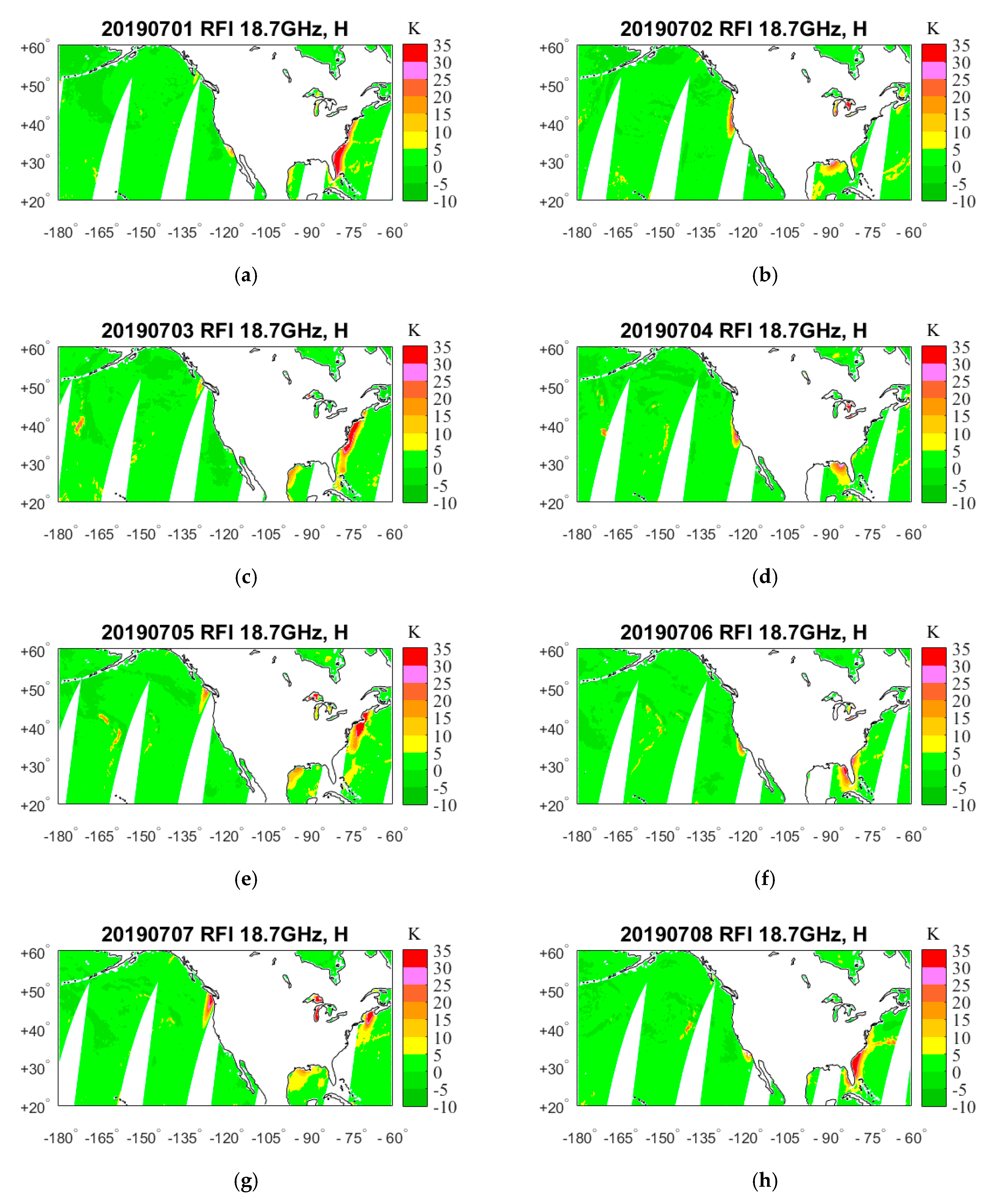
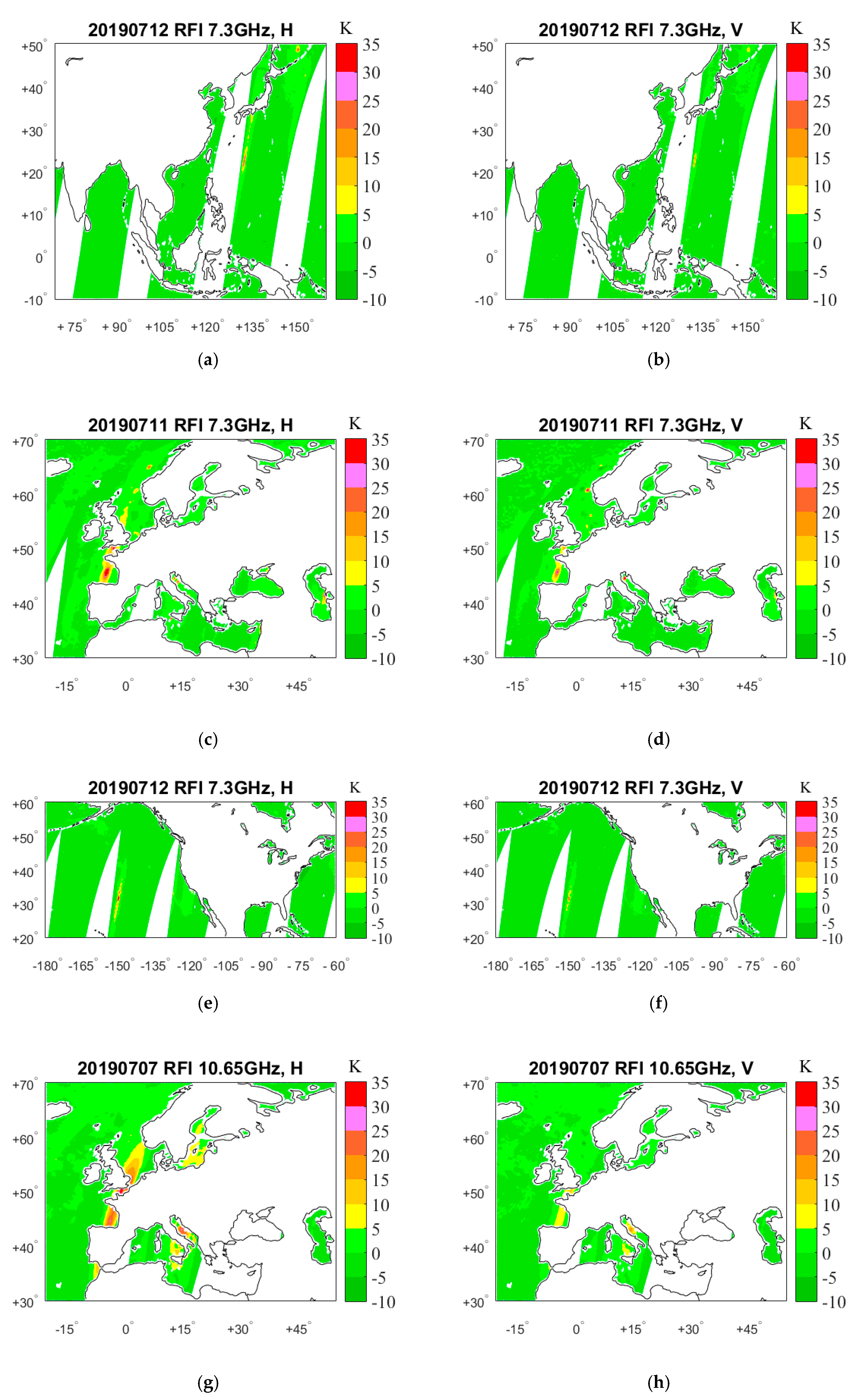
4. Results
4.1. RFI Detection by GRDM
4.2. RFI Detection by DPCA
5. RFI Source Analysis
6. Conclusions
Author Contributions
Funding
Acknowledgments
Conflicts of Interest
References
- Li, L.; Njoku, E.G.; Im, E.; Chang, P.S.; Germain, K.S. A preliminary survey of radio-frequency Interference over the U.S. in Aqua AMSR-E data. IEEE Trans. Geosci. Remote Sens. 2004, 42, 380–390. [Google Scholar] [CrossRef]
- Njoku, E.G.; Ashcroft, P.; Chan, T.K.; Li, L. Global survey and statistics of Radio-Frequency Interference in AMSR-E land observations. IEEE Trans. Geosci. Remote Sens. 2005, 43, 938–947. [Google Scholar] [CrossRef]
- Kidd, C. Radio frequency interference at passive microwave earth observation frequencies. Int. J. Remote Sens. 2006, 27, 3853–3865. [Google Scholar] [CrossRef]
- Yang, H.; Weng, F. Error sources in remote sensing of microwave land surface emissivity. IEEE Trans. Geosci. Remote Sens. 2011, 49, 3437–3442. [Google Scholar] [CrossRef]
- Wu, Y.; Weng, F. Applications of an AMSR-E RFI detection and correction algorithm in 1-DVAR over land. J. Meteorol. Res. 2014, 28, 645–655. [Google Scholar] [CrossRef]
- Zou, X.; Zhao, J.; Weng, F.; Qin, Z. Detection of radio-frequency interference signal over land from FY-3B Microwave Radiation Imager (MWRI). IEEE Trans. Geosci. Remote Sens. 2012, 40, 4994–5003. [Google Scholar] [CrossRef]
- Wu, Y.; Weng, F. Detection and correction of AMSR-E radio-frequency interference. Acta Meteorol. Sin. 2011, 25, 669–681. [Google Scholar] [CrossRef]
- Lacava, T.; Coviello, I.; Faruolo, M.; Mazzeo, G.; Pergola, N.; Tramutoli, V. A multitemporal investigation of AMSR-E C-band radio-frequency interference. IEEE Trans. Geosci. Remote Sens. 2013, 51, 2007–2015. [Google Scholar] [CrossRef]
- Wu, Y.; Qian, B.; Bao, Y.; Li, M.; Petropoulos, G.P.; Liu, X.; Li, L. Detection and analysis of c-band radio frequency interference in AMSR2 data over land. Remote Sens. 2019, 11, 1228. [Google Scholar] [CrossRef]
- Du, J.; Kimball, J.; Shi, J.; Jones, L.; Wu, S.; Sun, R.; Yang, H. Inter-calibration of satellite passive microwave land observations from AMSR-E and AMSR2 using overlapping FY3B-MWRI sensor measurements. Remote Sens. 2014, 6, 8594–8616. [Google Scholar] [CrossRef]
- Draper, D.W.; Newell, D.A.; Wentz, F.J.; Krimchansky, S. The Global Precipitation Measurement (GPM) Microwave Imager (GMI): Instrument overview and early on-orbit performance. IEEE J. Sel. Top. Appl. Earth Obs. Remote Sens. 2015, 8, 3452–3462. [Google Scholar] [CrossRef]
- Ellingson, S.W.; Johnson, J.T. A polarimetric survey of radio-frequency interference in C-and X-bands in the continental United States using WindSat radiometry. IEEE Trans. Geosci. Remote Sens. 2006, 44, 540–548. [Google Scholar] [CrossRef]
- Li, L.; Gaiser, P.W.; Bettenhausen, M.H.; Johnston, W. WindSat radio-frequency interference signature and its identification over land and ocean. IEEE Trans. Geosci. Remote Sens. 2006, 44, 530–539. [Google Scholar] [CrossRef]
- Zhao, J.; Zou, X.; Weng, F. WindSat radio-frequency interference signature and its identification over Green land and Antarctic. IEEE Trans. Geosci. Remote Sens. 2013, 51, 4830–4839. [Google Scholar] [CrossRef]
- Candy, B.; Saunders, R.W.; Ghent, D.; Bulgin, C.E. The impact of satellite-derived land surface temperatures on numerical weather prediction analyses and forecasts. J. Geophys. Res. Atmos. 2017, 122, 9783–9802. [Google Scholar] [CrossRef]
- Al-Yaari, A.; Dayau, S.; Chipeaux, C.; Aluome, C.; Kruszewski, A.; Loustau, D.; Wigneron, J.P. The AQUI soil moisture network for satellite microwave remote sensing validation in south-eastern France. Remote Sens. 2018, 10, 1839. [Google Scholar] [CrossRef]
- Du, J.; Kimball, J.; Reichle, R.; Jones, L.; Watts, J.; Kim, Y. Global satellite retrievals of the near-surface atmospheric vapor pressure deficit from AMSR-E and AMSR2. Remote Sens. 2018, 10, 1175. [Google Scholar] [CrossRef]
- Pavelin, E.G.; Candy, B. Assimilation of surface-sensitive infrared radiances over land: Estimation of land surface temperature and emissivity. Q. J. R. Meteorol. Soc. 2014, 140, 1198–1208. [Google Scholar] [CrossRef]
- Xie, Y.; Shi, J.; Lei, Y.; Li, Y. Modeling microwave emission from short vegetation-covered surfaces. Remote Sens. 2015, 7, 14099–14118. [Google Scholar] [CrossRef]
- Grenkov, S.A.; Kol’tsov, N.E. Spectral-selective radiometer unit with radio-interference protection, radiophys. Quantum Electron. 2015, 58, 520–528. [Google Scholar]
- Metelev, S.; Lvov, A. Estimation of the potential interference immunity of radio reception with spatial signal processing in multipath radio-communication channels. I. decameter range. Radiophys. Quantum Electron. 2016, 59, 329–340. [Google Scholar] [CrossRef]
- Martin, G.M.; Milton, S.F.; Senior, C.A.; Brooks, M.E.; Ineson, S. Analysis and reduction of systematic errors through a seamless approach to modeling weather and climate. J. Clim. 2010, 23, 5933–5957. [Google Scholar] [CrossRef]
- Berg, W.; Kroodsma, R.; Kummerow, C.; McKague, D. Fundamental climate data records of microwave brightness temperatures. Remote Sens. 2018, 10, 1306. [Google Scholar] [CrossRef]
- Draper, D.; Newell, D. An assessment of radio-frequency interference using the GPM Microwave Imager. In Proceedings of the 2015 IEEE International Geoscience and Remote Sensing Symposium (IGARSS), Milan, Italy, 26–31 July 2015. [Google Scholar]
- Adams, I.S.; Bettenhausen, M.H.; Gaiser, P.W.; Johnston, W. Identification of ocean-reflected radio-frequency interference using WindSat retrieval chi-square probability. IEEE Geosci. Remote Sens. Lett. 2010, 7, 406–410. [Google Scholar] [CrossRef]
- Zabolotskikh, E.V.; Mitnik, L.M.; Chapron, B. Radio-frequency interference identification over oceans for C- and X-Band AMSR2 channels. IEEE Geosci. Remote Sens. Lett. 2015, 12, 1705–1709. [Google Scholar] [CrossRef]
- Zou, X.; Tian, X.; Weng, F. Detection of television frequency interference with satellite microwave imager observations over oceans. J. Atmos. Ocean. Technol. 2014, 31, 2759–2776. [Google Scholar] [CrossRef]
- Tian, X.; Zou, X. An empirical model for television frequency interference correction of AMSR2 data over ocean near the U.S. and Europe. IEEE Trans. Geosci. Remote Sens. 2016, 54, 3856–3867. [Google Scholar] [CrossRef]
- Kachi, M.; Imaoka, K.; Fujii, H.; Shibata, A.; Kasahara, M.; Iida, Y.; Ito, N.; Nakagawa, K.; Shimoda, H. Status of GCOM-W1/AMSR2 development and science activities. In Sensors, Systems, and Next-Generation Satellites XII; International Society for Optics and Photonics: Bellingham, WA, USA, 2008. [Google Scholar] [CrossRef]
- Weng, F.; Yan, B.; Grody, N.C. A microwave land emissivity model. J. Geophys. Res. 2001, 106, 20115–20123. [Google Scholar] [CrossRef]
- Guan, L.; Zhang, S. Source analysis of spaceborne microwave radiometer interference over land. Front. Earth Sci. 2016, 10, 135–144. [Google Scholar] [CrossRef]
- Radio Spectrum Allocation. Available online: https://www.fcc.gov/engineering-technology/policy-and-rules-division/general/radio-spectrum-allocation (accessed on 10 May 2020).


| Coefficients | ΔTB [i] | |||||||
|---|---|---|---|---|---|---|---|---|
| ΔTB[1] (i = 1) | ΔTB[2] (i = 2) | ΔTB[3] (i = 3) | ΔTB[4] (i = 4) | ΔTB[5] (i = 5) | ΔTB[6] (i = 6) | ΔTB[7] (i = 7) | ΔTB[8] (i = 8) | |
| a0[i] | −3.0385 | −2.1317 | −7.5344 | −6.7285 | 3.1463 | −0.8659 | 6.9579 | 12.5611 |
| a1[i] | 1 | 0 | −0.0669 | 0.6068 | −0.1435 | 0.3977 | −0.0199 | 0.0062 |
| a2[i] | 0 | 1 | 0.8919 | 0.1550 | 0.3742 | −0.0710 | 0.0320 | 0.0322 |
| a3[i] | −0.0567 | 0.3474 | 1 | 0 | −0.0139 | 0.1441 | −0.0575 | −0.0266 |
| a4[i] | 0.8847 | 0.3084 | 0 | 1 | 0.2023 | 0.0106 | 0.1325 | 0.0613 |
| a5[i] | 0.2131 | 0.8865 | −0.0301 | 0.3797 | 1 | 0 | 0.0161 | 0.2564 |
| a6[i] | 0.0159 | −0.4384 | 0.1141 | −0.1579 | 0 | 1 | 0.3029 | −0.0003 |
| a7[i] | 0.3984 | 0.3082 | 0.0001 | 0.0000 | 0.1261 | 0.5499 | 1 | 0 |
| a8[i] | −0.1549 | −0.1295 | 0.1459 | 0.0677 | 0.9142 | 0.3147 | 0 | 1 |
| a9[i] | −0.9438 | −0.7650 | 0.1827 | 0.0795 | 0.4251 | 0.2049 | 0.3741 | 0.8907 |
| a10[i] | 0.4591 | 0.3895 | −0.1249 | −0.0474 | −0.5352 | −0.3133 | 0.1404 | −0.2832 |
| a11[i] | 0.4613 | 0.1383 | −0.1138 | −0.1184 | −0.6113 | −0.4222 | −0.3277 | −0.0305 |
| a12[i] | −0.2518 | −0.0727 | −0.0227 | 0.0136 | 0.0703 | 0.0585 | 0.5223 | 0.1948 |
| a13[i] | −0.0475 | 0.0668 | 0.0653 | 0.0691 | 0.1955 | 0.1380 | −0.0369 | −0.1535 |
| a14[i] | 0.0218 | −0.0347 | −0.0065 | −0.0154 | −0.0077 | −0.0058 | −0.1053 | 0.0055 |
| Numbers of Detected RFI Pixels | ||||||||||
|---|---|---|---|---|---|---|---|---|---|---|
| Date (July) | 7.3 GHz | 10.65 GHz | 18.7 GHz | |||||||
| Asia | Europe | USA | Europe | USA | ||||||
| H | V | H | V | H | V | H | V | H | V | |
| 1 | 1710 | 998 | 2191 | 990 | 32 | 22 | 10,307 | 1396 | 13,552 | 4220 |
| 2 | 1298 | 935 | 3196 | 840 | 1624 | 15 | 6779 | 1602 | 16,391 | 2654 |
| 3 | 3802 | 1466 | 2432 | 797 | 164 | 14 | 11,026 | 917 | 17,933 | 5282 |
| 4 | 3028 | 2012 | 4301 | 1068 | 2172 | 231 | 9846 | 1139 | 12,464 | 3009 |
| 5 | 1968 | 979 | 2349 | 923 | 54 | 25 | 11,065 | 3338 | 20,567 | 4796 |
| 6 | 1537 | 1288 | 3202 | 1020 | 553 | 48 | 9069 | 1723 | 11,734 | 3186 |
| 7 | 1574 | 1391 | 1987 | 884 | 1438 | 0 | 8101 | 1960 | 20,099 | 4100 |
| 8 | 2700 | 1258 | 2289 | 798 | 114 | 41 | 7793 | 1689 | 13,432 | 5183 |
| 9 | 1792 | 1476 | 2121 | 768 | 587 | 253 | 7270 | 1159 | 15,467 | 3049 |
| 10 | 1556 | 814 | 2175 | 1104 | 974 | 231 | 12,102 | 1318 | 16,075 | 6050 |
| 11 | 1339 | 1020 | 2655 | 1348 | 2176 | 465 | 8081 | 1487 | 13,472 | 3762 |
| 12 | 2478 | 1555 | 1080 | 473 | 2002 | 714 | 11,172 | 2518 | 21,415 | 5450 |
| 13 | 1169 | 1257 | 1914 | 592 | 526 | 92 | 9683 | 2219 | 14,263 | 4100 |
| 14 | 1622 | 1273 | 899 | 722 | 2180 | 662 | 9741 | 2426 | 18,790 | 4266 |
| 15 | 3062 | 1785 | 1496 | 657 | 122 | 19 | 8139 | 1257 | 11,077 | 3522 |
| 16 | 764 | 960 | 1615 | 709 | 281 | 80 | 7220 | 1919 | 16,783 | 4506 |
| 7.3 GHz | 10.65 GHz | 18.7 GHz | ||||||||
|---|---|---|---|---|---|---|---|---|---|---|
| Asia | Europe | USA | Europe | USA | ||||||
| H | V | H | V | H | V | H | V | H | V | |
| U1thres | 1.2336 | 0.5845 | 1.0098 | 1.1172 | 1.7063 | 1.7965 | −0.7933 | −2.1587 | 0.6293 | 0.1865 |
Publisher’s Note: MDPI stays neutral with regard to jurisdictional claims in published maps and institutional affiliations. |
© 2020 by the authors. Licensee MDPI, Basel, Switzerland. This article is an open access article distributed under the terms and conditions of the Creative Commons Attribution (CC BY) license (http://creativecommons.org/licenses/by/4.0/).
Share and Cite
Wu, Y.; Li, M.; Bao, Y.; Petropoulos, G.P. Cross-Validation of Radio-Frequency-Interference Signature in Satellite Microwave Radiometer Observations over the Ocean. Remote Sens. 2020, 12, 3433. https://doi.org/10.3390/rs12203433
Wu Y, Li M, Bao Y, Petropoulos GP. Cross-Validation of Radio-Frequency-Interference Signature in Satellite Microwave Radiometer Observations over the Ocean. Remote Sensing. 2020; 12(20):3433. https://doi.org/10.3390/rs12203433
Chicago/Turabian StyleWu, Ying, Meixin Li, Yansong Bao, and George P. Petropoulos. 2020. "Cross-Validation of Radio-Frequency-Interference Signature in Satellite Microwave Radiometer Observations over the Ocean" Remote Sensing 12, no. 20: 3433. https://doi.org/10.3390/rs12203433
APA StyleWu, Y., Li, M., Bao, Y., & Petropoulos, G. P. (2020). Cross-Validation of Radio-Frequency-Interference Signature in Satellite Microwave Radiometer Observations over the Ocean. Remote Sensing, 12(20), 3433. https://doi.org/10.3390/rs12203433