Article

Bathymetric Inversion and Uncertainty Estimation from Synthetic Surf-Zone Imagery with Machine Learning

1
Coastal and Hydraulics Laboratory, U.S. Army Engineer Research and Development Center, 1261 Duck Rd, Duck, NC 27949, USA
2
Department of Earth and Ocean Sciences, University of North Carolina-Wilmington, Wilmington, NC 28405, USA
3
Coastal and Hydraulics Laboratory, U.S. Army Engineer Research and Development Center, 3909 Halls Ferry Rd, Vicksburg, MS 39180, USA
4
Department of Civil and Environmental Engineering, University of Hawai’i at Mānoa, Honolulu, HI 96822, USA
*
Author to whom correspondence should be addressed.
Remote Sens. 2020, 12(20), 3364; https://doi.org/10.3390/rs12203364
Submission received: 24 August 2020 / Revised: 2 October 2020 / Accepted: 7 October 2020 / Published: 15 October 2020
(This article belongs to the Special Issue Computer Vision and Deep Learning for Remote Sensing Applications)

Abstract

:
Resolving surf-zone bathymetry from high-resolution imagery typically involves measuring wave speeds and performing a physics-based inversion process using linear wave theory, or data assimilation techniques which combine multiple remotely sensed parameters with numerical models. In this work, we explored what types of coastal imagery can be best utilized in a 2-dimensional fully convolutional neural network to directly estimate nearshore bathymetry from optical expressions of wave kinematics. Specifically, we explored utilizing time-averaged images (timex) of the surf-zone, which can be used as a proxy for wave dissipation, as well as including a single-frame image input, which has visible patterns of wave refraction and instantaneous expressions of wave breaking. Our results show both types of imagery can be used to estimate nearshore bathymetry. However, the single-frame imagery provides more complete information across the domain, decreasing the error over the test set by approximately 10% relative to using timex imagery alone. A network incorporating both inputs had the best performance, with an overall root-mean-squared-error of 0.39 m. Activation maps demonstrate the additional information provided by the single-frame imagery in non-breaking wave areas which aid in prediction. Uncertainty in model predictions is explored through three techniques (Monte Carlo (MC) dropout, infer-transformation, and infer-noise) to provide additional actionable information about the spatial reliability of each bathymetric prediction.

Graphical Abstract

1. Introduction

Nearshore and surf-zone water depths are an important input for a wide variety of tasks. Whether it is locating rip currents to help identify swimming hazards, determining the safe navigation of vessels through shallow waters, or estimating nearshore wave heights and flooding hazards, bathymetry is one of the most important parameters for understanding the littoral zone. However, nearshore bathymetry on sandy, open-coasts is both spatially variable and constantly changing in response to environmental forces. Typically, vessel-based survey techniques are used to measure the bathymetry in the nearshore area. Unfortunately, these surveys can be expensive and time-consuming, often requiring specialized equipment [1,2,3], and are limited to smaller wave conditions, even though most change occurs during larger wave conditions [4,5,6,7,8].
The use of remote sensing technology from satellites, manned or unmanned aircraft, or towers offers opportunities to estimate bathymetry in areas that would normally be difficult or costly to assess at a high-enough frequency to resolve rapidly changing bathymetry. These remote platforms increase data availability (with reduced cost and increased temporal spatial availability) compared to in-situ observation methods, allowing analysis of coastal morphodynamics at previously unprecedented scales [9,10,11,12,13,14,15,16,17]. Remote bathymetric measurements can be made using a variety of techniques and approaches including lidar and hyper-spectral imaging, video imaging, and radar. Lidar and hyper-spectral imaging techniques exploit the way light travels through the water column at a location to derive water depth and work well in non-breaking, low turbidity coastal environments [9,18,19,20,21,22,23].
In the surf-zone, where wave breaking and turbidity present challenges to lidar and hyperspectral approaches, high-definition (HD) camera and satellite images offer an alternative solution to estimating bathymetry, by exploiting the relationship between wave kinematics in shallow water and water depth. Nearshore waves are visible in optical imagery when the slope of the sea-surface modulates the amount of reflected light towards the optical sensor. Properties of waves in shallow water, like speed and dissipation, can be extracted from sequences of geo-rectified video imagery and combined with our physics-based understanding of shallow-water wave transformation to estimate bathymetry [3,14,15,24,25,26].

1.1. Physics-Based Bathymetric Inversion Methods

Early approaches to quantifying nearshore bathymetry began in World War 2 using imagery from manned aircraft combined with crude hand-measurements of nearshore wavelengths [27]. Within the research community, initial efforts utilized tower-based imagery, and focused on relating observations of wave breaking to sandbar morphology [28]. This approach exploited the relationship between wave dissipation and water depth in shallow water. Specifically, a spatial time-exposure image of waves as they approach the shoreline was generated, termed a ”Timex” image, and used to identify regions of persistent wave breaking [28]. Persistent regions of wave breaking appear as white in a timex image and can be related to the position of the surf-zone sandbars [28,29,30,31,32]. Exposure times required to generate timex images that identify persistent wave breaking can range from a minimum of 10 min to full day exposures [33,34].
Bathymetric-inversion approaches have also focused on measuring wave speeds from temporal sequences of images and applying linear wave theory to solve for water depth [15,24,25,26,35,36]. Additional approaches combine physics-based inversion techniques from measured data with high-fidelity models of nearshore hydrodynamics and have shown the potential to provide high accuracy estimates under a wider set of hydrodynamic regimes than direct measurements of the surf-zone [37,38,39,40,41]. However, this approach introduces added complexity and computational expense, which are potential barriers to utilization of these methods for real-time application. Different types of observations have been assimilated, including: wave speed, wave height, currents [39,40], and estimates of wave energy dissipation from timex images [42,43].
Errors in physics-based inversions can occur due to incorrect extraction of wave properties from the imagery and/or due to the use of physics relationships which do not account for the non-linearities in wave kinematics that can dominate surf-zone hydrodynamics as the waves interact with the bottom and break [35,44]. In addition, input data is sometimes simplified, (such as dimension reduction to 1D transects) [24,41,45,46,47,48] and to reduce computational complexity, the physical models themselves are often simplified using closure methods [49,50,51,52]. Some of these physics-based inversion approaches include spatially variable uncertainty estimates. However, these estimates rarely bound the true error even with magnification factors and do not account for systematic biases [26]. In addition, typical (optimization-based) inverse modeling approaches report linearized uncertainty (i.e., Cramér–Rao bound), which may underestimate the uncertainty in the bathymetry estimate (e.g., [53,54]).

1.2. Machine Learning for Nearshore Bathymetry Inversion

Conversely, machine learning (ML) approaches front-load their computational complexity during training, allowing for the full image information to be used during inference while still retaining quick prediction times (generally less than 1 second). Deep convolutional neural networks (DCNNs) have been used in depth regression estimates (i.e., identifying the distance from the camera to objects in imagery and video feed), with common applications in robotics, outperforming other traditional algorithms in this area [55,56,57]. Neural networks offer global, adaptive, and high accuracy approximations of complex functions, including non-stationary functions with sharp changes [58]. These type of depth regression studies have similarities to the problem of estimating water depth from remotely sensed images of the surf-zone. By utilizing an ML approach, there is no longer a need to simplify input data or physical models to reduce computational complexity. The lack of linear simplification of physical parameters creates opportunity for more accurate predictions where linear models tend to fail, such as in the surf-zone.
ML approaches for bathymetric inversion have been utilized within riverine systems [59], but only recently have image-based approaches been applied to the nearshore environment. Specifically, image-based ML approaches were utilized to derive wave celerity from time-stack images [60] and have also been used to extract wave height and period information [61]. For bathymetry inversion, DCNNs have been used to estimate 1D bathymetric transects from synthetic time-stack imagery, and showed promise on applications at real world sites [62]. However, the applicability of ML approaches in image-based bathymetric inversion is limited by a variety of factors in general. Similar to most other supervised ML applications involving computer vision, the main limitation is the lack of robustly labeled data sets, e.g., time-varying surface imagery and associated bathymetric survey pairs. Coastal imagery coincident to highly accurate bathymetric measurements are rare and are generally only available during small wave conditions due to the safety concerns of collecting vessel-based bathymetric data during large waves. Because of this, training data sets using real imagery are likely too small, or extremely site specific. For example, the most recent ARGUS [33] HD imagery data set from Duck, NC, has been running since 2015, but accurate bathymetric data is only collected monthly. The lack of robustness in both size and geographic extent (only in one 2000 by 1000 m area) of this data set could lead to over-fitting when applying ML techniques [63,64].
One potential technique that can address the limitations of available imagery for training a DCNN is the use of synthetic sea-surface imagery for training data augmentation. This is imagery that has been developed with physics-based computer models using realistic wave conditions and bathymetry. The use of synthetic imagery has shown promise in other nearshore applications, such as quantifying the sensitivity of traditional inversion algorithms and to automate detection of rip currents [35,62,65,66,67,68,69].

1.3. Machine Learning Uncertainty

ML-based computer vision approaches suffer from “black box” issues that make it difficult both to ascertain which features the model is using during prediction, as well as to obtain reliable estimates of uncertainty. Neural network models with uncertainty built-in are referred to as Bayesian neural networks [70,71] and are typically very computationally expensive since they learn complex probability distributions. Variational inference techniques have also been used to approximate a Bayesian posterior [72,73]. Ensemble methods, which train multiple neural network models using the same data (with weights randomly initialized), can provide varied outputs that can be used as an approximation of uncertainty in model predictions [74]. Batch normalization during inference (i.e., prediction after training) time can also be used to approximate Bayesian inference [75,76]. Additionally, Monte Carlo (MC) dropout, which is usually used in networks during training time to avoid over-fitting has also been studied as an approximation of model uncertainty [77,78,79].

1.4. Objectives

This research builds on previous work in Reference [80,81], which was designed to demonstrate the feasibility of using an ML algorithm to infer bathymetry and provide a qualitative estimate of uncertainty, using visually realistic synthetic sea-surface imagery in the surf-zone generated from the GPU computed and rendered Bousinessq wave model, Celeris [52]. In this work, we explored the use of both single snapshot images (containing wave refraction and some dissipation information) and timex imagery (containing dissipation information) from the nadir perspective as inputs to a fully convolutional neural network (FCNN) to estimate bathymetry and to also provide a quantitative estimation of uncertainty. Model uncertainty is quantified by perturbations to the input data [82], MC dropout [77,78,79], and by perturbations of middle layer activations with Gaussian noise, which has shown to be analogous to dropout [83,84,85] during inference to produce an ensemble of predictions to identify uncertainty in the ML model’s predictions.

2. Methods

The methodology for this study follows a simple workflow model (Figure 1).

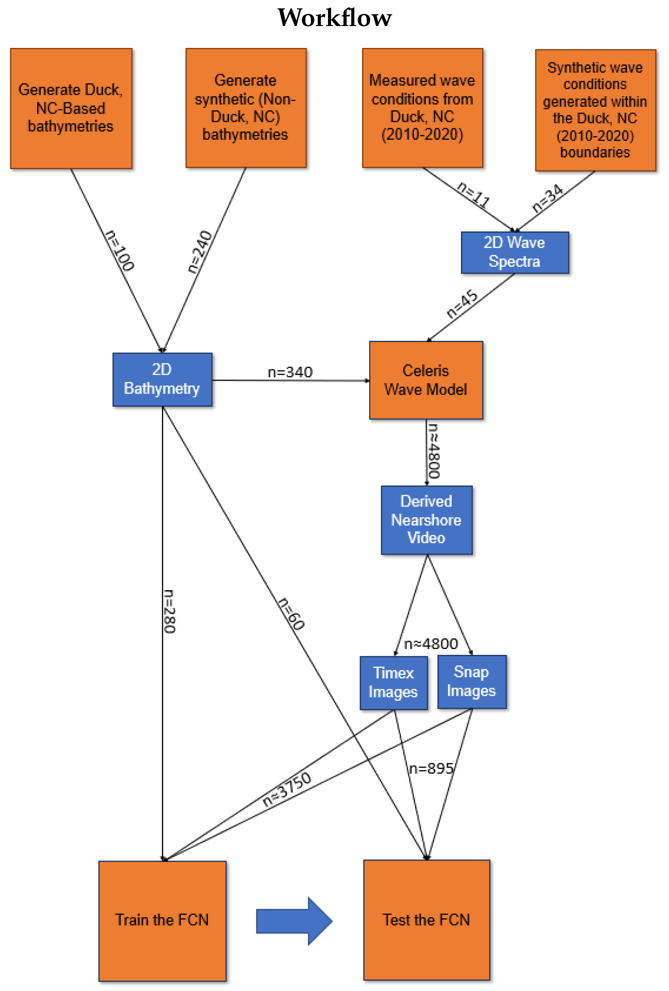
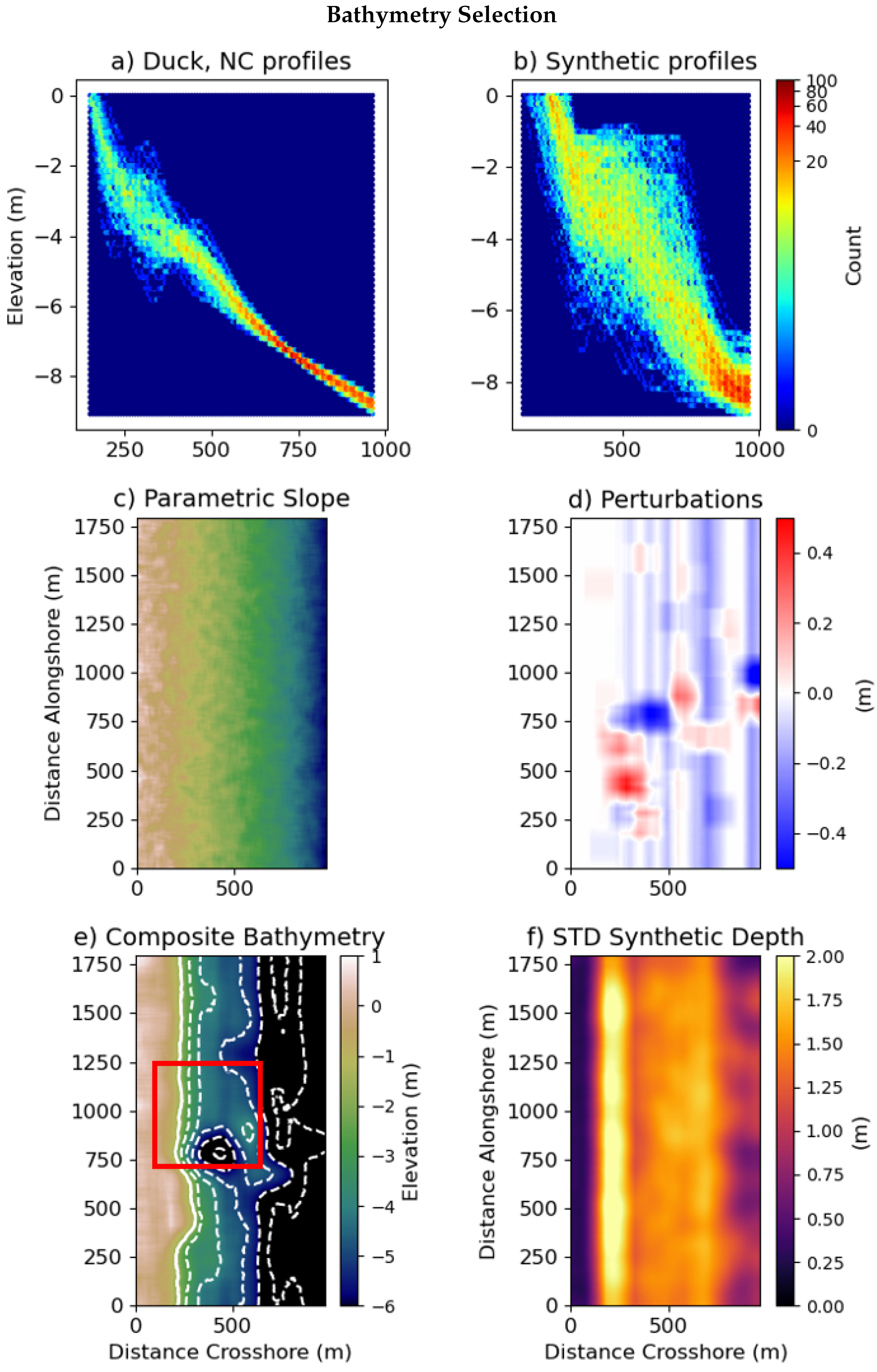
2.1. Synthetic Imagery Generation

In this work, realistic-looking synthetic sea-surface imagery was generated using a wave model to approximate the images commonly collected through typical coastal imagery methods [33,86]. Specifically, the Celeris wave model [52] was used to generate and record video of model output in the nearshore area. Celeris is an open source, phase-resolving extended-boussinesq wave model that is computed and rendered on the GPU allowing for real-time visualization of the simulated sea surface. Celeris generates and visualizes wave shoaling, refraction, reflection, and breaking, which are the relevant physical processes that influence the visual expression of wave propagation in the nearshore. Lighting effects to enhance the photo-realism of the waves use the Fresnel equations to simulate the look of the water surface (e.g., shading on the wave crest). For this effort, the sun projection was disabled and only ambient lighting from the shoreward direction was used. The “ocean” skybox was selected, which does not contain any clouds to alter the reflections from the lighting, and the foam visualization decay parameter was adjusted to more closely resemble the Argus imagery. While the position of the “camera” or view angle can be varied within Celeris, we chose to set the camera to have a direct nadir view, removing any projection artifacts that may occur in real imagery collected from a tower or with a UAS (Unmanned Aircraft System).
The Celeris model domain is 970 m in cross-shore by 1805 m in the along-shore with a computational resolution of 1 by 1 m. The model is run over a 30-min period, with 10 min being used as model spin-up time (to reach a semi-steady sea state) followed by 20 min of recording time. Single frame ‘snapshot’ images can be extracted from the model output, and averaged in time to produced a timex image. An example snapshot image from the video recording used to generate the timex images is shown for Celeris (Figure 2a) and from the ARGUS tower camera system [33] in Duck, NC (Figure 2b). While it is unlikely to find an exact replication of the observed imagery from an individual snapshot image of Celeris (specifically the exact wave and breaking patterns, since the wave boundary conditions lack phase information), the synthetic snapshot shows surficial expressions of propagating and breaking waves across the domain that are similar to geo-rectified snapshot images from the ARGUS camera system at Duck, NC. Similar to prior work, which showed synthetic timex images generated by this approach were comparable to UAV-derived coastal imagery [81], timex images generated from Celeris (Figure 2c) are reasonable approximations for timex images recorded from Argus (Figure 2d). Increases in brightness from wave breaking occur in similar locations over the sandbar and at the shoreline (Figure 2e). The Celeris imagery is thus a reasonable, though idealized, approximation of the example real Argus imagery. Notably absent in the synthetic imagery are sources of noise, such as the lighting variations seen in the real Argus imagery between two cameras (i.e., Figure 2b,d). In addition, because of the nadir view, the wave fronts do not have the same lighting characteristics as may be traditionally seen in tower or UAS-based imagery collected from the shore. Because of these differences between the synthetic and real imagery, the network developed in this effort will not be immediately applicable to real imagery without the addition of a transfer learning process or more variable and complex synthetic training data.
To simulate the wave field for an area of interest the model requires two main inputs: the bottom boundary condition (bathymetry) and the offshore wave boundary condition. Two types of bathymetries were used for this work. The first was based on 40 years of historical measured data from the U.S. Army Engineer Research and Development Center’s Field Research Facility (FRF) in Duck, NC, USA [87]. Specifically, a spatio-temporal covariance matrix was generated from the the FRF survey data and then an Empirical Orthogonal Function (EOF) approach [88] was used to generate samples of a pseudo-random bathymetry (Figure 3a). We generated 80 of these bathymetries for training, 10 for validation, and 10 for testing. The second type of bathymetries were introduced in order to mitigate the risk of over-fitting to the Duck, NC site and represent other possible coastal environments. We created 240 completely synthetic bathymetries with a 160/20/60 training/validation/testing split. The first step in creating these bathymetries was to generate a parametric cross-shore slope, for which we used typical beach-face slopes for sandy Atlantic beaches (0.01–0.1 (m/m)) (Figure 3b). Secondly, a perturbation map was added with cross-shore variability in the form of sandbars and troughs. Additional along-shore non-uniformity was added by the introduction of positive/negative cone-like features of varying location and radii (Figure 3c). The perturbation features added to the parametric slopes were sampled from a uniform random distribution for their number, location, and magnitude. The resultant bathymetry was then smoothed to produce a final bathymetric boundary condition (Figure 3e). This process yielded more complex bathymetries than in previous work [80,81].
The offshore wave boundary condition is described using TMA spectra [89,90] generated using bulk input parameters of significant wave height ( H s ), peak wave direction ( D m ), and peak wave period( T p ). A 10-year period (2010–2020) of wave conditions measured at the 8-m water depth pressure sensor array located in Duck, NC, was analyzed to develop a regional wave climatology. The most commonly occurring directions, (−17 < = D m < = 32 relative to shore-normal), and peak periods, (5 s < T p < 11 s), were combined with significant wave heights between 0.7 and 2.5 m to generate a range of offshore wave boundary conditions. These wave spectra, while not all encompassing, contain wave conditions that would likely occur on U.S. East Coast beaches. Additional bulk parameters ( H s , D m , T p ) were then generated by sampling within the bounds of the historically most common occurring wave boundary conditions described above (0.7 < H s < 2.5, −17 < = D m < = 32 , 5 s < T p < 11 s) using a Latin hypercube sampling approach [91]. This yielded a total of 45 wave conditions (11 historical aggregate, 34 created). To generate the training/validation data sets, the wave model was run using every combination of the 340 (100 Duck, NC, based, 240 fully synthetic) bathymetries and 30 of the wave conditions described above. The remaining 15 wave conditions and 80 bathymetries were used to create the test set.

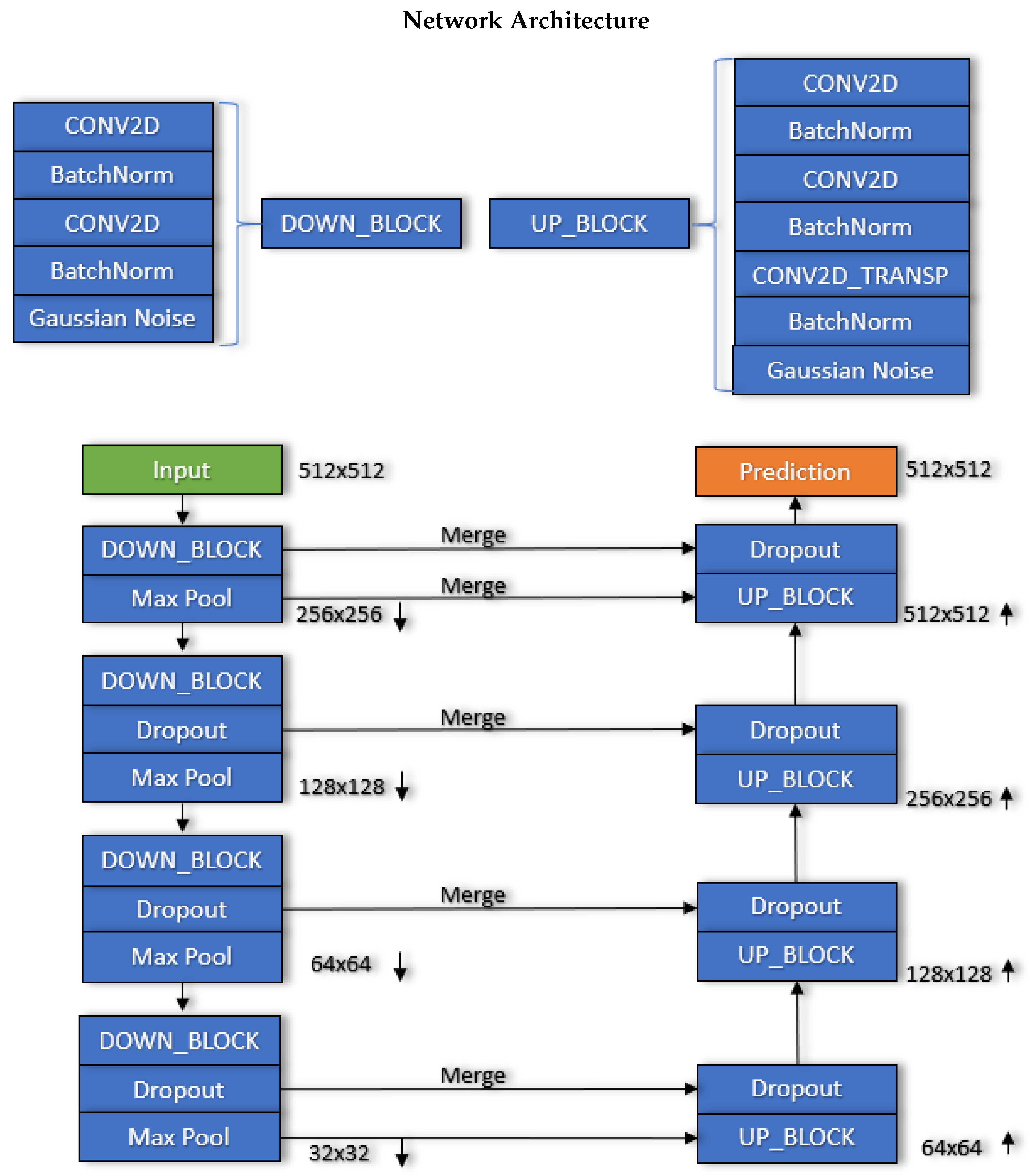
2.2. Network Architecture

Three separate fully convolutional neural network models (FCNNs) using the same architecture were trained by using different combinations of the above described image input features (timex only, snapshot only, timex and snapshot). Wave dissipation features that are present in timex imagery have shown promise in being able to estimate bathymetry by using a variety of approaches [43,80,81,92,93], but those methods are limited to situations where video imagery of the surf-zone is available for a specified duration to create the timex image. To help extend the developed networks’ capability to situations that cannot afford dwell time, we explored training an FCNN on snapshot imagery only, as well as a combined version with both snapshot and timex imagery. Timex imagery reflects time-averaged surf-zone conditions and provides information on wave dissipation close to shore, however it may lack information in deeper parts of the domain and in the trough. In contrast, snapshot imagery provides details on wave refraction and wavelength across the domain, adding value in deeper regions, but may lack spatially expansive dissipation information due to the limitations of being an instant in time. The wavelength and direction information contained in the shape of the wave crests have previously shown promise in estimating simple synthetic bathymetries [66]. Adding this type of information to the previously described timex-only work [80,81] could increase skill in areas where there is little-to-no wave breaking (trough and seaward of the sandbar) in the timex images alone. This approach would be similar to that of Beach Wizard, which combined dissipation and celerity information to best estimate bathymetry [43].
Figure 4 shows the chosen network architecture for the FCNN. The network is similar to the U-Net architecture [94], which which can incorporate information from large scales while preserving fine-scale details. A U-Net variant was used in our previous work [80,81]. While different versions of the model are trained and tested utilizing differing sets of input features, the general structure of each version remains the same. Input features are in the shape of (512, 512, # of channels), where the channel number will differ by which input features are being used (timex, snapshot, or both). While larger input sizes is desirable, hardware limitations did not allow for larger input image sizes than 512. These features are input into the network producing a (512, 512, 1) shaped depth map that corresponds to each pixel of the input channel. Skip connections, shown by the horizontal arrows labeled ‘Merge’ in Figure 4, are used to bring in high-level features from the down-sampling layers into the up-sampling layers to aid in the placement of the depth features. The current architecture has a total of 1,078,915 (1,075,971 trainable) parameters, which is approximately 4% the size of the 512 × 512 variant of the U-net architecture. Monte Carlo dropout [77,78], batch normalization [95], and uniform Gaussian noise layers are added in between each convolutional block in both the down-sampling and up-sampling side of the architecture. The batch normalization layers only affect activations during training (testing is done with a batch size of 1), while dropout is active during both training and testing similar to [78]. The uniform Gaussian noise layers shown in the down and up block defined in Figure 4 is active only during inference and is used to add a random value to the activations coming out of each convolutional block.

2.3. FCNN Model Uncertainty

The dropout and Gaussian noise layers act during testing to produce varied outputs from consistent input, allowing for the same input image to be run through the network multiple times during inference to create an ensemble of predictions to identify areas of high volatility in the predicted depth map [74,96]. Different values and locations for the dropout layers, as well as different arrangements of Gaussian noise, during inference were tried within the network to aid in estimating the uncertainty of the model. These varied in implementation, such as only having dropout/noise at the beginning, at the middle, and at the ends of the network and various combinations of the above.

2.4. Training

Training was performed using 3754 images created from the combination of 260 (80 of the 340 created bathymetries were set aside for testing) bathymetries and 30 wave conditions. During training, the loss function value was checked on a validation set consisting of 350 images that were set aside from the training set. The loss function was minimized using the NAdam [97] optimizer with default parameters including a starting learning rate of 10 3 . After 75 epochs, the learning rate was annealed to 10 4 . Convergence was defined as the point where the loss of the validation data set did not decrease after 10 consecutive epochs. Additionally, different optimizers, including stochastic gradient descent (SGD) and Adam were tried, while varying the learning rate. A more fully exhaustive search across all possible hyperparameters could reveal improvements in test set accuracy, but similar results from past work [80,81], as well as the breadth of approaches tried here, initially imply a lack of sensitivity of the model to modest changes in either architecture or hyperparameters.

3. Results

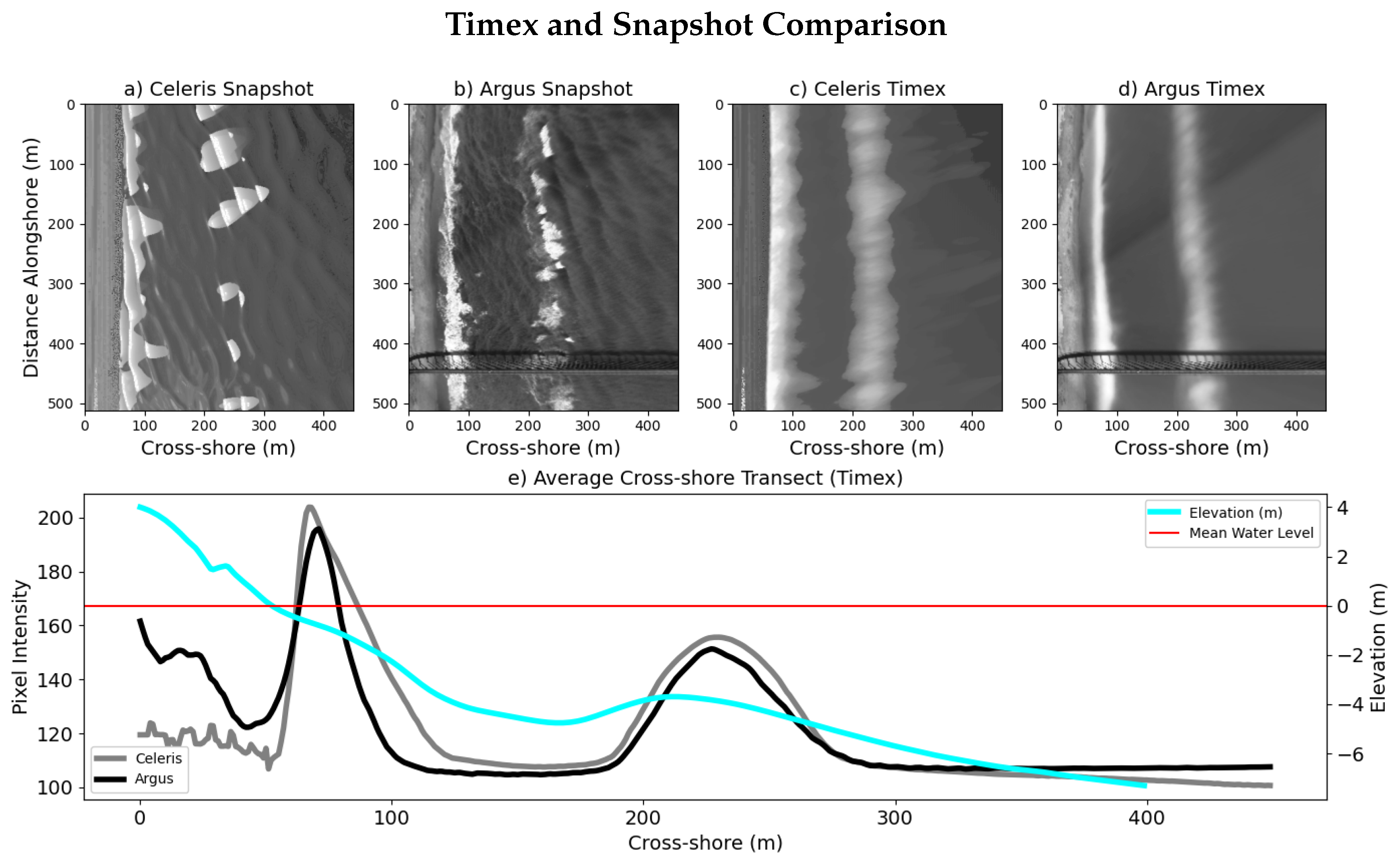
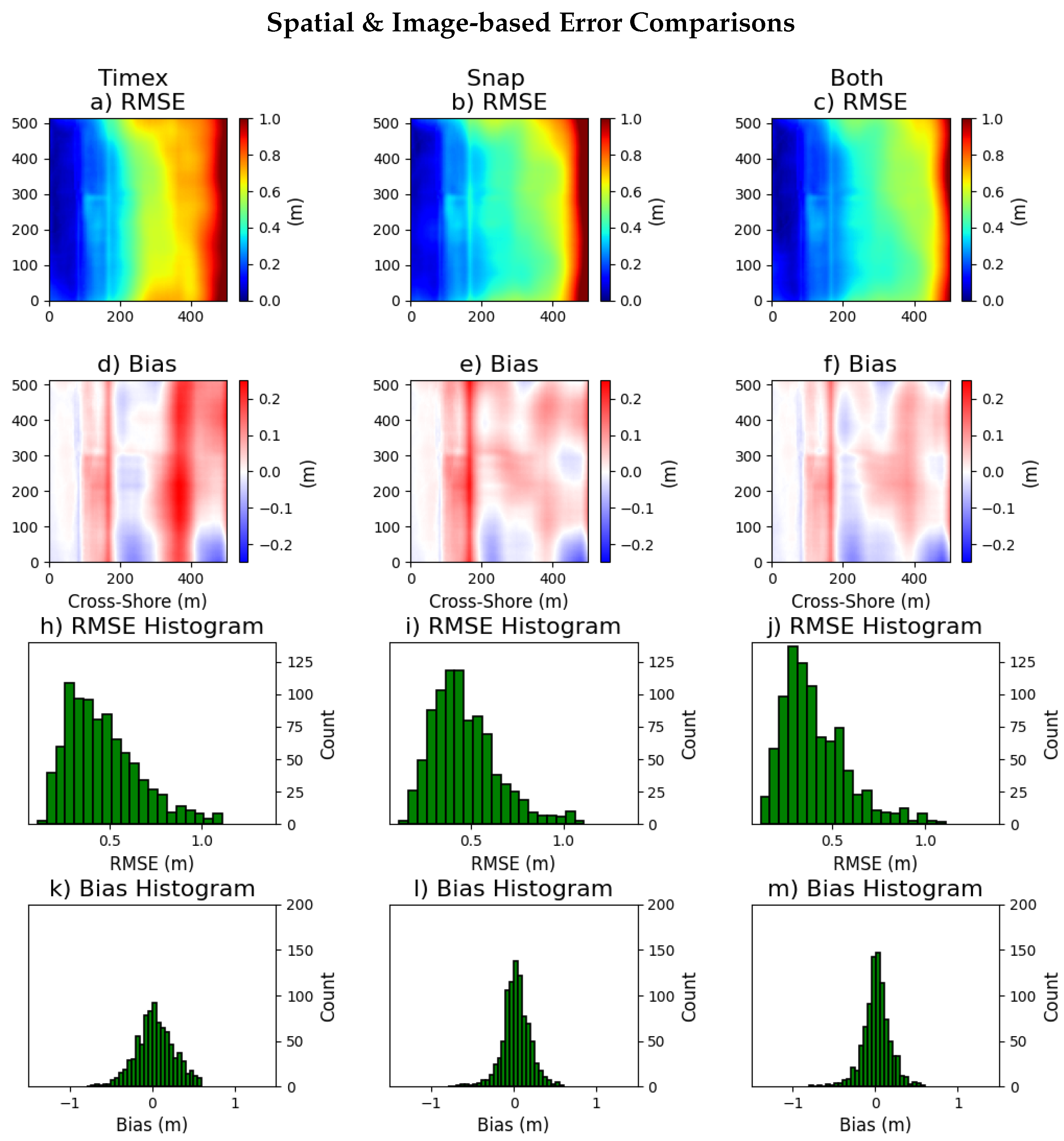
3.1. Input Feature Comparison

Figure 5 compares an example of the model output from the three network setups: timex only (first row), snapshot only (second row), and timex and snapshot (third row). All three versions of the model are able to predict the shoreline and location and magnitude of the shore-parallel sandbar well. The timex-input only FCNN (Figure 5a) predicts the worst mean ensemble bathymetry between the three methods for this example, by predicting the trough to be much too deep. The increased error appears primarily in the regions without much wave breaking, where the imagery lacks visible signatures related to depth (cross-shore position 200–350 m). The snapshot-only FCNN (Figure 5e) predicts a better mean bathymetry (Figure 5b) and has less spread in the predictions than the timex-only version (grey lines in Figure 5d,h). The combined FCNN (input is both the timex and snapshot images in Figure 5a,e) has the best agreement between truth (Figure 5i) and predicted bathymetry (Figure 5j) with a reasonable uncertainty interval from the estimation ensemble.
In Figure 6, spatial variability in summary statistics (root mean squared error (RMSE), Figure 6a–c; bias, Figure 6d–f) from the three FCNNs across the entire test set (895 images) are evaluated. A decrease in RMSE is shown between timex (Figure 6a) and snapshot-only inputs (Figure 6b), particularly offshore of 200 m cross-shore. RMSE is further decreased when using both images as inputs (Figure 6c). Biases drop in magnitude from Figure 6d–f, as the input changes from timex only, to snapshot only, to both timex and snapshot. While the greatest improvement in performance was shown when utilizing snapshot only instead of timex only, the FCNN that utilizes both inputs demonstrates advantages over each input data set individually. Notably, the RMSE and bias are reduced in the center of surf-zone in the same areas as the snapshot only FCNN. Additionally, the combined FCNN includes the lower RMSE found in the timex-only (when compared to snapshot-only) in the furthest regions offshore. Histograms of image-wise RMSE (Figure 6h–j) and bias (Figure 6k–m) help elucidate these differences. Specifically, the combined FCNN (Figure 6j) has fewer images in the high RMSE bins, when compared with the snapshot-only and timex-only FCNN, indicating that this network has fewer extreme mis-predictions.
The example model output shown in Figure 5, as well as the error statistics over the test set shown in Figure 6, demonstrate similar trends to the overall statistics reported in Table 1. Specifically, mean absolute error, RMSE, depth-normalized RMSE, and the 90-th percentile error across the entire test set decrease from the timex-only network, to the snapshot-only network, to the network trained on both inputs (Table 1). Bounded pixels also increase with increasing information. A pixel is defined as “bounded” when the truth depth falls within the uncertainty range at a given pixel. For the remainder of the paper, the focus will shift to analysis of the the FCNN that includes both inputs, given its superior performance relative to the other networks.

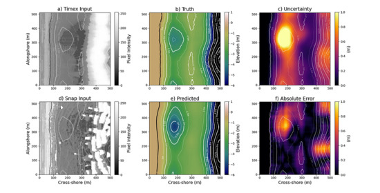
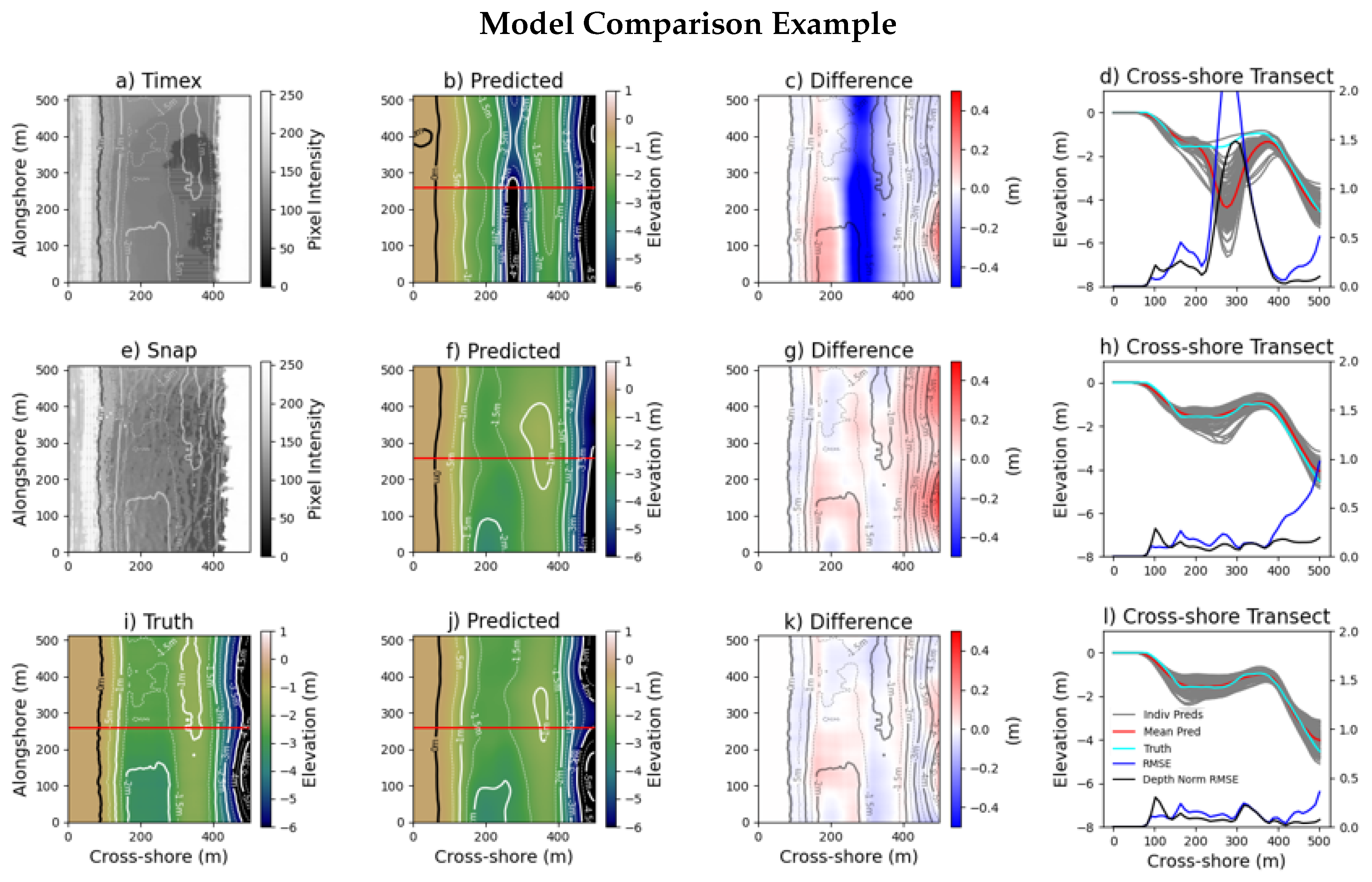
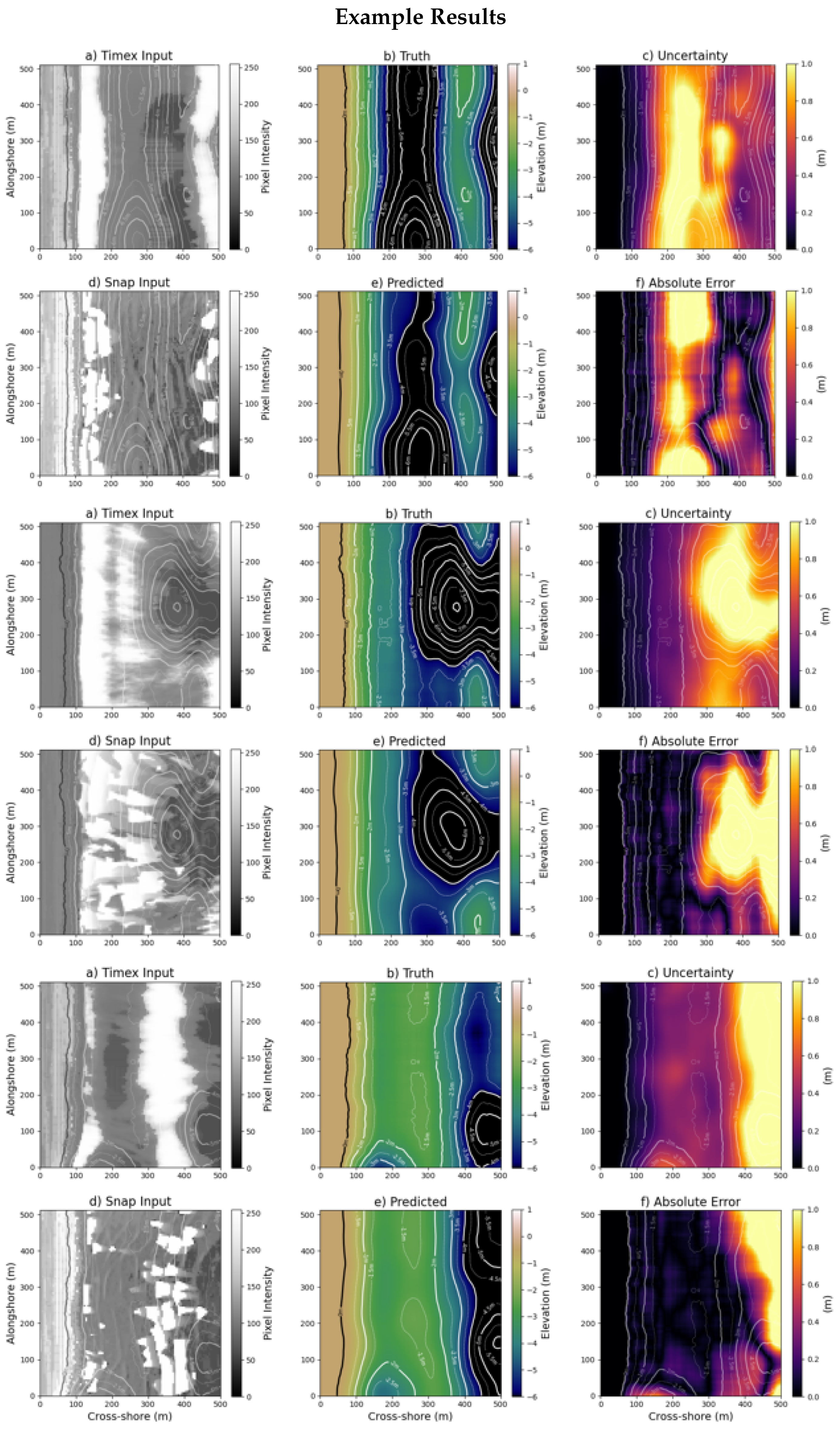
3.2. Example Predictions

Example results showing the broad applicability of the combined FCNN to three unique bathymetric profiles are shown in Figure 7 with a comparison of estimated model uncertainty and true error. In the first case (Figure 7a–f), there is significant wave breaking over a bar at the outer portion of the domain and at the shoreline (cross-shore position 475 and 150 m, respectively, Figure 7a,d). No wave breaking is visible in the large trough (cross-shore positions 200 to 385 m) between the shoreline and bar (shown in Figure 7a,b); however, the wave refraction information in this area introduced by the snapshot input (Figure 7d) allows for accurate predictions in the trough (Figure 7e). Spatial maps of the 95th confidence interval of the ensemble range at each pixel location are used to characterize spatially variability in model results Figure 7c. In this example, the model performs well, qualitatively placing the trough and sandbar in the correct cross-shore position, as well as estimating the sandbar depth. Errors are greatest in the deepest parts of the trough, which are underestimated by ≈1 m, but bounded by the 95th confidence interval of the ensemble spread.
In the second example (Figure 7a–f, rows three and four), there is a large depression in the center of the domain, similar to a rip channel. In the timex input, there is little wave breaking in the deepest portions (cross-shore position 300 to 475 m, along-shore position of 100 to 500 m). Wave breaking does occur over the sandbar found at the far northern and southern portions of the image, and again at the shoreline. Overall the model performs well, correctly characterizing the overall morphology of the bathymetry. The trough is correctly located, as well as the shallow split sandbars at the north and southern parts of the image. The inner-surf zone bathymetry is also well represented. The highest errors (near 1 m) are found in the deep depression (Figure 7l). The uncertainty estimation (Figure 7i) correctly shows higher expected error in this location but does not show sufficient uncertainty in the far seaward edge (cross-shore position 485+ m) to bound the observed error. Interestingly, the FCNN predicts too shallow of a trough in this region, suggesting that a rip current circulation pattern may be artificially shortening the wavelengths (slowing down incoming waves) in this region.
The third example (Figure 7a–f, rows five and six) shows results on a more dissipative bathymetric profile with a shallow shore-attached sandbar in the inner surf-zone. There is a large amount of dissipation at the steeply sloped edge of this bar, where the depths becomes very shallow (cross-shore position 350 m), with minimal wave breaking at the shoreline. In the snapshot image, refracting and breaking waves are clearly visible across the domain. In this example, the model errors are less than 0.2 m across most of the domain, with the exception of the offshore region in the northeast corner of the domain. Interestingly the model estimates moderate uncertainty over the shallow sandbar despite the low error in the prediction (Figure 7). The ensemble spread is highest at the furthest offshore portion of the image, and this correlates with increased error when compared to ground-truth. The model incorrectly estimates the depth in most of the area seaward of the sandbar (cross-shore position 400–500 m), with errors of 0.5 to 1 m found in the northern portion of the image where the model is biased too shallow.
Overall, the model performance is satisfactory (RMSE = 0.39 m) across a range of synthetic morphological states and wave conditions. While uncertainty estimates do not correlate precisely with observed error, they frequently bound the true depth with the 95th confidence interval of the ensemble spread and can be used to visually identify regions with increased error.
The FCNN’s ability to bound true depth errors with its predictive uncertainty over the entire test set is assessed in Figure 8. The FCNN’s predictive uncertainty bounds at least 60 and often more than 80 percent of the predictive error for each location across the test set beyond the 100-m cross-shore position (Figure 8a). Regions of the domain that are typically beach pixels are bounded with less frequency. Specifically, onshore of 100-m cross-shore location, the number of test images with underwater pixels in this region decreases to 20% or less of the entire data set (Figure 8b). As a result, smaller sample sizes may affect the statistics calculated in this region.
In Figure 8c–e, pixels at which the estimated uncertainty bounds or fails to bound the true value are assessed as a function of depth, absolute error, and bias. Since most pixel errors are frequently bounded by the uncertainty estimate ( 88%, Table 1), the number of bounded pixels (green) will almost always outnumber unbounded pixels (blue) in these histograms. At almost every depth the bounded pixels outnumber the unbounded pixels (as expected), with the exception of near the extreme values, where the most shallow depths (less than 1 m) see almost as many unbounded pixels as bounded. In addition, the deepest depths (more than 8 m) tend to be unbounded by the ensemble of predictions (Figure 8c). As absolute errors for individual pixels increase beyond 1.0 m (Figure 8d) and biases increase beyond ±0.75 m (Figure 8e), the histograms indicate pixel errors are more often unbounded than bounded, suggesting our uncertainty intervals are often not bounding our largest errors.

4. Discussion

Inference results over the test set (Table 1) show errors on the scale of 10% of the water depth across 90% of the domain for a range of synthetic bathymetries, demonstrating promising results using an image-based FCNNs to estimate bathymetry. The scale of errors using our FCNN approach is comparable to prior bathymetry inversion approaches. It is important to note that these techniques were assessed on real imagery, not synthetic imagery, so there are additional potential sources of error that may be relevant to the FCNN performance on real imagery, not addressed by this current study. Other approaches have found similar scale errors (RMSE = 0.40 m) using dissipation (timex) techniques [42]. Numerical modeling techniques for inversion that combine dissipation information, as well as wave celerity information from radar [43], see RMSE between 0.3–0.5 m. cBathy [26], an approach that utilizes video of the surf-zone to derive wave celerity and then perform linear depth inversion, typically sees RMSE around 0.51 m after observing wave speeds for an average of 33 h. Additionally, during higher, non-linear wave conditions, video-based linear dispersion inversion approaches can overestimate the depth by up to 2.0 m and have difficulty locating the cross-shore position of the sandbar [35,44]. Recent approaches using satellite image sequences to extract wave celerity see RMSE of around 1.4 m [14]. One advantage of using synthetic imagery is the ability to test the algorithm’s performance over a large and varied ensemble of synthetic bathymetries, exceeding the amount and variation of measured high-resolution bathymetric data sets. The RMSE of our ML approach rarely exceeds 0.68 m (90%) for any given subaqueous pixel, with a total RMSE of 0.39 m across all subaqueous pixels. Additionally, this image-based ML method requires fewer pre-processing steps [26,43] or manual inputs [93] than the similar methods. However, training the neural network is time consuming (around 20 hours with both inputs), and identifying the reasoning behind some errors is difficult. In addition, our results only include performance statistics on idealized synthetic imagery. Once trained, the network has a significantly decreased inference time (∼37 ms) relative to direct inversion techniques, that can take minutes to run [26], or compared to model-based inversion methods that rely on solving differential equations during run-time to produce a bathymetric estimate [36,38,39,43]. Additionally, the snapshot-only version of the trained FCNN can utilize only a single snapshot of sea-surface imagery, removing the requirement for a time-series (video) of images of the surf-zone, with only a small reduction in overall error over the test-set.

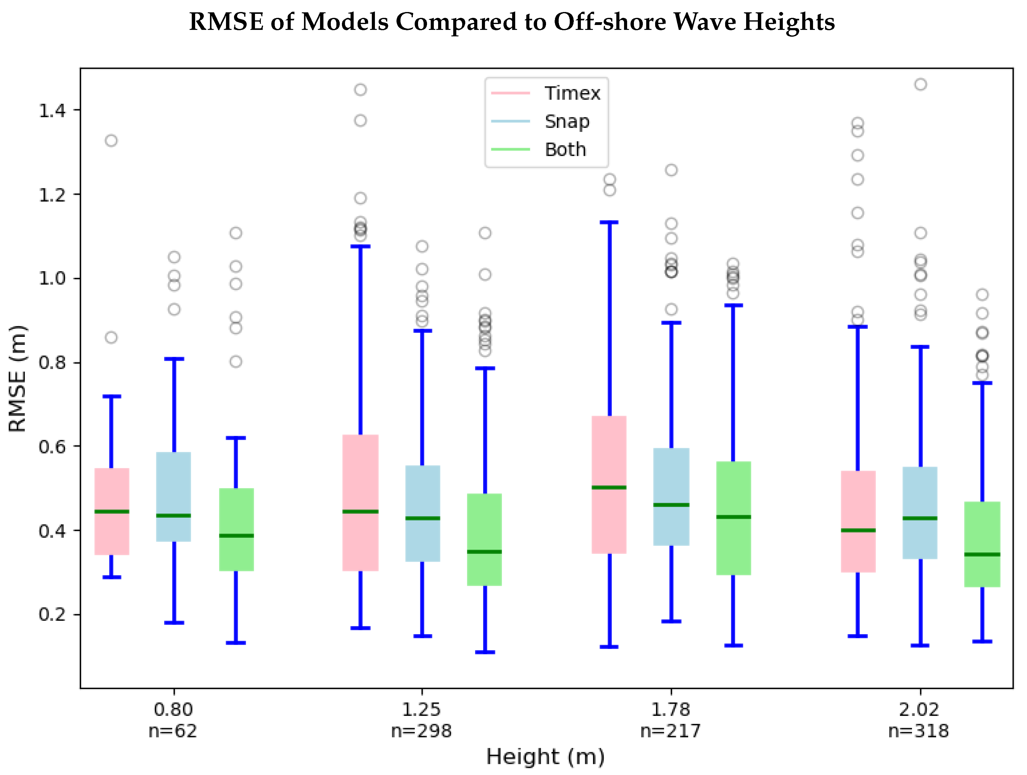
4.1. Wave Conditions

Methods that extract wave celerity from image sequences tend to see increased error during larger wave heights, which is when the linear shallow-water wave equations cease to accurately describe wave propagation in the surf-zone, and when breaking can interfere with the celerity extraction algorithm [44]. Methods that use timex-based algorithms see opposite trends, with increased errors when wave heights are small [43]. In this effort, we tested the FCNN in significant wave height conditions ranging from 0.7 to 2.5 m, and observed no significant trends in performance with wave height (Figure 9). This is in contrast to the physics-based approaches, which see wave-height dependent performance, potentially due to simplifications in the underlying physics of the models [26]. At this time, it is unclear if the lack of wave height dependence on the accuracy of our FCNN is because it has “learned” some of the non-linear relationships between wave breaking and wavelength in shallow-water, or if we did not test over a broad enough wave climate to observe these trends. For the test set wave conditions, the “both input” FCNN performed better than snapshot-only or timex-only in every wave height scenario (Figure 9), which may be due to the combination of information from energy dissipation and wavelength. The timex-only FCNN almost always had the highest groups of RMSE outliers, which suggests that the lack of wave structure information (only included in the snapshot imagery) can lead to unreasonable predictions. In addition, we found little-to-no significant trends between peak wave period and direction and error in the predictive model (not shown). A larger set of wave conditions, with more extreme wave energies is of interest for future work.

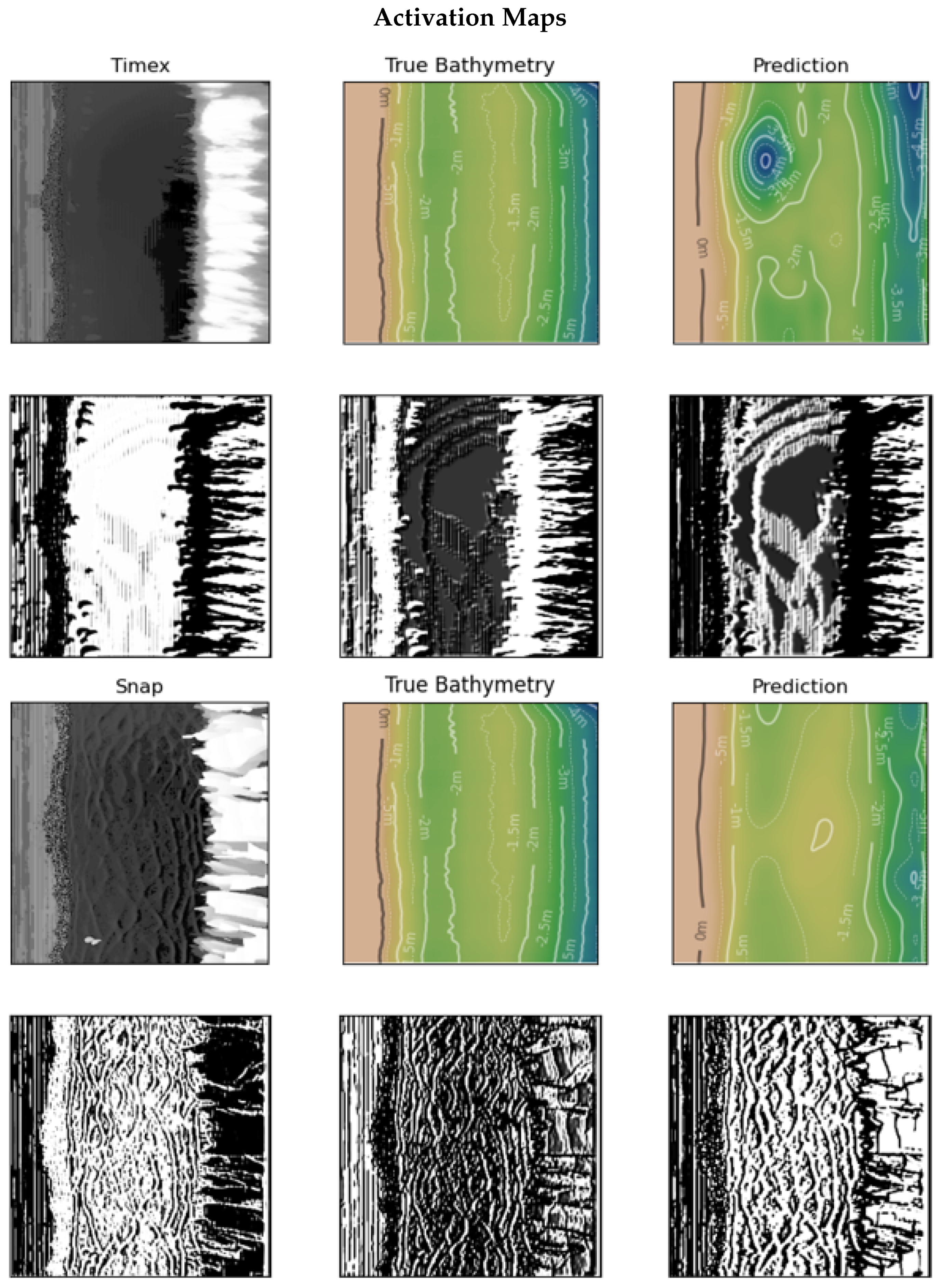
4.2. Activation Maps

Inference activation maps [98,99] are often used to identify the input features in the image which the FCNN keys onto during training and prediction. These maps highlight the intensity of individual neurons in different layers of the network, and can be used, alongside the input features, to see which aspects of the input features are involved in prediction. Thus, we can use activation maps to provide insight into what information the FCNN is using during training.
In Figure 10, results from the timex-only and snapshot-only trained FCNN are shown for the same wave and bathymetry combination alongside three example activation maps. Activations from the timex input (Figure 10, second row) reveal the lack of information in the areas with little wave breaking, such as in the trough. In this area, the activations across the network become sensitive to extremely small changes in lighting gradients. These lighting gradients could be reflective of differences in wave steepness across the domain or may be completely unrelated to the bathymetric gradients. The network incorrectly infers a depression in the trough to explain the apparent lack of breaking. This type of error in the trough, and in other areas that lack the wave dissipation information (pixel intensity gradients) in the timex images, confirms the potential benefit of including snapshot imagery that contains more information in these regions in the form of refracting waves in the input features. Snapshot imagery activations (Figure 10, fourth row) highlight the FCNN model’s ability to extract wave structure information from areas with little wave breaking. The snapshot-trained FCNN is able to identify wave structure patterns, which the activation maps indicate are providing increased information in the regions with less wave breaking when compared to the timex-only activation maps. As a result, the snapshot-only FCNN infers a more accurate depth in the areas where there is little wave breaking. This implies the decrease in wavelengths as waves move into shallower water, combined with wave refraction information (bending of the wave crests around bathymetric features) provides information the FCNN uses to make the bathymetric prediction, similar to approaches used by short-dwell satellite-based inversion methods [15].
The relative closeness in errors shown in Table 1 between the snapshot-only and both FCNN, suggests the expression of wave dissipation in the timex images is rarely adding much extra information to the predictions. However, some examples, such as the one shown in Figure 6, demonstrate where the timex image can provide additional information relative to snapshot-only—in this case the increased continuum of wave breaking at the offshore boundary decreases the RMSE and bias in this region. Therefore, if available, the input of both a dissipation proxy (timex imagery) and wavelength proxy (snapshot imagery) to the FCNN provides a better estimate of depth, which has also shown to be the case with other approaches [43]. Different environmental variables and/or bathymetric profiles may provide more opportunity for timex images to add more information, such as on lower sloped, dissipative beaches where gradients in dissipation may be wide-spread. However, the success of the snapshot-only model demonstrates the ability of the ML algorithm to learn relationships between changes in depth and the resultant wavelength changes previously exploited in the very first depth inversion approaches and state of the art satellite methods [14,15,27,66]. From a practical perspective, getting similar errors between the snapshot-only and both FCNNs is a good thing; single snapshots of the surf-zone are logistically easier to collect and more widely available than taking high-quality 20-min video imagery. For example, the success of snapshot implies that this synthetic data could be exploited in transfer learning for domain adaption to data similar in appearance, such as satellite imagery or limited-dwell, high-altitude aerial imagery, in future works.

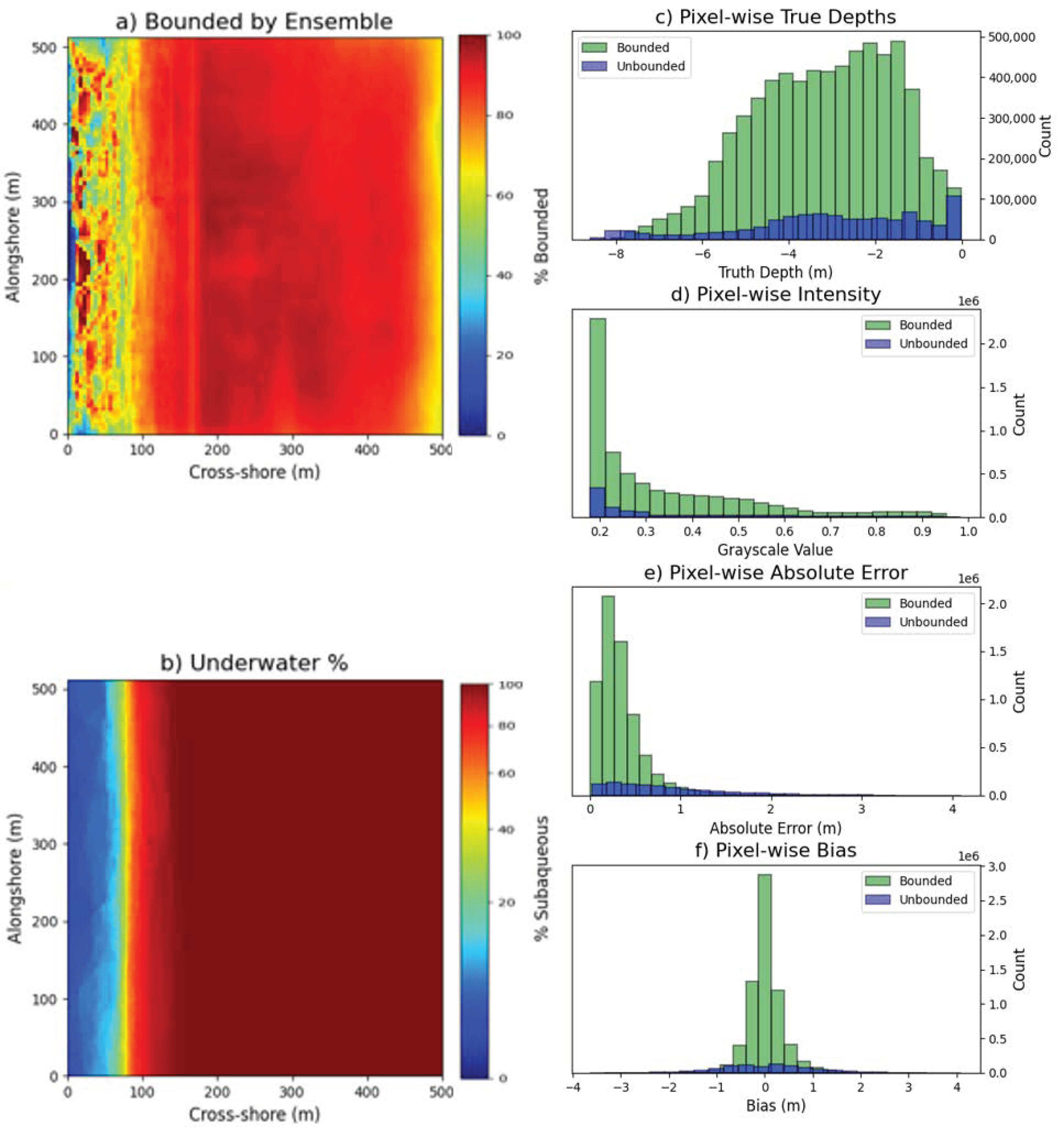
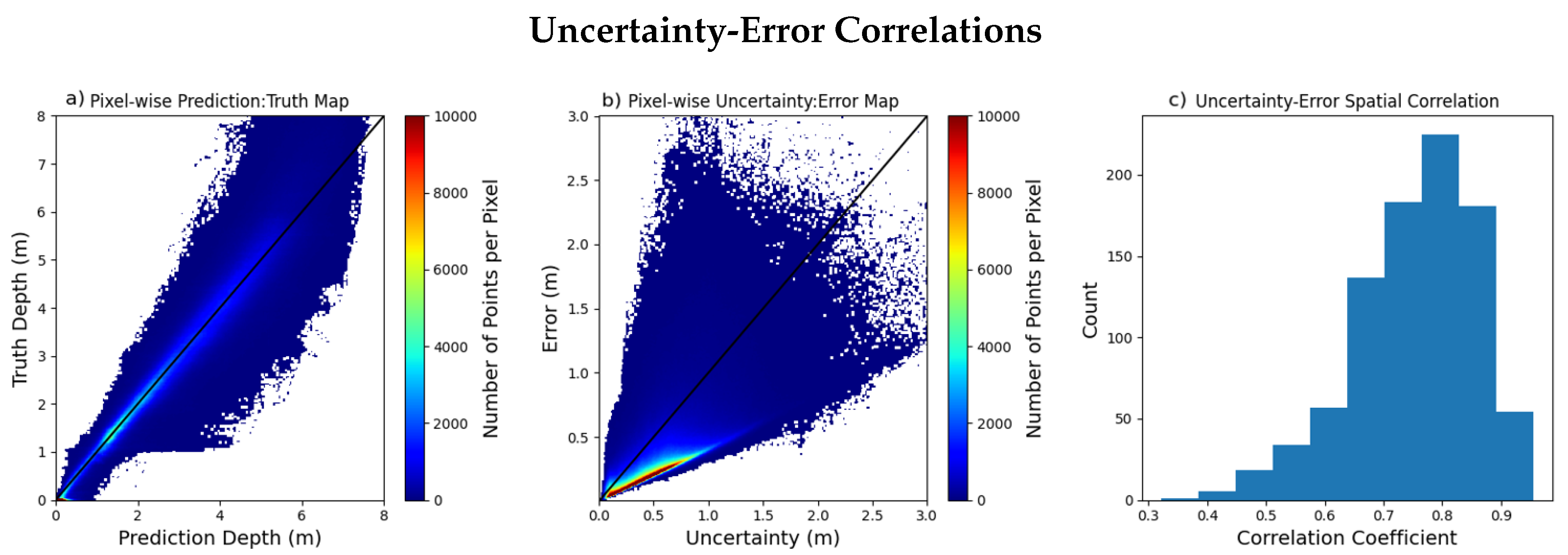
4.3. Uncertainty Measurements

Various methods to estimate model uncertainty are applied to the neural network in the form of MC-dropout, infer-transformation, and infer-noise. This creates the uncertainty maps shown in Figure 7. The FCNN’s 95% confidence interval bounded observed error 88% of the time over the entire test set (Table 1), and magnitudes frequently corresponded with observed error (Figure 8). Relative to other video-based bathymetric inversion methods, such as cBathy [26], which bounds errors around 50% of the time, these results provide higher fidelity uncertainty estimates. In addition the location of higher errors often corresponded with regions with less information in the input imagery (i.e., less wave breaking or fainter wave refraction patterns), which is where we expect the algorithm to perform more poorly (Figure 8e). Figure 11a shows a pixel-wise 1:1 plot of the prediction and truth depth, showing strong agreement that reflect low error values seen across the test set Table 1. Figure 11b shows a pixel-wise 1:1 plot of the uncertainty and observed absolute error. Pixel uncertainties tend to increase for pixels with larger observed error; however, our estimated uncertainty tends to exceed the actual algorithm error, which makes sense since our uncertainty estimate provides a 95% confidence interval. Spatial correspondence between error and uncertainty maps (see Figure 7 for examples of the 2d error and uncertainty maps being discussed), is high, with a median correlation coefficient of 0.78 between each uncertainty map and error map in the test set (Figure 11c). The strong performance of our uncertainty estimates at each grid cell allows prediction of when the FCNN inference is useful by giving a spatial estimate of error for each image. This can aid in actionable decision-making where high risk is unacceptable (such as for navigation of vessels).

4.4. Future Work

This work has focused on exploring whether an image-based ML approach can be successfully implemented to infer bathymetry from timex and/or snap imagery, and thus has used a simplified form of synthetic data that, while, in general, agrees with the features seen in remotely sensed imagery, still lacks the robustness to various types of real-world noise that are present in remotely sensed imagery. Because of this, immediate goals include both expanding the existing synthetic data set, as well as transitioning to real-world remotely sensed imagery using transfer learning for domain adaption. That is, immediate goals will be to train on a fully robust synthetic data set that mimics remotely sensed data as close as possible, and then to fine-tune the FCNN on much smaller sets of high-resolution real imagery matched with their bathymetric survey pairs. Creating this robust data set will involve several additions to the existing data set that can be categorized into two subsections: (1) expanding the wave characteristics; and (2) accounting for sources of noise in real imagery, such as lighting variations, weather conditions, or rectification/projection errors. Expansion of the wave conditions will include testing of an increased range in wave heights and periods, as well as include variations in directional spread of the input spectra. To more closely mimic remotely sensed data, lighting conditions will be varied in the Celeris model to account for various lighting conditions from different sun angles and intensities. In addition, analysis of the types of noise in real imagery is presently being conducted to identify the relevant factors, such as weather conditions or ortho-rectification/projection errors, which may affect the output performance of the FCNN. Additionally, image decomposition techniques to reduce synthetic and remotely sensed imagery to a more common component structure to more easily utilize the transfer learning for domain adaption is also being explored.

5. Conclusions

A 2D FCNN was used to estimate nearshore bathymetry from time-averaged and snapshot synthetic imagery, as well as on a combination of both image types. The FCNN that utilized both image types had the lowest RMSE over the test set (0.39 m) though the snapshot only model’s RMSE was similar at 0.44 m. The FCNN was tested over a wide range of highly variable synthetic bathymetries, with a best RMSE prediction of 0.11 m and a median RMSE of 0.37 m. These results demonstrate the promise of using a 2D FCNN to estimate nearshore bathymetry from time-series and snapshot synthetic imagery of the surf-zone. The relative success of snapshot only imagery, which contains wave refraction information along with some dissipation, bodes well for the algorithm’s potential success with high-resolution single-frame images, reducing the reliance on dwell of many common bathymetric inversion algorithms. Unlike existing physics-based inversion approaches that show increased errors with higher non-linearity (when wave heights become large), the FCNN shows robustness in estimation across wave heights up to 2.5 m. Finally, the methods used to estimate model uncertainty provide a range of ensembles that usually (88%) bound the true water depth in our studies, allowing for a reasonable estimation of both location and magnitude of error at any given location in the area of prediction.

6. Source Code

The code to retrieve and bin wave conditions by their wave/height and direction is found in https://github.com/collins-frf/Wave-Conditions. Synthetic wave conditions were sampled from between highly occurring edge cases from the measured data set at the FRF’s 8-m pressure array. The code to generate the ensemble of bathymetries based on historical measurements from Duck, NC, is located at https://github.com/collins-frf/bathy_gen, while the code to generate (and plot) the synthetic bathymetries is located at https://github.com/collins-frf/Celerity_Net. The Celeris wave model is available for download from https://github.com/collins-frf/Wave-Conditions. The code to run and record the model output (using MATLAB) with the generated bathymetries and wave conditions is found in https://github.com/collins-frf/celerisDataGen. The code to create tiff files of timex and snapshot images from the recorded Celeris visualizations is found in https://github.com/collins-frf/PyTimex.
The model was trained validation and tested using mainly the Pytorch [100] and Tensorflow [101,102] libraries, with the data loading and serving handled by a modified Pytorch.Dataset class, while the model was constructed, trained, and tested with Tensorflow/Keras. The Celeris model simulations were run on a Dell Precision 5820 with 64GB of RAM and NVIDIA RTX 2080. The FCN model was trained on a custom built PC with 64 GB of RAM and a NVIDIA RTX Titan V with 24GB of VRAM.
The feature inputs used during training consisted of different inputs depending on the referenced model. Results were presented for both timex, snapshot, and a combination of both.

Author Contributions

Conceptualization, A.M.C., K.L.B., A.S.B., T.J.H., M.W.F.; methodology, A.M.C., K.L.B., A.S.B., T.J.H., M.W.F., J.L., J.W.L.; software, A.M.C., A.S.B.; validation, A.M.C.; formal analysis, A.M.C.; investigation, A.M.C.; resources, K.L.B., A.S.B.; data curation, A.M.C.; writing—original draft preparation, A.M.C., K.L.B., A.S.B., T.J.H., M.W.F., J.L., J.W.L.; writing—review and editing, A.M.C., A.S.B., T.J.H., M.W.F.; visualization, A.M.C.; supervision, K.L.B., A.S.B., T.J.H., J.L.; project administration, K.L.B.; funding acquisition, K.L.B. All authors have read and agreed to the published version of the manuscript.

Funding

This research was funded by the Assistant Secretary of the Army for Acquisition, Logistics, and Technology (ASAALT) under 0603734/T08/11 and 0603463/AS9/02.

Acknowledgments

We would like to thank Sasan Tavakkol and Pat Lynett for helping us with their wave model, Celeris, as well as the faculty and graduate students at University of North Carolina-Wilmington that provided their input and feedback on the research. Special thanks to Matthew Geheran for development of the EOF bathymetry generation function using Duck, NC, survey data.

Conflicts of Interest

The authors declare no conflict of interest.

References

  1. Birkemeier, W.A.; Mason, C. The CRAB: A unique nearshore surveying vehicle. J. Surv. Eng. 1984, 110, 1–7. [Google Scholar] [CrossRef]
  2. Dugan, J.P.; Vierra, K.C.; Morris, W.D.; Farruggia, G.J.; Campion, D.C.; Miller, H.C. Unique vehicles used for bathymetry surveys in exposed coastal regions. In Proceedings of the US Hydrographic Conference Society National Meeting, Mobile, AK, USA, 26–29 April 1999. Available online: https://rb.gy/bftf3f (accessed on 14 October 2020).
  3. Dugan, J.P.; Morris, W.D.; Vierra, K.C.; Piotrowski, C.C.; Farruggia, G.J.; Campion, D.C. Jetski-based nearshore bathymetric and current survey system. J. Coast. Res. 2001, 107, 900–908. [Google Scholar]
  4. Komar, P.D.; Gaughan, M.K. Airy wave theory and breaker height prediction. Coast. Eng. 1973, 405–418. [Google Scholar] [CrossRef]
  5. Sallenger, A.H., Jr.; Holman, R.A.; Birkemeier, W.A. Storm-induced response of a nearshore-bar system. Mar. Geol. 1985, 64, 237–257. [Google Scholar] [CrossRef]
  6. Fredsøe, J.; Deigaard, R. Mechanics of Coastal Sediment Transport; World Scientific: Singapore, 1992; Volume 3. [Google Scholar]
  7. Trenhaile, A.S. Coastal Dynamics and Landforms; Oxford University Press on Demand: Oxford, UK, 1997. [Google Scholar]
  8. Jackson, D.W.T.; Cooper, J.A.G.; Del Rio, L. Geological control of beach morphodynamic state. Mar. Geol. 2005, 216, 297–314. [Google Scholar] [CrossRef]
  9. Gao, J. Bathymetric mapping by means of remote sensing: Methods, accuracy and limitations. Prog. Phys. Geogr. 2009, 33, 103–116. [Google Scholar] [CrossRef]
  10. Holland, K.T.; Lalejini, D.M.; Spansel, S.D.; Holman, R.A. Littoral environmental reconnaissance using tactical imagery from unmanned aircraft systems. In Ocean Sensing and Monitoring II; International Society for Optics and Photonics: Bellingham, WA, USA, 2010; Volume 7678, p. 767806. Available online: https://rb.gy/ejbbmg (accessed on 14 October 2020).
  11. Holman, R.A.; Brodie, K.L.; Spore, N.J. Surf zone characterization using a small quadcopter: Technical issues and procedures. IEEE Trans. Geosci. Remote Sens. 2017, 55, 2017–2027. [Google Scholar] [CrossRef]
  12. Holland, K.T.; Palmsten, M.L. Remote sensing applications and bathymetric mapping in coastal environments. Adv. Coast. Hydraul. 2018, 35, 375–411. [Google Scholar]
  13. Brodie, K.L.; Bruder, B.L.; Slocum, R.K.; Spore, N.J. Simultaneous Mapping of Coastal Topography and Bathymetry from a Lightweight Multicamera UAS. IEEE Trans. Geosci. Remote Sens. 2019, 57, 6844–6864. [Google Scholar] [CrossRef]
  14. Almar, R.; Bergsma, E.W.J.; Maisongrande, P.; de Almeida, L.P.M. Wave-derived coastal bathymetry from satellite video imagery: A showcase with Pleiades persistent mode. Remote Sens. Environ. 2019, 231, 111263. [Google Scholar] [CrossRef]
  15. Bergsma, E.W.J.; Almar, R.; Maisongrande, P. Radon-Augmented Sentinel-2 Satellite Imagery to Derive Wave-Patterns and Regional Bathymetry. Remote Sens. 2019, 11, 1918. [Google Scholar] [CrossRef] [Green Version]
  16. Vos, K.; Harley, M.D.; Splinter, K.D.; Simmons, J.A.; Turner, I.L. Sub-annual to multi-decadal shoreline variability from publicly available satellite imagery. Coast. Eng. 2019, 150, 160–174. [Google Scholar] [CrossRef]
  17. Sabour, S.; Brown, S.; Nicholls, R.; Haigh, I.; Luijendijk, A. Multi-decadal shoreline change in coastal Natural World Heritage Sites—A global assessment. Environ. Res. Lett. 2020. [Google Scholar] [CrossRef]
  18. Eugenio, F.; Marcello, J.; Martin, J. High-resolution maps of bathymetry and benthic habitats in shallow-water environments using multispectral remote sensing imagery. IEEE Trans. Geosci. Remote Sens. 2015, 53, 3539–3549. [Google Scholar] [CrossRef]
  19. Jagalingam, P.; Akshaya, B.J.; Hegde, A.V. Bathymetry mapping using Landsat 8 satellite imagery. Procedia Eng. 2015, 116, 560–566. [Google Scholar] [CrossRef] [Green Version]
  20. Pacheco, A.; Horta, J.; Loureiro, C.; Ferreira, Ó. Retrieval of nearshore bathymetry from Landsat 8 images: A tool for coastal monitoring in shallow waters. Remote Sens. Environ. 2015, 159, 102–116. [Google Scholar] [CrossRef] [Green Version]
  21. Jay, S.; Guillaume, M. Regularized estimation of bathymetry and water quality using hyperspectral remote sensing. Int. J. Remote Sens. 2016, 37, 263–289. [Google Scholar] [CrossRef]
  22. Lin, Y.C.; Cheng, Y.T.; Zhou, T.; Ravi, R.; Hasheminasab, S.M.; Flatt, J.E.; Troy, C.; Habib, A. Evaluation of UAV LiDAR for mapping coastal environments. Remote Sens. 2019, 11, 2893. [Google Scholar] [CrossRef] [Green Version]
  23. Vahtmäe, E.; Paavel, B.; Kutser, T. How much benthic information can be retrieved with hyperspectral sensor from the optically complex coastal waters? J. Appl. Remote Sens. 2020, 14, 16504. [Google Scholar] [CrossRef]
  24. Stockdon, H.F.; Holman, R.A. Estimation of wave phase speed and nearshore bathymetry from video imagery. J. Geophys. Res. Ocean. 2000, 105, 22015–22033. [Google Scholar] [CrossRef]
  25. Plant, N.G.; Holland, K.T.; Haller, M.C. Ocean wavenumber estimation from wave-resolving time series imagery. IEEE Trans. Geosci. Remote Sens. 2008, 46, 2644–2658. [Google Scholar] [CrossRef]
  26. Holman, R.; Plant, N.; Holland, T. cBathy: A robust algorithm for estimating nearshore bathymetry. J. Geophys. Res. Ocean. 2013, 118, 2595–2609. [Google Scholar] [CrossRef]
  27. Williams, W.W. The determination of gradients on enemy-held beaches. Geogr. J. 1947, 109, 76–90. [Google Scholar] [CrossRef]
  28. Lippmann, T.C.; Holman, R.A. Quantification of sand bar morphology: A video technique based on wave dissipation. J. Geophys. Res. Ocean. 1989, 94, 995–1011. [Google Scholar] [CrossRef]
  29. Holland, K.T.; Holman, R.A.; Lippmann, T.C.; Stanley, J.; Plant, N. Practical use of video imagery in nearshore oceanographic field studies. IEEE J. Ocean. Eng. 1997, 22, 81–92. [Google Scholar] [CrossRef]
  30. Aarninkhof, S.G.J.; Holman, R.A. Monitoring the nearshore with video. Backscatter 1999, 10, 8–11. [Google Scholar]
  31. Aarninkhof, S.G.J.; Turner, I.L.; Dronkers, T.D.T.; Caljouw, M.; Nipius, L. A video-based technique for mapping intertidal beach bathymetry. Coast. Eng. 2003, 49, 275–289. [Google Scholar] [CrossRef]
  32. Aarninkhof, S.G.J. Nearshore Bathymetry Derived from Video Imagery. Ph.D. Thesis, Delft University, Delft, The Netherlands, 2003. [Google Scholar]
  33. Holman, R.A.; Stanley, J. The history and technical capabilities of Argus. Coast. Eng. 2007, 54, 477–491. [Google Scholar] [CrossRef]
  34. Guedes, R.M.C.; Calliari, L.J.; Holland, K.T.; Plant, N.G.; Pereira, P.S.; Alves, F.N.A. Short-term sandbar variability based on video imagery: Comparison between Time–Average and Time–Variance techniques. Mar. Geol. 2011, 289, 122–134. [Google Scholar] [CrossRef]
  35. Bergsma, E.W.J.; Almar, R. Video-based depth inversion techniques, a method comparison with synthetic cases. Coast. Eng. 2018, 138, 199–209. [Google Scholar] [CrossRef]
  36. Ghorbanidehno, H.; Lee, J.; Farthing, M.; Hesser, T.; Kitanidis, P.K.; Darve, E.F. Novel data assimilation algorithm for nearshore bathymetry. J. Atmos. Ocean. Technol. 2019, 36, 699–715. [Google Scholar] [CrossRef]
  37. Durand, M.; Andreadis, K.M.; Alsdorf, D.E.; Lettenmaier, D.P.; Moller, D.; Wilson, M. Estimation of bathymetric depth and slope from data assimilation of swath altimetry into a hydrodynamic model. Geophys. Res. Lett. 2008, 35. [Google Scholar] [CrossRef] [Green Version]
  38. Wilson, G.W.; Özkan-Haller, H.T.; Holman, R.A. Data assimilation and bathymetric inversion in a two-dimensional horizontal surf zone model. J. Geophys. Res. Ocean. 2010, 115. [Google Scholar] [CrossRef]
  39. Wilson, G.W.; Özkan-Haller, H.T.; Holman, R.A.; Haller, M.C.; Honegger, D.A.; Chickadel, C.C. Surf zone bathymetry and circulation predictions via data assimilation of remote sensing observations. J. Geophys. Res. 2014, 119, 1993–2016. [Google Scholar] [CrossRef] [Green Version]
  40. Moghimi, S.; Özkan-Haller, H.T.; Wilson, G.W.; Kurapov, A. Data assimilation for bathymetry estimation at a tidal inlet. J. Atmos. Ocean. Technol. 2016, 33, 2145–2163. [Google Scholar] [CrossRef]
  41. Wilson, G.; Berezhnoy, S. Surfzone State Estimation, with Applications to Quadcopter-Based Remote Sensing Data. J. Atmos. Ocean. Technol. 2018, 35, 1881–1896. [Google Scholar] [CrossRef]
  42. Aarninkhof, S.G.J.; Ruessink, B.G.; Roelvink, J.A. Nearshore subtidal bathymetry from time-exposure video images. J. Geophys. Res. Ocean. 2005, 110. [Google Scholar] [CrossRef]
  43. Van Dongeren, A.; Plant, N.; Cohen, A.; Roelvink, D.; Haller, M.C.; Catalán, P. Beach Wizard: Nearshore bathymetry estimation through assimilation of model computations and remote observations. Coast. Eng. 2008, 55, 1016–1027. [Google Scholar] [CrossRef]
  44. Brodie, K.L.; Palmsten, M.L.; Hesser, T.J.; Dickhudt, P.J.; Raubenheimer, B.; Ladner, H.; Elgar, S.C.E. Evaluation of video-based linear depth inversion performance and applications using altimeters and hydrographic surveys in a wide range of environmental conditions. Coast. Eng. 2018, 136, 147–160. [Google Scholar] [CrossRef] [Green Version]
  45. Holland, T.K. Application of the linear dispersion relation with respect to depth inversion and remotely sensed imagery. IEEE Trans. Geosci. Remote Sens. 2001, 39, 2060–2072. [Google Scholar] [CrossRef]
  46. Catálan, P.A.; Haller, M.C. Remote sensing of breaking wave phase speeds with application to non-linear depth inversions. Coast. Eng. 2008, 55, 93–111. [Google Scholar] [CrossRef]
  47. Almar, R.; Bonneton, P.; Senechal, N.; Roelvink, D. Wave celerity from video imaging: A new method. In Coastal Engineering 2008: (In 5 Volumes); World Scientific: Singapore, 2009; pp. 661–673. [Google Scholar]
  48. Haller, M.C.; Catalán, P.A. Remote sensing of wave roller lengths in the laboratory. J. Geophys. Res. Ocean. 2009, 114. [Google Scholar] [CrossRef]
  49. Kirby, J.T.; Wei, G.; Chen, Q.; Kennedy, A.B.; Dalrymple, R.A. FUNWAVE 1.0: Fully Nonlinear Boussinesq Wave Model-Documentation and User’s Manual; Research Report NO. CACR-98-06; University of Delaware: Newark, DE, USA, 1998. [Google Scholar]
  50. Rosten, E.; Drummond, T. Machine learning for high-speed corner detection. In European Conference on Computer Vision; Springer: New York, NY, USA, 2006; pp. 430–443. [Google Scholar]
  51. Zijlema, M.; Stelling, G.; Smit, P. SWASH: An operational public domain code for simulating wave fields and rapidly varied flows in coastal waters. Coast. Eng. 2011, 58, 992–1012. [Google Scholar] [CrossRef]
  52. Tavakkol, S.; Lynett, P. Celeris: A GPU-accelerated open source software with a Boussinesq-type wave solver for real-time interactive simulation and visualization. Comput. Phys. Commun. 2017, 217, 117–127. [Google Scholar] [CrossRef] [Green Version]
  53. Saibaba, A.K.; Kitanidis, P.K. Fast computation of uncertainty quantification measures in the geostatistical approach to solve inverse problems. Adv. Water Resour. 2015, 82, 124–138. [Google Scholar] [CrossRef] [Green Version]
  54. Lee, J.; Yoon, H.; Kitanidis, P.K.; Werth, C.J.; Valocchi, A.J. Scalable subsurface inverse modeling of huge data sets with an application to tracer concentration breakthrough data from magnetic resonance imaging. Water Resour. Res. 2016, 52, 5213–5231. [Google Scholar] [CrossRef] [Green Version]
  55. Fu, H.; Gong, M.; Wang, C.; Batmanghelich, K.; Tao, D. Deep ordinal regression network for monocular depth estimation. In Proceedings of the IEEE Conference on Computer Vision and Pattern Recognition, Salt Lake City, UT, USA, 18–22 June 2018; pp. 2002–2011. [Google Scholar]
  56. Dhamo, H.; Tateno, K.; Laina, I.; Navab, N.; Tombari, F. Peeking behind objects: Layered depth prediction from a single image. Pattern Recognit. Lett. 2019, 125, 333–340. [Google Scholar] [CrossRef] [Green Version]
  57. Eldesokey, A.; Felsberg, M.; Khan, F.S. Confidence propagation through cnns for guided sparse depth regression. IEEE Trans. Pattern Anal. Mach. Intell. 2019. [Google Scholar] [CrossRef] [Green Version]
  58. Pinkus, A. Approximation theory of the MLP model in neural networks. Acta Numer. 1999, 8, 143–195. [Google Scholar] [CrossRef]
  59. Ghorbanidehno, H.; Lee, J.; Farthing, M.; Hesser, T.; Darve, E.F.; Kitanidis, P.K. Deep learning technique for fast inference of large-scale riverine bathymetry. Adv. Water Resour. 2020, 103715. [Google Scholar] [CrossRef]
  60. Stringari, C.E.; Harris, D.L.; Power, H.E. A novel machine learning algorithm for tracking remotely sensed waves in the surf zone. Coast. Eng. 2019, 147, 149–158. [Google Scholar] [CrossRef]
  61. Buscombe, D.; Carini, R.J.; Harrison, S.R.; Chickadel, C.C.; Warrick, J.A. Optical wave gauging using deep neural networks. Coast. Eng. 2020, 155, 103593. [Google Scholar] [CrossRef]
  62. Benshila, R.; Thoumyre, G.; Najar, M.A.; Abessolo, G.; Almar, R. A Deep Learning Approach for Estimation of the Nearshore Bathymetry A Deep Learning Approach for Estimation of the Nearshore. J. Coast. Res. 2020, 95, 1011–1015. [Google Scholar] [CrossRef]
  63. Kemker, R.; Luu, R.; Kanan, C. Low-Shot Learning for the Semantic Segmentation of Remote Sensing Imagery. IEEE Trans. Geosci. Remote Sens. 2018, 56, 6214–6223. [Google Scholar] [CrossRef] [Green Version]
  64. Kemker, R.; Salvaggio, C.; Kanan, C. Algorithms for semantic segmentation of multispectral remote sensing imagery using deep learning. ISPRS J. Photogramm. Remote Sens. 2018, 145, 60–70. [Google Scholar] [CrossRef] [Green Version]
  65. Chickadel, C.C. Remote Measurements of Waves and Currents over Complex Bathymetry. Ph.D. Thesis, Oregon State University, Corvallis, OR, USA, 2007. [Google Scholar]
  66. Splinter, K.D.; Holman, R.A. Bathymetry estimation from single-frame images of nearshore waves. IEEE Trans. Geosci. Remote Sens. 2009, 47, 3151–3160. [Google Scholar] [CrossRef] [Green Version]
  67. Pitman, S.; Gallop, S.L.; Haigh, I.D.; Mahmoodi, S.; Masselink, G.; Ranasinghe, R. Synthetic Imagery for the Automated Detection of Rip Currents. J. Coast. Res. 2016, 75, 912–916. [Google Scholar] [CrossRef] [Green Version]
  68. Perugini, E.; Soldini, L.; Palmsten, M.L.; Calantoni, J.; Brocchini, M.C.E. Linear Depth Inversion Sensitivity to Wave Viewing Angle Using Synthetic Optical Video. Coast. Eng. 2019, 152, 103535. [Google Scholar] [CrossRef]
  69. Pereira, P.; Baptista, P.; Cunha, T.; Silva, P.A.; Romão, S.; Lafon, V. Estimation of the nearshore bathymetry from high temporal resolution Sentinel-1A C-band SAR data-A case study. Remote Sens. Environ. 2019, 223, 166–178. [Google Scholar] [CrossRef]
  70. Denker, J.S.; LeCun, Y. Transforming neural-net output levels to probability distributions. In Proceedings of the Advances in Neural Information Processing Systems, Denver, CO, USA, 2–5 December 1991; pp. 853–859. [Google Scholar]
  71. MacKay, D.J.C. A practical Bayesian framework for backpropagation networks. Neural Comput. 1992, 4, 448–472. [Google Scholar] [CrossRef]
  72. Graves, A. Practical variational inference for neural networks. In Proceedings of the Advances in Neural Information Processing Systems, Granada, Spain, 12–14 December 2011; pp. 2348–2356. [Google Scholar]
  73. Hron, J.; Matthews, A.G.d.G.; Ghahramani, Z. Variational Bayesian dropout: Pitfalls and fixes. arXiv 2018, arXiv:1807.01969. [Google Scholar]
  74. Pearce, T.; Zaki, M.; Brintrup, A.; Anastassacos, N.; Neely, A. Uncertainty in neural networks: Bayesian ensembling. arXiv 2018, arXiv:1810.05546. [Google Scholar]
  75. Teye, M.; Azizpour, H.; Smith, K. Bayesian uncertainty estimation for batch normalized deep networks. arXiv 2018, arXiv:1802.06455. [Google Scholar]
  76. Atanov, A.; Ashukha, A.; Molchanov, D.; Neklyudov, K.; Vetrov, D. Uncertainty estimation via stochastic batch normalization. In International Symposium on Neural Networks; Springer: New York, NY, USA, 2019; pp. 261–269. [Google Scholar]
  77. Kendall, A.; Badrinarayanan, V.; Cipolla, R. Bayesian segnet: Model uncertainty in deep convolutional encoder-decoder architectures for scene understanding. arXiv 2015, arXiv:1511.02680. [Google Scholar]
  78. Gal, Y.; Ghahramani, Z. Dropout as a bayesian approximation: Representing model uncertainty in deep learning. In Proceedings of the International Conference on Machine Learning, New York, NY, USA, 19–24 June 2016; pp. 1050–1059. [Google Scholar]
  79. Gal, Y.; Hron, J.; Kendall, A. Concrete dropout. In Proceedings of the Advances in Neural Information Processing Systems, Long Beach, CA, USA, 4–9 December 2017; pp. 3581–3590. [Google Scholar]
  80. Collins, A.; Brodie, K.L.; Bak, S.; Hesser, T.; Farthing, M.W.; Gamble, D.W.; Long, J.W. A 2D Fully Convolutional Neural Network for Nearshore And Surf-Zone Bathymetry Inversion from Synthetic Imagery of Surf-Zone using the Model Celeris. In Proceedings of the AAAI Spring Symposium: MLPS, Palo Alto, CA, USA, 23–25 March 2020. [Google Scholar]
  81. Brodie, K.L.; Collins, A.; Hesser, T.J.; Farthing, M.W.; Bak, A.S.; Lee, J.H. Augmenting wave-kinematics algorithms with machine learning to enable rapid littoral mapping and surf-zone state characterization from imagery. In Proceedings of the Artificial Intelligence and Machine Learning for Multi-Domain Operations Applications II. International Society for Optics and Photonics, San Francisco, CA, USA, 1–6 February 2020. [Google Scholar]
  82. Ayhan, M.S.; Berens, P. Test-time data augmentation for estimation of heteroscedastic aleatoric uncertainty in deep neural networks. In Proceedings of the 1st Conference on Medical Imaging with Deep Learning, Amsterdam, The Netherlands, 4–6 July 2018. [Google Scholar]
  83. Wang, C.; Principe, J.C. Training neural networks with additive noise in the desired signal. IEEE Trans. Neural Netw. 1999, 10, 1511–1517. [Google Scholar] [CrossRef] [Green Version]
  84. Hinton, G.E.; Srivastava, N.; Krizhevsky, A.; Sutskever, I.; Salakhutdinov, R.R. Improving neural networks by preventing co-adaptation of feature detectors. arXiv 2012, arXiv:1207.0580. [Google Scholar]
  85. Srivastava, N.; Hinton, G.; Krizhevsky, A.; Sutskever, I.; Salakhutdinov, R. Dropout: A simple way to prevent neural networks from overfitting. J. Mach. Learn. Res. 2014, 15, 1929–1958. [Google Scholar]
  86. Holman, R.A.; Brodie, K.L.; Spore, N. Nearshore Measurements From a Small UAV. AGUOS 2016, 2016, 1067. [Google Scholar]
  87. Forte, M.F.; Birkemeier, W.A.; Mitchell, J.R. Nearshore Survey System Evaluation; Technical Report; ERDC-CHL. 2017. Available online: https://apps.dtic.mil/sti/citations/AD1045534 (accessed on 14 October 2020).
  88. Braud, I.; Obled, C. On the Use of Empirical Orthogonal Function (EOF) Analysis in the Simulation of Random Fields. Stoch. Hydrol. Hydraul. 1991, 5, 125–134. [Google Scholar]
  89. Hughes, S.A. The TMA Shallow-Water Spectrum Description and Applications. Technical Report; No. CERC-TR-84-7. 1984. Available online: https://erdc-library.erdc.dren.mil/jspui/handle/11681/12522 (accessed on 14 October 2020).
  90. Bouws, E.; Günther, H.; Rosenthal, W.; Vincent, C.L. Similarity of the wind wave spectrum in finite depth water: 1. Spectral form. J. Geophys. Res. Oceans 1985, 90, 975–986. [Google Scholar] [CrossRef]
  91. McKay, M.D.; Beckman, R.J.; Conover, W.J. Comparison of three methods for selecting values of input variables in the analysis of output from a computer code. Technometrics 1979, 21, 239–245. [Google Scholar]
  92. Holman, R.A.; Lalejini, D.M.; Edwards, K.; Veeramony, J. A parametric model for barred equilibrium beach profiles. Coast. Eng. 2014, 90, 85–94. [Google Scholar] [CrossRef]
  93. Holman, R.A.; Lalejini, D.M.; Holland, T. A parametric model for barred equilibrium beach profiles: Two-dimensional implementation. Coast. Eng. 2016, 117, 166–175. [Google Scholar] [CrossRef] [Green Version]
  94. Ronneberger, O.; Fischer, P.; Brox, T. U-net: Convolutional networks for biomedical image segmentation. In International Conference on Medical Image Computing and Computer-Assisted Intervention; Springer: New York, NY, USA, 2015; pp. 234–241. [Google Scholar]
  95. Ioffe, S.; Szegedy, C. Batch normalization: Accelerating deep network training by reducing internal covariate shift. arXiv 2015, arXiv:1502.03167. [Google Scholar]
  96. Mi, L.; Wang, H.; Tian, Y.; Shavit, N. Training-Free Uncertainty Estimation for Neural Networks. arXiv 2019, arXiv:1910.04858. [Google Scholar]
  97. Dozat, T. Incorporating Nesterov Momentum into Adam. Open Rev. 2016. Available online: https://openreview.net/forum?id=OM0jvwB8jIp57ZJjtNEZ (accessed on 14 October 2020).
  98. Dubost, F.; Adams, H.; Yilmaz, P.; Bortsova, G.; van Tulder, G.; Ikram, M.A.; Niessen, W.; Vernooij, M.; de Bruijne, M. Weakly Supervised Object Detection with 2D and 3D Regression Neural Networks. arXiv 2019, arXiv:1906.01891. [Google Scholar]
  99. Chen, L.; Chen, J.; Hajimirsadeghi, H.; Mori, G. Adapting Grad-CAM for embedding networks. In Proceedings of the IEEE Winter Conference on Applications of Computer Vision, Snowmass Village, CO, USA, 1–5 March 2020; pp. 2794–2803. [Google Scholar]
  100. Paszke, A.; Gross, S.; Chintala, S.; Chanan, G.; Yang, E.; DeVito, Z.; Lin, Z.; Desmaison, A.; Antiga, L.; Lerer, A. Automatic Differentiation in Pytorch. Open Rev. 2017. Available online: https://openreview.net/forum?id=BJJsrmfCZ (accessed on 14 October 2020).
  101. Abadi, M.; Agarwal, A.; Barham, P.; Brevdo, E.; Chen, Z.; Citro, C.; Corrado, G.S.; Davis, A.; Dean, J.; Devin, M. Tensorflow: Large-scale machine learning on heterogeneous distributed systems. arXiv 2016, arXiv:1603.04467. [Google Scholar]
  102. Abadi, M.; Barham, P.; Chen, J.; Chen, Z.; Davis, A.; Dean, J.; Devin, M.; Ghemawat, S.; Irving, G.; Isard, M. Tensorflow: A System for Large-Scale Machine Learning; OSDI: Boulder, CO, USA, 2016; Volume 16, pp. 265–283. [Google Scholar]
Figure 1. Workflow for the project from collecting parameters for synthetic data generation, to training and testing the fully convolutional neural network (FCNN).
Remotesensing 12 03364 g001
Figure 2. Comparison between synthetic imagery and HD video capture of the surf-zone. (a) Example snapshot of a Celeris visualization. (b) Example snapshot of the HD video. (c) Timex generated from the Celeris visualization. (d) Timex generated from the HD video. (e) Average cross-shore transect of the timex images in terms of pixel intensity, with the Celeris pixel intensity in grey, and the HD video in black. Along-shore averaged depth and the mean water level are shown on the right axis.
Remotesensing 12 03364 g002
Figure 3. A step through the logic of the bathymetry selection. (a) Along-shore averaged profiles of the Duck, NC, based bathymetries. (b) Along-shore averaged profiles of the synthetically generated bathymetries. (ce) Steps to generate the profiles shown in (b). Specifically: (c) Example parametric slope. (d) Perturbations that are added to the parametric slope. (e) Composite bathymetry; the red box shows an example area to be used for training/testing; dashed white contours show 1-m increments with z = 0 shown as a thick white line). (f) The standard deviations of the depths of the synthetic bathymetries averaged over the entire training/testing set.
Remotesensing 12 03364 g003
Figure 4. A map of the network architecture used in this study. Down-sampling and up-sampling convolutional blocks are defined independently. Input data travels through a combination of down-sampling blocks, dropout, and pooling layers. The final down-sampled output is then passed through a combination of up-sampling blocks, dropout, and merge layers to create a final prediction of bathymetry.
Remotesensing 12 03364 g004
Figure 5. Input features and predictions from three different model runs. The first row shows the timex-only model, with (a) showing the timex input image, (b) showing the ensemble mean prediction, (c) showing the spatial bias relative to ground truth, and (d) showing an example transect of the ground truth and ensemble prediction, along with the along-shore averaged root mean squared error (RMSE) and depth-normalized RMSE. The second row is in the same pattern, with the only difference being (e) shows the snapshot input. The third row, which shows the model trained on both (a,e) as inputs, shows the ground truth in panel (i), with (jl) being the prediction, difference, and cross-shore transects of said model.
Remotesensing 12 03364 g005
Figure 6. Spatial and image-based error for each of the three models, separated by column. The first column shows the model trained by timex only, the second column shows the model trained by snapshot only, and the third column shows the model trained with both inputs. (ac) shows the 2D RMSE over the test set, (df) shows the 2D bias over the test set, (hj) shows a histogram of the average RMSE for each image in the test set, and (km) shows a histogram of the average bias for each image in the test set. Each histogram has 25 bins. The second and third columns show snapshot only, the combination trained model results, respectively.
Remotesensing 12 03364 g006
Figure 7. Three example results each marked (af), all from the model trained using both inputs. (a) Timex image input features. (b) Truth depth. (c) Spatial uncertainty using 2* the standard deviation of the ensemble spread. (d) Snapshot image input features. (e) The predicted depth. (f) Spatial absolute error map. Example one is H s = 1.9 m, D m = 87 , T p = 7.25 s. The second example is H s = 1.4 m, D m = 89 , T p = 10.63 s. The third example is H s = 1.2 m, D m = 86 , T p = 6.71 s.
Remotesensing 12 03364 g007
Figure 8. Uncertainty shown various ways over the test set. (a) A spatial map of each pixel that, when averaged across the test, shows the percentage of the time that the true depth at that pixel is bounded by the ensemble. (b) The spatial map of the number of times each pixel is under water in the test set of 895 images. (c) A histogram of each bounded and unbounded pixel. (d) The same pixel composition with the count of the errors of the bounded and unbounded pixels. (e) The same pixel composition with the count of the intensity of the bounded and unbounded pixels. (f) The same pixel composition with the count of the biases of the bounded and unbounded pixels.
Remotesensing 12 03364 g008
Figure 9. RMSE (a) and Bias (b) calculations as a function of binned offshore wave height values from the boundary of the Celeris model. The mean value of each set of bins is shown, as well as the number of images in each bin.
Remotesensing 12 03364 g009
Figure 10. Three example activations from the FCNN with timex and snapshot-only input. Colorscale goes from black (unactivated) to white (activated). The first and third rows shows the input, ground truth bathymetry, and predicted bathymetry from each type of input. The second and fourth rows show sample activation maps from the input shown in the row above. The activation maps were randomly selected from the fourth batch normalization layer in the downward convolutional block.
Remotesensing 12 03364 g010
Figure 11. Examples showing correlations between the error and uncertainty. (a) A 1:1 plot of the pixel-wise predicted depth and the true depth, allowing easy visualization of the spread from the line. (b) The error at each pixel as a function of its uncertainty value. (c) The correlation coefficient from the 2d spatial uncertainty and errors maps that accompany each prediction during inference.
Remotesensing 12 03364 g011
Table 1. The bias, mean absolute error, RMSE, depth-normalized RMSE, 90-th percentile error, and the % of offshore pixels bounded by the ensemble prediction for each of the three models by input features (timex only, snapshot only, timex + snapshot). Bounded % calculated using 0 mean and 0.05 standard deviation uniform noise of 100 ensemble members for the Gaussian Noise layer during inference only.
Error Statistics by Input Features
Input FeaturesBias (m)MAE (m)RMSE (m)NRMSE90% Error (m)Bounded %
Timex0.050.390.490.170.8678
snapshot0.040.350.440.150.7982
Both0.020.330.390.140.6888
Publisher’s Note: MDPI stays neutral with regard to jurisdictional claims in published maps and institutional affiliations.

