Complex Surface Displacements above the Storage Cavern Field at Epe, NW-Germany, Observed by Multi-Temporal SAR-Interferometry

Abstract

The storage cavern field at Epe has been brined out of a salt deposit belonging to the lower Rhine salt flat, which extends under the surface of the North German lowlands and part of the Netherlands. Cavern convergence and operational pressure changes cause surface displacements that have been studied for this work with the help of SAR interferometry (InSAR) using distributed and persistent scatterers. Vertical and East-West movements have been determined based on Sentinel-1 data from ascending and descending orbit. Simple geophysical modeling is used to support InSAR processing and helps to interpret the observations. In particular, an approach is presented that allows to relate the deposit pressures with the observed surface displacements. Seasonal movements occurring over a fen situated over the western part of the storage site further complicate the analysis. Findings are validated with ground truth from levelling and groundwater level measurements.

1. Introduction

The storage cavern field at Epe has been brined out of a salt deposit belonging to the lower Rhine salt flat, which extends under the surface of the North German lowlands and part of the Netherlands. Near Epe the deposit has a thickness between 200 and 400 m and the top of the salt layer (abbreviated as top salt throughout the text) lies in an average depth of 1000 m. The currently 114 caverns are used for brine production and for storage of natural gas, helium and crude oil by in total 8 companies, which follow independent operating strategies. Cavern convergence, i.e., the long-term shrinking of the caverns caused by deformation of the salt, and pressure changes due to the injection and withdrawal of gas cause surface displacements. Mining-caused effects are monitored regularly with levelling, ground water measurements, and other techniques. For our study the potential of SAR interferometry (InSAR) for monitoring nonlinear movements over the storage site has been investigated.

InSAR is a technique that provides valuable information for various monitoring situations and offers its own capacities that complement longer established techniques as levelling and GNSS. Levelling gives high precision measurements of elevation at a moderate number of selected positions with a temporal sampling that often counts in years and GNSS allows to obtain high precision 3D-positioning with dense temporal sampling but with stations usually many kilometers apart from one another. InSAR, on the other hand, provides a high number of displacement measurements in the line of sight (LOS) of the sensor, but the scattering properties of the earth’s surface determine the quality of the signal. Nevertheless, usually hundreds of measurements per square kilometer can be utilized. In addition, modern satellite systems allow for a high repeat rate, e.g., six days for Sentinel 1, thereby providing a high spatio-temporal sampling. With InSAR, phenomena can be studied that cannot be observed with levelling or GNSS alone.

There are several cases where InSAR techniques were successfully used for monitoring of gas reservoirs or storing sites (mostly in combination with geophysical modelling). A particular well investigated example is the in Salah gas field in Algeria [1,2,3,4,5,6,7], where natural gas is extracted from a 20-m-thick layer of sandstone via a set of horizontal wells. The natural gas contains excess CO₂, which is separated and reinjected at the flanks of the gas field. Geophysical modelling at In Salah making use of the excellent spatio-temporal sampling of InSAR displacement measurements made it possible to retrieve valuable information on the reservoir. It allowed to map reservoir volume changes, to deduce flow properties (e.g., permeability), helped understanding the role of the fault and fracture system in CO₂ propagation, and was complementary for the calibration of reservoir models. Similarly, InSAR has been used to calibrate a 3–D fluid-dynamic model and develop a 3–D transversally isotropic geomechanical model for the “Lombardia” gas field in northern Italy [8]. The latter has been successfully used to reproduce the vertical and horizontal cyclic displacements over the storage site. This allows prediction of reservoir behavior under increased pressure (there is great economical interest to increase the working gas volume as much as possible). Another case is the Roswinkel gas field in the northeast of the Netherlands, a severely faulted anticlinal structure, constituting up to 30 reservoir compartments. [9] demonstrates that a carefully executed inversion combining modelling with InSAR can help to identify possibly un-depleted compartments in the reservoir. The authors of [10] have investigated the ability of efficient global optimization to reduce the parameter uncertainties usually affecting geomechanical modeling for the Tengiz giant oil field, Kazakhstan. Efficient global optimization is used to identify the parameter set that minimizes the difference in land displacements obtained from InSAR and 3D geomechanical modeling. In [11] InSAR was used for establishing a risk map for the Solotvyno salt mine area in Ukraine displaying risks of sinkholes and landslides related with mining activities. A recent study [12] investigates the temporal evolution of displacement over the gas storage sites at Lussagnet and Izaute in southwestern France with help of InSAR, data of the Soil Moisture Ocean Salinity (SMOS) satellite and simple modeling. The finding is a linear superposition of several signals: linear, pressure induced, ground temperature induced and soil moisture induced (clay swelling).

For sites with porous storage media as In Salah [13], Berlin-Spandau [14], the “Lombardia” gas field [8], Lussagnet and Izaute [12] or the secret one in the case study [15] the geomechanic response can be described as elastic: displacement is almost proportional to reservoir pressure and displays the same pronounced seasonal behavior. Under different geological circumstances another phenomenon can be observed. [16] investigates cavern integrity at Bryan Mound, where crude petroleum is stored in caverns situated in a salt dome. They observe that pressure peaks in the caverns correspond to peaks of displacement occurring after a time lag of 24 days. The general appearance of the displacement is that of a strongly smoothed and shifted version of the pressure curve. At Epe presumably the same effect is visible. In Section 2.2.1, a temporal model for displacement with pressure changes (pressure response) is derived that relates cavern pressure with observed displacement and is based on the theory for visco-elastic behavior of a Kelvin-Voigt body (for the theory of Kelvin-Voigt bodies see, for instance, [17]). It will be shown that this approach potentially can facilitate InSAR processing and enhance monitoring of cavern storage sites situated in salt deposits.

Further aspects of monitoring with InSAR are density of sampling and determining 2D- or 3D-displacement. Density of sampling depends mainly on the backscattering properties of the earth’s surface, acquisition parameters (e.g., sensor, mode, geometry, temporal sampling), and algorithms used for processing. There are two main categories of scatterers that provide usable information for InSAR displacement analysis: persistent scatterers (PS) and distributed scatterers (DS). The former are predominately associated with man-made structures, as most PS are caused by trihedral structures or poles. The latter are often characterized by Gaussian scattering and need to be composed of a sufficiently large number of ground resolution cells that share the same scattering behavior in order to be exploited with help of statistical methods. A prominent algorithm capable of processing jointly PS and DS is SqueeSAR^TM. SqueeSAR^TM was used for many of the works cited above [6,7,10,11,12,16]. The basic idea is pre-processing the DS and using the obtained signals as if they were PS signals in any PS algorithm [6,18,19]. The present work likewise makes use of DS pre-processing [20] and combines it with the software package StaMPS v3. 3b [21,22]. To this purpose, StaMPS was modified in order to allow joint processing of filtered DS and PS and to support unwrapping (Section 2.2.3) with a phase model composed of linear trend, pressure response and a seasonal component that is caused by ground water level changes (Section 2.2.1). Furthermore, in order to avoid leakage of the displacement signal to the spatially correlated noise term, the iterative estimation scheme of StaMPS was refined (Section 2.2.3). With help of these modifications StaMPS processing could be improved successfully for dealing with the challenging displacement field at Epe. Finally, the results presented in this study confirm the validity of the approach to joint processing of PS and DS recently introduced in [20]. The additional information provided by DS allowed to obtain a more complete picture of the displacement field. In particular, it is interesting that it was possible to analyse the displacements over a fen, where a groundwater driven seasonal signal superposed that of the cavern field.

Determining 2D- or 3D-displacements in vertical, east-west and in case, north-south direction from InSAR line of sight-displacements is fundamental for interpretation and integration with other data. As all SAR satellites fly approximately in north-south direction 3D-displacements from InSAR alone can only be obtained near the poles (e.g., at the Henrietta Nesmith Glacier in northern Ellesmere Island, Canada [23]). Hence other strategies have been developed (for a review on resolving three-dimensional surface displacements from InSAR measurements see [24]). Often InSAR data from ascending and descending orbits are combined with assumptions on the physical nature of the deformation. Ref. [25] as well as [26] applied a surface parallel flow assumption to estimate the three-component velocity field for glaciers in Greenland. The authors of [27] based their method on the assumption that landslides in Central–Southern Italy move along the steepest slope. Another possibility is the combination with GPS data. This approach was e.g., applied by [28] to investigate the 1999 Izmit (Turkey) earthquake. In [29], PS-InSAR, GNSS and levelling were combined to estimate small surface displacements in the Upper Rhine Graben. Strong displacements in flight direction can also be estimated from SAR data with speckle tracking [30,31] or using interferograms of sub-apertures [32]. The authors of [33] based their algorithm on the hypothesis that the horizontal displacement is proportional to the tilt using InSAR data of only a single imaging geometry. On the other hand, it is point out in [34] that using two or more imaging geometries provides more robust results and that the combination of ascending and descending orbits is frequently possible. As flight directions deviate roughly 15° from north-south any movements in this direction also project to line of sight of the SAR sensor. However, in case of moderate north-south movements and small incidence angles this contribution is relatively small [35]. This is sometimes taken as rationale for determining vertical and east-west displacements using only ascending and descending displacements. With the acquisition geometry of the ascending and descending data of Sentinel-1 used for this work the contribution of the north-south movement to LOS is approximately 15%. Finally, it has to be remarked that in case only LOS displacements from one orbit are available the practice to project them to the vertical assuming wrongly the absence of horizontal displacements does not merely result in false magnitudes but also distorts the spatial pattern of displacement [36].

In this study, a basic method of orbit combination and another one supported by a simplistic geophysical model were applied in order to obtain 2D-displacements. For the basic method the north-south component was handled as if it were zero. The geophysical model predicts the LOS effect of NS displacements. It assumes that caverns act as spherical pressure or volume sources embedded in an elastic halfspace, often called “Mogi” sources in honor of [37], and that the spatial pattern of surface movements results from the superposition of the corresponding displacements. This Multi-Mogi model is used here to describe either the parameters of the linear component of the displacement model or of the pressure response. A novelty of the orbit combination implemented for this study is that the different components of the phase model are combined separately. This allows for a better understanding of the phenomena that contribute to the displacement field.

In Section 2 data and methods are described. Methods of modelling for the support of unwrapping are explained in Section 2.2.1: modelling of the pressure response and of seasonal movements with ground water fluctuations. Section 2.2.2. introduces modelling of the spatial pattern of the linear component of displacement and of the pressure response with help of a Multi-Mogi model. InSAR methods are presented in Section 2.2.3: DS pre-processing and joint processing of DS and PS with a modified StaMPS; support of unwrapping with help of the phase model. Orbit combination is presented in Section 2.2.4. Section 3 presents the results. They are validated versus levelling and ground water measurements. Finally, Section 4 and Section 5 give a synopsis and conclusions.

2. Materials and Methods

2.1. Data

The SAR data used for this work are from Sentinel-1 in interferometric wide swath mode. Acquisitions from two orbits in ascending and descending flight direction were used. Those from ascending orbit were taken between 3 February 2015 and 7 March 2018 (86 acquisitions, incidence angle 35.21°), those from descending orbit between 5 February 2015 and 21 March 2018 (118 acquisitions, incidence angle 34.36°). 5 interferograms from ascending orbit and 3 from descending orbit were discarded because of strong noise.

At Epe 114 caverns have been created by brining out and are used for storage of natural gas, helium, brine and petrol (cp. Figure 1). For each cavern, among other information, northing, easting, volume, salt top, salt bottom, stored medium and operator were provided by the project partner Salzgewinnungsgesellschaft Westfalen (SGW). From the internet site of the Aggregated Gas Storage Inventory (AGSI) [38] historic data with filling levels of gas caverns at Epe are available. In addition, SGW provided levelling data and ground water measurements (GWM). Levelling data were acquired during three measurement campaigns in the years 2015–2017 and comprise 548 points. The positions of measurements are shown in Figure 1. Their colors correspond to linear displacement rates estimated from these measurements. GWM have been taken at 97 locations. Twenty four of them with daily logging are likewise displayed in Figure 1.

2.2. Methodology

Modelling was used for two purposes. First, modelling was used to enhance unwrapping. Significant gradients of the displacement posed a challenge to the unwrapping algorithm of StaMPS and lead to unsatisfactory results. To improve on this, unwrapping was supported by use of a 3D phase model (Section 2.2.1). Second, modelling the spatial displacement pattern helped to obtain more accurate results from orbit combination. To this end, a model comprising multiple Mogi sources in elastic half-space was established in order to describe the spatial pattern of surface movements. With its help, LOS observations of linear convergence and of pressure response from both orbits could be combined resulting in a more accurate estimation of vertical displacement than with a pointwise calculation of vertical and east-west component of displacement. The model is introduced in Section 2.2.2 and its use for orbit combination is explained in Section 2.2.4.

2.2.1. Modelling for Support of Unwrapping

Because of significant temporal gradients of the observed displacement, unwrapping was supported by use of a 3D phase model. The basis for the model is the observation that displacement above the deposit has three main components: 1. linear subsidence caused by convergence of the caverns; 2. pronounced nonlinear movement in response to pressure changes due to the injection and withdrawal of gas; 3. seasonal displacement in peat areas due to water level changes. For each pixel the coefficients of a linear combination of the three components are estimated from the data. For the pressure response and the seasonal movement temporal models were gained from preliminary InSAR results and in case of the pressure response also geophysical considerations. The proceeding is described below. Details on the algorithmic use are given in Section 2.2.3.

In order to define the temporal model for phase variations with pressure changes (pressure response) two steps were performed. For the first step points supposedly displaying a pressure induced phase constituent were selected manually from a preliminary StaMPS result. For both orbits the spatial average (median) over the selected points was calculated, a linear trend was fitted to the median series and subtracted. The detrended median series of the two orbits were arranged to one time series (depicted in Figure 2a) without further scaling. Note that the incidence angles are almost the same such that the vertical displacement projected to line of sight has the same magnitude for both orbits. The east-west component of displacement projects to the lines of sight of the two orbits with opposite signs. Potentially this could cause a split in the combined curve, but there is no clear evidence of such an effect. This is presumably because the projection of the east-west component is small as the spatial median is taken over the area of strongest displacement: horizontal movement of the surface is towards the maximum of subsidence and displacements to the east balance out with those to the west in average. To this combined time series, a model based on cavern pressures is fitted in the second step.

Since we did not have detailed information about the cavern pressures of the Epe cavern field, as only averaged pressure data from one operator have been available, we use information from the AGSI [38] on filling levels of gas caverns as a surrogate for pressure. From the AGSI website, filling level time series that reach back sufficiently far are available for two companies and natural gases of types H and L. These comprise 59 of the 76 gas filled caverns. Filling levels are broken down corresponding to company and content and are not available for individual caverns.

A comparison of the time series of filling levels of the caverns with the average InSAR signal derived in the first step shows no simple match. A time shift of approximately 100 days is observed between operational changes of the gas volumes inside the caverns and the supposedly pressure driven variations in the InSAR time series (Figure 2a). We attribute this delay to the visco-elastic behavior of the salt layer wherein the caverns are embedded [39]. To account for this, we employed a simple Kelvin-Voigt-body, that consists of a parallel arrangement of an elastic element with Young’s modulus $E$ and a viscous element with viscosity $\eta$. The constitutive equation for this body (cp. (13.29), p. 690 in [17]) that relates stress $\sigma$ with strain $\epsilon$ is

$$\sigma =E·\epsilon +\eta ·\dot{\epsilon }$$

(1)

Replacing stress $\sigma$ with the pressure difference $p_{cavern}\left(t\right)-p_{cavern}\left(t_0\right)$ and assuming $\epsilon \left(t_0\right)=0$ the equation is solved by the delayed pressure function

$$E·\epsilon =p_{top}\left(t\right)=\underset{t_0}{\overset{t}{{\displaystyle \int }}}{\dot{p}}_{cavern}\left(s\right)·\left(1-e^{-\frac{E}{\eta }\left(t-s\right)}\right)ds$$

(2)

The subscript indicates that $p_{top}$ is the pressure at salt top from where it is propagated elastically to the surface. To obtain a model curve, it has been assumed

$$p_{cavern}={\alpha }_{1,H}·f_{1,H}+{\alpha }_{1,L}·f_{1,L}+{\alpha }_{2,H}·f_{2,H}+{\alpha }_{2,L}·f_{2,L},$$

(3)

with filling levels $f_{*,*}$ of natural gases of types H and L in the caverns of the two companies for which suitable data have been available as above. The coefficients ${\alpha }_{*,*}$ are unknown. Optimizing of retardation time $\frac{\eta }{E}$ and coefficients ${\alpha }_{*,*}$ constrained to be positive leads to a model curve $m_{pres}\left(t\right)$ that fits the average signal gained from InSAR reasonably well. $m_{pres}\left(t\right)$ describes the response of the observed phases with respect to variations of the filling levels of the caverns. It differs from $p_{top}\left(t\right)$ by a factor that scales between pressure and InSAR phases. This factor is estimated in Section 2.2.2 using the physics that are implemented in the Mogi model.

As retardation time 84 days was determined from optimization. Assuming an elastic modulus $E=25·{10}^9 \mathrm{Pa}$, a viscosity of $\widehat{\eta }=1.81·{10}^{17} \mathrm{Pa}·\mathrm{s}$ results, which both are plausible values for a salt body (see [39], Tables 5.4, 5.8, 5.9 and 5.18 and references given there; The values of $E$ given in [39] for different types of salt vary between $10·{10}^9 \mathrm{Pa}$ and $37·{10}^9 \mathrm{P}\mathrm{a}$). Figure 2a shows the InSAR signal, the fitted temporal model and the linear combination of the time series of filling levels using the coefficients obtained by optimization. The quality of the fit is good up to the last two months. The reason why it deteriorates during this period is not known to us. A possible cause could be that the assumption that filling levels of a subset of caverns are able to describe the pressures of all gas filled caverns is no longer adequate.

The model for seasonal displacement was as well generated with help of a preliminary StaMPS result. In this case, points displaying significant seasonal phase variations were manually selected. A phase model $a+b·t+c·m_{pres}\left(t\right)$ being a linear combination of constant, linear trend and pressure response was fitted to the time series of each of these points and subtracted in order to obtain residual seasonal signals that do not contain contributions of the other components. In order to be insensitive to unwrapping errors and outliers in general, the spatial average (median) over all residual time series was calculated. That way average seasonal phase time series for both orbits were obtained. Combined, they form a new time series with values for all acquisition times of both orbits. This time series still contains some outliers caused by unwrapping errors in some interferograms that affected whole groups of points. Therefore, robust locally weighted quadratic regression (RLOESS) in a moving window of length 15 acquisitions was applied in order to prevent that the outliers influence the model significantly. This means that inside the moving window a quadratic polynomial is fitted to the time series using robust iterative reweighting. In order to preserve the pronounced shape of the signal the regression was performed separately inside the four intervals defined by the three peaks. Figure 2b shows the InSAR signal and the fitted seasonal model.

It has to be remarked, that we did not use observed time series of groundwater measurements to model the seasonal phase constituent. The reason is that well level variations are often representative for local areas only, and even well levels in immediate vicinity may give significantly differing results. Additionally, a time delay between the response of the surface layers to water input and the water level of a certain well has to be expected. To account for that, diffusion models should have been implemented. We did not do this because we don’t have enough information about the governing hydraulic parameters that are supposed to exhibit strong spatial variations. In Section 3.1, we compare INSAR-derived seasonal displacements over a fen in the western part of the cavern field with water level variations of the surrounding wells (cf. Figure 1). Although the levels partly show marked differences to our seasonal model, the general agreement is good which indicates that the model is plausible.

2.2.2. Modelling Used for Orbit Combination

For orbit combination, a simplistic model for the spatial pattern of surface displacements is employed that will be called Multi-Mogi model in this paper. It assumes that each cavern is surrounded by a spherical salt mantel with a thickness of 75 m. The uppermost point of the salt sphere coincides with top salt at the position of a certain cavern. The salt spheres act as pressure or volume sources embedded in an elastic halfspace, often called “Mogi” sources in honor of [37]. The pressure at the outside of the salt spheres is given by $p_{top}\left(t\right)$, which is related to the pressure variation in the interior of the caverns according to equations (1) and (2). Thus, the model employs an elastic part, governed by the Mogi approach, and a visco-elastic component governed by the Kelvin-Voigt body. We further assume that the surface deformation pattern results from the linear superposition of the contributions of each cavern. For simplicity, we use the term “cavern” to denote the composite pressure source in the following.

The elastic contribution of a cavern situated at $\left(x_c,y_c\right)$ in depth $d_c$ at coordinates $\left(x,y\right)$ to surface displacement is proportional to

$$M_c\left(x,y\right)=\frac{2\left(1-{\nu }^2\right)a_c^3}{E}\left(\begin{array}{c}\left(x-x_c\right)/R^3\\ \left(y-y_c\right)/R^3\\ d_c/R^3\end{array}\right),$$

(4)

where $E$ is the elastic module and $\nu$ is the Poisson ratio in the elastic halfspace,

$$R=\sqrt{{\left(x-x_c\right)}^2+{\left(y-y_c\right)}^2+d_c{}^2}$$

(5)

And $d_c=s_c-a_c$, where $s_c$ denotes top salt (having negative sign), and $a_c=75m+r_c$ is the radius of a sphere of salt with a spherical cavern of radius $r_c$ in its center (cp. Figure 3). $r_c$ is the “virtual” radius of the cavern calculated from the cavern volume under the assumption that it is spherical. In reality, caverns are irregularly formed and rather of cylindrical or ellipsoidal shape. The assumption that the top of the spherical cavern is located 75 m below top salt is somewhat arbitrary, as we don’t know the exact vertical positions of the caverns in the salt layer. Positions, values of top salt and volumes of the caverns were provided by the project partners. For the elastic half space an elastic modulus $E=30·{10}^9 \mathrm{Pa}$ and a Poisson ration $\nu =0.25$ have been chosen, because values for the cap rock at Epe are not known to us. As a consequence of the big diversity of values of $E$ for cap rock, this number is even less reliable as that assumed for the salt. As a final remark, it should be pointed out that the uncertainty regarding the assumed values of Young’s modulus $E$ has no influence on the results from InSAR as they always occur as $E$ times estimated parameter, where the estimated parameter is not interpreted on its own. The Mogi model is used here to describe two components of the displacement field: either for the parameters of the linear component of the displacement model or of the pressure response. In the case of the linear component it is assumed that all caverns converge with the same rate. This means only one parameter $p_{lin}$ is assumed to be unknown (describing volume change with time $t$) and has to be determined such that the projections to LOS of the displacement

$$D_{lin}\left(x,y,t\right)=t·p_{lin}·{\displaystyle \sum }_{c\in C}{M}_c\left(x,y\right)$$

(6)

approximate optimally the linear model component for both orbits and all points found by InSAR processing ($C$ denotes the set of all caverns). According to the Mogi [37] formalism, $p_{lin}$ is related to a continuous volume loss $V_{lin}$ of the spherical pressure source:

$$p_{lin}=\frac{V_{lin}·E}{a_c^3·\pi ·2\left(1+\nu \right)}$$

(7)

Optimization gives annual volumetric convergence rates of the order of 1%, which are quite realistic.

In case of the pressure response, only gas containing caverns are assumed to contribute and displacement is proportional to the pressure on the surface of the salt sphere, which is obtained from cavern pressure according to Equation (2). The pressure in all these caverns is assumed to be the same at all times. Displacement at coordinates $\left(x,y\right)$ at time $t$ as described by the Multi-Mogi model is obtained as

$$D_{pres}\left(x,y,t\right)=p_{top}\left(t\right)·{\displaystyle \sum }_{c\in C\left(pres\right)}{M}_c\left(x,y\right)=m_{pres}\left(t\right)·p_{pres}·{\displaystyle \sum }_{c\in C\left(pres\right)}{M}_c\left(x,y\right)$$

(8)

As above $m_{pres}$ is the model for the pressure response and $C\left(pres\right)$ denotes the set of all gas filled caverns. The parameter $p_{pres}$ is determined such that the projections to LOS of $D_{pres}$ approximate optimally the component of the pressure response for both orbits and all points found by InSAR processing.

The parameter $p_{pres}$ estimated for the pressure response allows to guess the difference $\mathsf{\Delta }{P}_{max}$ of the maximal cavern pressure to the pressure $P_0$ corresponding to filling level zero (unknown to us). To this end we calculate the pressure difference

$$\mathsf{\Delta }{p}_{top}=p_{top}\left(t_{max}\right)-p_{top}\left(t_{min}\right)=p_{pres}·\left(m_{pres}\left(t_{max}\right)-m_{pres}\left(t_{min}\right)\right)$$

(9)

effecting elastically the maximal displacement [37], i.e., the difference between maximum and minimum of the displacement signal. The cavern pressure is proportional to the amount of gas in the cavern according to the Van der Waals equation for constant temperature. Temperatures in the depth of the caverns can be assumed to be constant on average. If it is assumed that the weighted average $f_{cavern}$ of known filling levels (with sum of weights equal one) is a good approximation of the actual filling levels, then the cavern pressure can be expressed as

$$p_{cavern}=\mathsf{\Delta }{P}_{max}·f_{cavern}+P_0=\mathsf{\Delta }{P}_{max}·\frac{{\widehat{\alpha }}_{1,H}·f_{1,H}+{\widehat{\alpha }}_{1,L}·f_{1,L}+{\widehat{\alpha }}_{2,H}·f_{2,H}+{\widehat{\alpha }}_{2,L}·f_{2,L}}{{\widehat{\alpha }}_{1,H}+{\widehat{\alpha }}_{1,L}+{\widehat{\alpha }}_{2,H}+{\widehat{\alpha }}_{2,L}}+P_0$$

(10)

and the left-hand side of Equation (9) can be calculated by evaluating Equation (2) at $t_{max}$ and $t_{min}$:

$$\mathsf{\Delta }{p}_{top}=\mathsf{\Delta }{P}_{max}·\left(\underset{t_0}{\overset{t_{max}}{{\displaystyle \int }}}{\dot{f}}_{cavern}\left(s\right)·\left(1-e^{-\frac{E}{\eta }\left(t-s\right)}\right)ds-\underset{t_0}{\overset{t_{min}}{{\displaystyle \int }}}{\dot{f}}_{cavern}\left(s\right)·\left(1-e^{-\frac{E}{\eta }\left(t-s\right)}\right)ds\right)$$

(11)

From (9) and (11) the guess of $\mathsf{\Delta }{P}_{max}$ can be calculated. Anticipating the result, $\mathsf{\Delta }{P}_{max}=5.3·{10}^6 \mathrm{Pa}$ is obtained, which probably is at the lower end of the real pressure values. Nevertheless, the order of magnitude is reasonable which indicates that the simplistic model is physically plausible.

2.2.3. InSAR Methodology

The InSAR processing runs through three principal steps: 1. Coregistration and interferogram formation with ESAs Sentinel-1 Toolbox; 2. DS pre-processing following the paradigm of SqueeSAR; 3. Joint processing of DS and PS with a modified and augmented version of StaMPS 3.3b1. Coregistration and interferogram formation are standard Sentinel Application Platform (SNAP) functionality and are not further discussed here.

In order to jointly process DS and PS with StaMPS two principal algorithmic changes have been performed: 1. The introduction of DS pre-processing as a new component, which estimates for each pixel a complex signal that in case of good quality can be used like that of a PS in an arbitrary PS algorithm. 2. The modification of the pixel selection step of StaMPS, where is decided which points are kept for further processing. This comprises assessing the quality of DS and PS signals and also deciding if the DS or PS signal shall be used in case both are of good quality.

The basic concept for pre-processing of DS stems from the SqueeSAR paper [18] and consists of grouping for each pixel a statistical homogeneous neighborhood, estimating the covariance matrix and DS signal estimation. Since the introduction of SqueeSAR, a multitude of approaches has been developed to perform these tasks e.g., [40,41,42,43,44,45,46], for a review see [19]. For the results presented in this work the following methods were applied: The approach of [44] was used for the grouping step. It consists of signal transformation, outlier removal based on the adjusted boxplot, and application of the one-sample t-test. The one-sample t-test was applied with significance level 0.99. From each pixel in the neighborhood up to eight outliers were allowed to be removed (the investigated stacks comprise 86 and 118 acquisitions). Pixels with more outliers were discarded. The covariance was estimated as a 3D-version of the sample covariance matrix (outlying values are set to zero). The square roots of its diagonal values serve as amplitudes of the DS signal. The phases of the DS signal were estimated with phase triangulation coherence maximization [19,47], which is for small neighborhoods more reliable than the maximum likelihood estimator derived in [48].

A distinctive feature of the approach used for this work is that the decision between alternative use of DS or PS signal is made at an early stage before the pixel selection step of StaMPS. The motivation for this proceeding derives from the design of the pixel selection step: those pixels are retained that possess small residuals compared to a background phase obtained by spatial filtering. As the reliability of the background phase depends on the availability of high quality pixels, it is plausible to combine DS and PS right from the start. The drawback is that this means to abstain from the use of the residual phases as a characteristic of quality for deciding between the use of DS or PS signals. Therefore, in order to make this decision, a newly developed criterion based on the difference between amplitude dispersion of the DS signal and of the PS signal is applied [20]. The approach of spatially filtering DS and PS separately and then deciding based on the residuals has been employed by [40]. A comparison between both approaches has not yet been done. Figure 4a gives a flowchart of the approach used for this work. The characteristics used are amplitude dispersion $D_A^{PS}$ for the PS signal, amplitude dispersion $D_A^{DS}$ for the DS signal, the difference $\mathsf{\Delta }{D}_A≔D_A^{PS}-D_A^{DS}$ of amplitude dispersions, the number of pixels $\#\mathsf{\Omega }$ of the neighborhood of the DS, phase triangulation coherence ${\gamma }_{pt}$ and the temporal coherence ${\gamma }^{sel}$ calculated from the residuals with respect to the background phase. ${\mathrm{T}}_{*}$ denotes thresholds for the different characteristics (for more details see [20]). For this study the settings were ${\mathrm{T}}_{D_A^{PS}}=0.45$, ${\mathrm{T}}_{D_A^{DS}}=0.45$, ${\mathrm{T}}_{\mathsf{\Delta }{D}_A}=0.0$, ${\mathrm{T}}_{\#\mathsf{\Omega }}=20$, ${\mathrm{T}}_{{\gamma }_{pt}}=0.45$, and ${\mathrm{T}}_{{\gamma }^{sel}}=0.8$.

Furthermore, the iteratively repeated steps of phase unwrapping, estimation of spatially correlated look angle error (scla), and estimation of spatially correlated noise (scn) of StaMPS had to be modified because of the strong gradients of the deformation field and leakage of signal into the scn term. These changes concern the arrangement of corrections for already estimated error terms done in the algorithmic steps depending on the iteration step (

Table 1. Overview of corrections done during iterative estimation.

Iteration	Step	Sucla 1	Scla 2	Scn 3	Model
1	Phase unwrapping	x
	Estimation of scla
	Estimation of scn		x
2	Phase unwrapping	x	x	x	w
	Estimation of scla			x	w
	Phase unwrapping	x	x	x	w
	Estimation of scla			x	w
	Estimation of scn		x		uw
3	Phase unwrapping	x	x	x	uw
	Estimation of scla			x	uw
	Estimation of scn		x		uw
4	Phase unwrapping	x	x	x	uw
	Estimation of scla			x	uw
	Estimation of scn		x	x	uw
5	Phase unwrapping	x	x	x	uw
	Estimation of scla		x	x	uw
	Estimation of scn		x	x	uw

¹ spatially uncorrelated look angle error, ² spatially correlated look angle error, ³ spatially correlated noise.

gives an overview). In particular, as the most significant modification the estimation of a phase model that is either estimated during the unwrapping step from wrapped phase (this is explained in the next paragraph) or during the scn estimation step from unwrapped phase (indicated in Table 1 by w or uw) is newly introduced. In Table 1 the last four columns correspond to terms that are estimated during processing. The spatially uncorrelated look angle error (sucla) has been estimated earlier after joint spatial filtering from the wrapped phase. The other three are estimated during iterations. An entry in any of these columns indicates that the phase is corrected for this term before the algorithmic step is performed. The particularities of the scheme are based on the following considerations:

• The model is estimated from wrapped phase immediately before phase unwrapping during iteration 2, when other error terms have been removed for the first time and do no longer heavily influence the estimation.
• At the end of iteration 2 during estimation of scn, the unwrapping result may be considered relatively stable because it was determined from a corrected phase. Hence the model is estimated for the first time from unwrapped phase after the other error terms have been removed (scla and starting from iteration 4 also scn of the iteration before).
• After the model has been estimated from the unwrapped phase this estimate is used for correction before phase unwrapping.
• A second important improvement is the iterative refinement of scn. This is done for the first time in iteration 4, as in iteration 3 the estimation of the model proved stable and hence scn of iteration 3 does no longer contain leaked signal.
• Estimation of scla is done without refinement although this could be considered for scenes with significant topography.

As said above, the most significant modification is the introduction of the model. During iteration 2 it is estimated from the wrapped phase. Before unwrapping, already known error terms from the first iteration are subtracted from phase. Between this preparative step and the call of the unwrapping algorithm, this estimation step has been newly inserted. It performs a parameter space search for a phase model. Those parameters are selected which maximize the temporal coherence of the residuals. The phase model for the gas deposit assumes a linear combination of linear trend, pressure response and seasonal movement and is subtracted from the wrapped phase before unwrapping starts. After the unwrapping algorithm has terminated, the modeled phase is added to its result.

In order to make this step reliable several improvements have been added:

• As the runtime of a parameter space search increases exponentially with its dimension the model parameters are only determined for the points inside a window that has been defined beforehand.
• In order to avoid unwrapping problems near the window frame a smooth transition between the modelled phase in the inside and zero on the outside is enforced.
• To prevent that badly estimated parameters influence unwrapping negatively, the parameters are spatially filtered.
• Spatially correlated noise generally will be significant during early iterations. Therefore, a sub-window has been defined, that serves as reference area. The mean phase of the points in this window are subtracted from wrapped phase before the model parameters are determined.

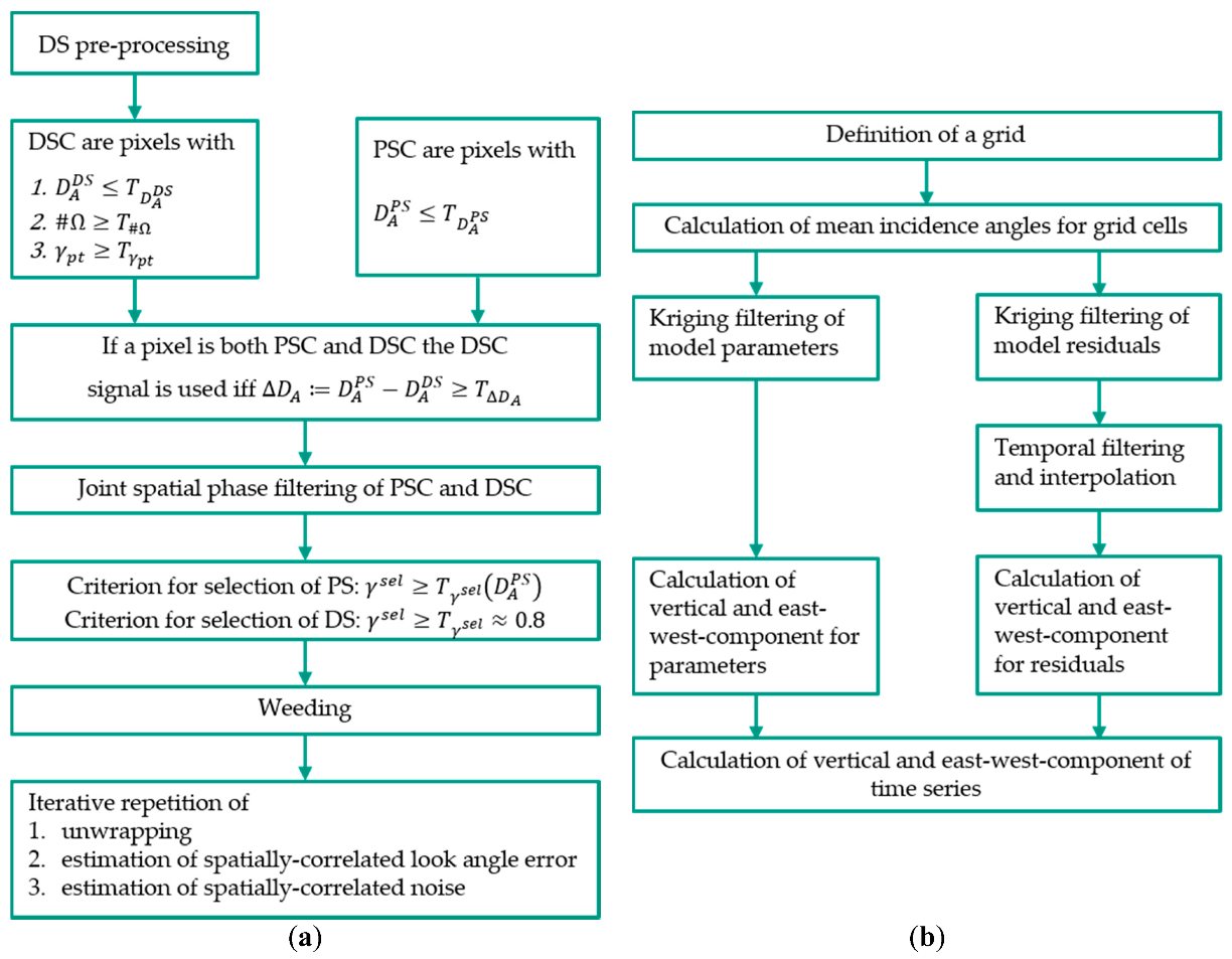
2.2.4. Orbit Combination

As DS and PS lie scattered and do not coincide for different orbits the two outputs of StaMPS have to be interpolated to common positions for the purpose of orbit combination. Likewise, times of acquisition do not agree, which makes temporal interpolation necessary. Unfortunately, interpolation and filtering tend to attenuate the estimated signal, particularly in the presence of noise. In this situation, the a priori knowledge about the deformation process that is reflected in the Multi-Mogi model described in Section 2.2.2 might potentially be used to preserve better the underlying signal. Hence orbit combination was implemented in two ways that are explained in the sequel. Before doing so, the principal steps of orbit combination are described:

• Definition of a grid to which values shall be interpolated (Gauß-Krüger coordinates and cells of 100 m times 100 m were used). As it makes sense to process only grid cells that contain points from both orbits their size has been chosen in a way that almost all points fall in such relevant grid cells.
• For each grid cell and both orbits a mean incidence angle was calculated by averaging over the values for the points lying in the cell.
• Kriging filtering [49] is used to interpolate for each acquisition and orbit the values of the displacement time series to the relevant grid cells.
• Time series of each orbit were filtered with robust quadratic regression in a moving window (of length 9 acquisitions) to remove any outliers left. Acquisitions outside the overlap of the two series were discarded. The period between 5 February 2015 and 21 December 2017 remained.
• The linear equation system for orbit combination for each point and using the interpolated time series was solved in an analogous way as was done by [50].

This basic version of orbit combination uses the displacement time series from StaMPS. In order to generate the results in the next section, a more complex approach has been adopted (Figure 4b gives a flowchart). A parametric linear model consisting of constant, linear trend, pressure response and seasonal movement was fitted to the displacement time series. This way they were split in a modeled part and an unmodeled residual. Steps 3 to 5 were modified accordingly: (a) for the unmodeled residual they have been performed as before; (b) for the modeled part kriging filtering has been applied to the parameters and the transformation from LOS to vertical and east-west component has been performed separately for them, which has the advantage to preserve the decomposition in the different components thus allowing to investigate them separately. The algorithm used for kriging filtering of the parameters is different for two of them. For all parameters the assumption of a constant drift is clearly not valid. Therefore, the use of ordinary kriging is not recommendable, while using universal kriging is a potential alternative. To apply universal kriging a model for the drift is required. We do not have one for all parameters. The first parameter is not relevant for displacement analysis and appears to represent not removed master atmosphere. Hence it does not need extra care and ordinary kriging has been applied. The second and third parameter are related to the geophysical behavior of the deposit. For these two parameters models for the drift have been constructed with help of the Multi-Mogi model and universal kriging has been performed. The fourth parameter has been filtered preliminary with ordinary kriging despite the named objection, as a model for the drift has not yet been devised. We will refer to this method as “geometric” for brevity.

Alternative to universal kriging filtering for the second and third parameter and transforming the result to vertical and horizontal coordinates a second approach was tested. For each of the two displacement parameters the parameters of the Multi-Mogi model were estimated by optimizing for both orbits at the same time the fit to the LOS displacement parameter values at their original, orbit dependent positions (cp. Section 2.2.1). In case of the linear component the value of $p_{lin}$ is determined that minimizes

$${\displaystyle \sum }_{\left(x,y\right)\in R^{asc}}{\left|p_{lin}^{asc}\left(x,y\right)-p_{lin}·A^{asc}\left(x,y\right)·{\displaystyle \sum }_{c\in C}{M}_c\left(x,y\right)\right|}^2+{\displaystyle \sum }_{\left(x,y\right)\in R^{desc}}{\left|p_{lin}^{desc}\left(x,y\right)-p_{lin}·A^{desc}\left(x,y\right)·{\displaystyle \sum }_{c\in C}{M}_c\left(x,y\right)\right|}^2$$

(12)

Here $R^{asc}$ and $R^{desc}$ are the sets of pixels from the two InSAR results for which the estimated model parameters $p_{lin}^{asc}\left(x,y\right)$ or $p_{lin}^{desc}\left(x,y\right)$ are bigger than some threshold. $A^{asc}\left(x,y\right)$ and $A^{desc}\left(x,y\right)$ are the vectors that project displacements according to the Multi-Mogi model to line of sight of each of the orbits. The value of $p_{pres}$ is determined analogously. With the obtained parameters of the Multi-Mogi model the displacement parameters in vertical and horizontal direction at arbitrary positions can be calculated. We will refer to this method as “Multi-Mogi”.

Furthermore, it has to be remarked that the procedure of estimating the parameters of the Multi-Mogi model differed for the two parameters. $p_{lin}$ describes the subsidence caused by convergence of the caverns. Therefore, all caverns contribute to the deformation, although not necessarily to the same degree. On the other hand, $p_{pres}$ describes the magnitude of the response to pressure changes in gas filled caverns. It is assumed that caverns filled with liquids do not contribute to this component of the displacement signal and consequentially these caverns are not included in the model in this case. Finally, points with big value of the parameter of the seasonal component have been masked out in order to prevent any adverse effects on the estimation because of correlation of the model for pressure induced displacement with the seasonal model.

3. Results

Data from both orbits have been processed with DS-preprocessing and the augmented StaMPS algorithm. A four dimensional linear phase model has been fitted to each time series of the results.

3.1. Joint Processing of DS and PS

Figure 5 displays the model parameters estimated for both orbits. On the left hand side results from ascending orbit are shown and on the right hand side those of descending orbit. From top to bottom linear trend, pressure response and seasonal signal are given. The color code for the linear trend expresses mm/y and negative values indicate subsidence. For the other two parameters the maximal displacement in mm is depicted, i.e., the difference between maximum and minimum of the signal. Significant linear trends can be observed over the whole cavern field. Apparently all caverns suffer from convergence and contribute to the signal. The other two components of the displacement signal express differently in the western part and in the eastern part. In the western part, the majority of liquid filled caverns is situated and a fen can be found that is displayed by a brownish color in the background map (cp. Figure 1). In the eastern part, gas filled caverns dominate (cp. Figure 1). As one would expect, surface movements modeled by the pressure response occur over the eastern part of the cavern field, where gas is stored. Seasonal movements, on the other hand, are restricted to a fen in the western part of the cavern field. We demonstrate below that the seasonal movements are presumably caused by groundwater level changes. The presence of horizontal movements can be recognized for linear trends and, less distinctly, for displacements with pressure changes, e.g., the areas of strongest displacement appear to be different. The points with significant seasonal signal in the fen are all DS and no information was available in this area from a reference result generated with StaMPS using only PS. It is noteworthy that these points extend the usable information on convergence and pressure response to this area (cp. also Figures 12 and 13). The related case of using InSAR to determine displacements of pasture on drained peat soils was demonstrated to be a challenging task [51,52], but the authors predicted that the 6-day repeat pass of Sentinel-1 might improve the situation. The use of Sentinel-1 and the presence of structures caused by peat cutting might have contributed to a successful evaluation of the DS signals in this work. Figure 6 displays as indicator of pixel quality the root mean square (RMS) of the residual phases for each point for both orbits. Residual phase means here phase of the final result minus modelled phase. The residual phase comprises non-compensated errors (e.g., white noise) and the not modelled signal. The latter presumably gives a partial explanation for the high values of RMS over the fen, because the actual highly irregular seasonal signal supposedly deviates from its model.

Figure 7 displays two time series of levels of groundwater measurements (GWM) taken in the fen area together with the mean detrended displacement signals of nearby DS of both orbits (the InSAR signals have been scaled to match the groundwater levels). A good correlation between groundwater levels and surface movements detected by InSAR is evident. However, a small time delay between InSAR and GWM is visible that might be explained by the time the water needs to seep to the location of GWM after rain.

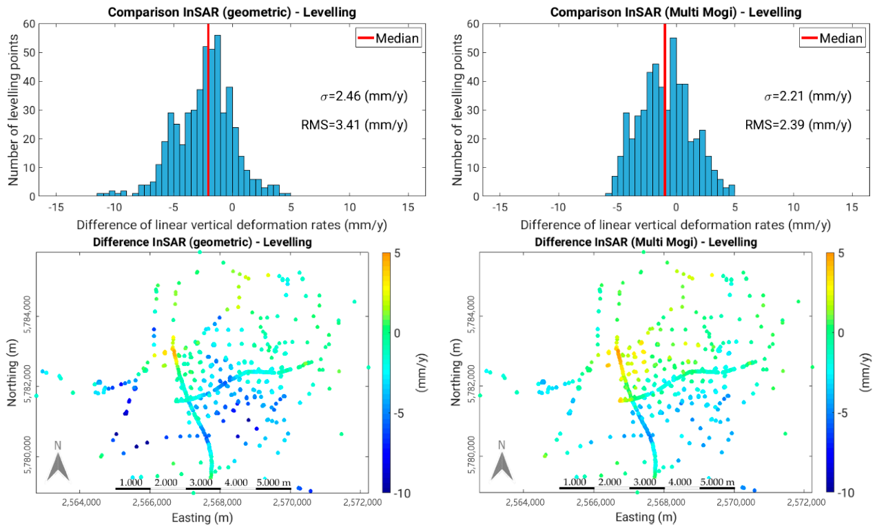
3.2. Orbit Combination

In this section results obtained after orbit combination are presented. As explained in Section 2.2.4 orbit combination was performed by two different methods to which is referred as geometric or Multi-Mogi in the following. In order to assess the quality of the different approaches orbit combinations have been done at those coordinates, where levelling data are available. This is different from the purpose of obtaining displacement fields as presented below, where the combination is done for those cells of a raster that contains information from both orbits. As a characteristic of quality the standard deviation σ between InSAR time series and levelling has been calculated at each coordinate. To do so, some assumptions were made. Levelling measurements were performed each year between middle of May and middle of July. It is not possible to assign a precise point of time to measurements. Hence σ was calculated by interpolating the InSAR displacement time series to the 15th of June of each year. Furthermore, data from some of the levelling locations were not used. These either comprise only two values or are not consistent with nearby measurements. For the latter a comparison with InSAR results does not make sense as this requires interpolation to the positions of the levelling points and cannot capture local peculiarities. This way 517 of 548 levelling points were retained and used for the comparison. Figure 8 shows the color coded values of σ for the two investigated approaches. The results on the left-hand side use geometric orbit combination, those on the right-hand side the Multi-Mogi approach. Both comparisons show deviations between InSAR result and levelling at two regions, where the approximately north-south running levelling line leaves the subsidence bowl. Deviations for those using the Multi-Mogi approach are less severe. Two points with large deviation between the geometric approach and levelling stand out, while Multi-Mogi is not sensitive to estimation errors affecting single points by design and provides good results. This is confirmed by the histograms of differences between InSAR and levelling in Figure 9. The distinct negative bias observed for the geometric approach is a bit surprising as it means that the deformation measured by InSAR is stronger than that measured by levelling. Partially, it can be explained by the spatial arrangement of PS and Ds on the one hand and levelling points on the other. The larger portion of the points showing significant differences are situated along the road south of the cavern field. North of the road is the area of strongest subsidence, which is well covered by InSAR, while south of the road an area without InSAR points abuts. Hence, kriging uses predominately points with subsidence rates higher than measured by levelling to interpolate InSAR results to levelling positions. Another source of error is the ignorance of the north component of displacement for the geometric approach. To get an idea of the order of its consequences this error has been calculated based on the north component estimated with Multi-Mogi (Figure 10). It has 0.08 mm/y bias and 1.3 mm/y standard deviation. From this it appears that it does not significantly influence the bias and merely increases the standard deviation notably.

Figure 11 shows the vertical displacement for some time series for each of the approaches together with the model curves estimated and levelling. The model curves are a combination of three components: linear subsidence, pressure induced and seasonal displacement. The given value of σ is calculated for Multi-Mogi and is intended to convey a visual impression of the significance of the deviation that goes along with the value of σ. Figure 11d is an example where the non-modeled signal contains valuable information at locations, where the model does not fit perfectly to the time series.

There are also cases where a larger deviation possibly is due to inaccuracies of levelling. Figure 11e shows a suspected case.

Figure 12 shows the linear vertical displacement rate estimated from the time series generated with the Multi-Mogi approach, where data have been interpolated to a raster. Linear rates for levelling points are displayed as crosses in the same color scale. Both data sets blend nicely, what demonstrates again the good agreement between results from Multi-Mogi and levelling measurements. It is clearly seen that the DS located at the fen carry relevant information about the convergence process of the caverns and thereby contribute to a spatially dense displacement field that could not have been obtained from PS alone. However, Multi-Mogi does not capture as well the horizontal displacement field as it does the vertical as indicates a comparison with the geometric approach. The first row of Figure 13 shows linear displacement rates in vertical and east-west direction estimated from the time series generated with geometric orbit combination. The second row shows the corresponding results generated with the Multi-Mogi approach. The horizontal displacement extends far into the surroundings of the deposit and appears blurred in comparison with the result of the geometric combination.

Finally, Figure 14 displays for geometric orbit combination the vertical and east-west component of the parameters for the pressure response and the seasonal signal. The pressure signal which is related to deeply situated sources, has a large spatial dimension in both components. In contrast to this, the seasonal effect is restricted to the vertical component in the immediate vicinity of the fen, which indicates that the water-driven deformation takes place only in the uppermost soil layers.

4. Discussion

The results presented in Section 3 demonstrate that multi-temporal InSAR techniques using Sentinel-1 data allow obtaining valuable information about complex surface displacement fields as that of the underground storage at Epe. The InSAR derived displacements are in reasonable agreement with levelling data for geometric orbit combination and in good agreement for the Multi-Mogi approach. They complement levelling with information from additional locations and deliver horizontal movements. In particular, a high temporal sampling is possible that is difficult to achieve with levelling. The successful analysis has been made possible by combining StaMPS with DS pre-processing and introducing a displacement model that improved unwrapping as well as orbit combination. DS allow to extract information also in areas, where no PS are available, in particular over the fen in the western part of the cavern field. In this way a more complete description of the displacement field is obtained.

The displacement model, in addition to its benefits for processing, helps in interpreting the observations by decomposing the displacement signal in physically founded constituents. Although direct access to absolute pressure data from each cavern was not given, the high correlations of InSAR time series with the modeled pressure response based on filling levels of AGSI as a pressure surrogate and on assuming propagation through a visco-elastic medium, suggests that the proposed causal relationship exists and operational pressure changes in the caverns are accompanied by surface displacements of up to ± 6 mm. The presented model driven approach facilitates a clear separation of the pressure related displacements from ground water induced surface movements.

The InSAR based results also exhibit some shortcomings. The results of the geometric approach for the vertical and east-west component of displacement suffer from ignorance of the north-south component but still are reasonable. The observed bias between InSAR and levelling can be explained partially by the required interpolation. On the other hand, the Multi-Mogi approach captures vertical displacement well. However, it does overestimate the magnitude of horizontal displacement. This shortcoming presumably can be accounted for by the following two arguments:

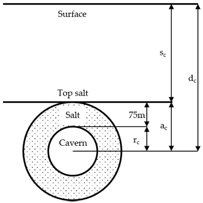
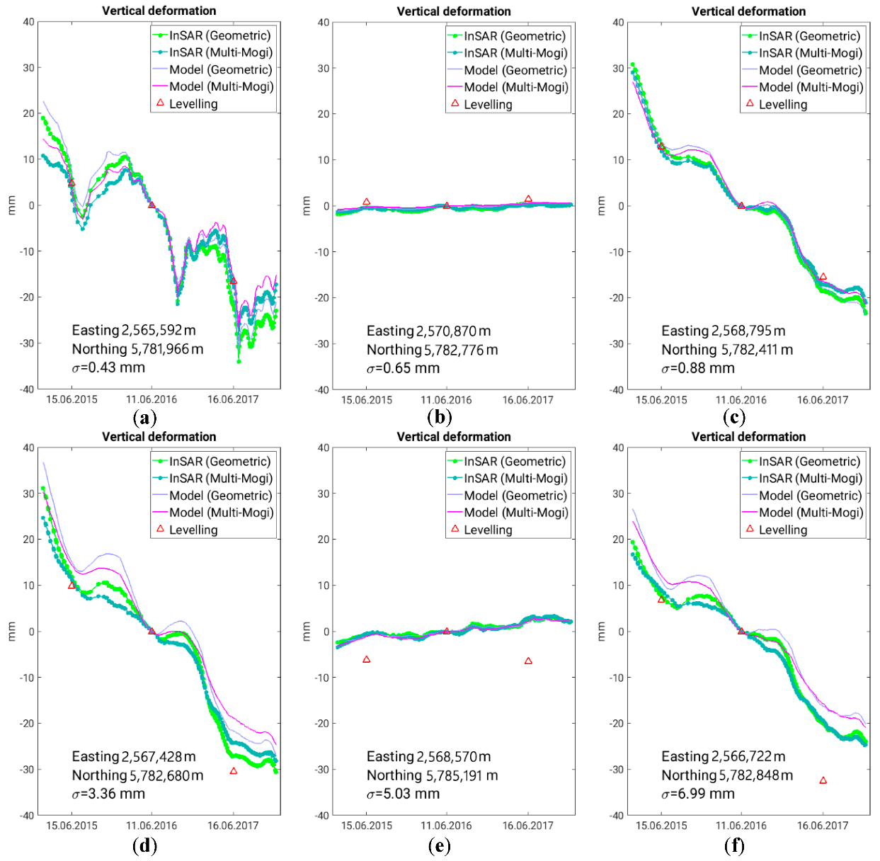
• As already discussed above, the geophysical situation is simplistically modelled. In particular, the model assumes that the caverns each are in the center of a salt sphere while in reality the salt is deposited as an approximately horizontal layer. We also deliberated if the elongated shape of the caverns in vertical direction might cause a bigger ratio between magnitude of vertical and horizontal displacement than is predicted by the Mogi model, but because of their depth of more than 1000 m this likely has no influence.
• The values of the incidence angles may at least partially explain that the Multi-Mogi estimation is less influenced by horizontal displacement and performs better for vertical displacement.

Future research might help to resolve these shortcomings. A better modeling of the geophysical realities potentially can provide good estimation of vertical as well as of horizontal displacement. Finally, repeating this study with data from a longer period would serve to validate the approach presented here.

5. Conclusions

In this study the complex displacement field over the cavern storage site at Epe, NW-Germany, was investigated. The temporal behavior of each point could be modeled as linear combination of three components: linear subsidence caused by cavern convergence, displacement responding to pressure changes in the gas filled caverns and a seasonal movement over a fen that shows a good correlation with groundwater measurements. In order to achieve the presented results, simplistic geomechanical modelling of the temporal signal, improvements of InSAR processing and component-wise orbit combination were introduced.

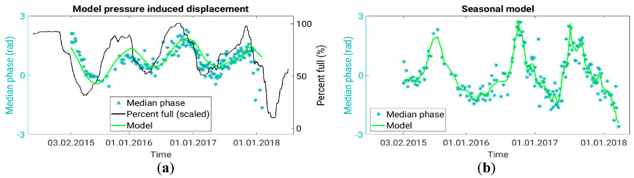
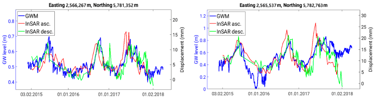
• Geomechanical modelling provided the temporal model for displacements responding to pressure changes in the gas filled caverns. While for reservoirs in elastic media the displacements are directly proportional to pressure changes of the gas, pressure signals passing through a viscos medium (salt) experience a retardation that can be described by equation (2). The presented approach is to the best of our knowledge the first, where such a model is derived for the use with InSAR for caverns situated in salt.
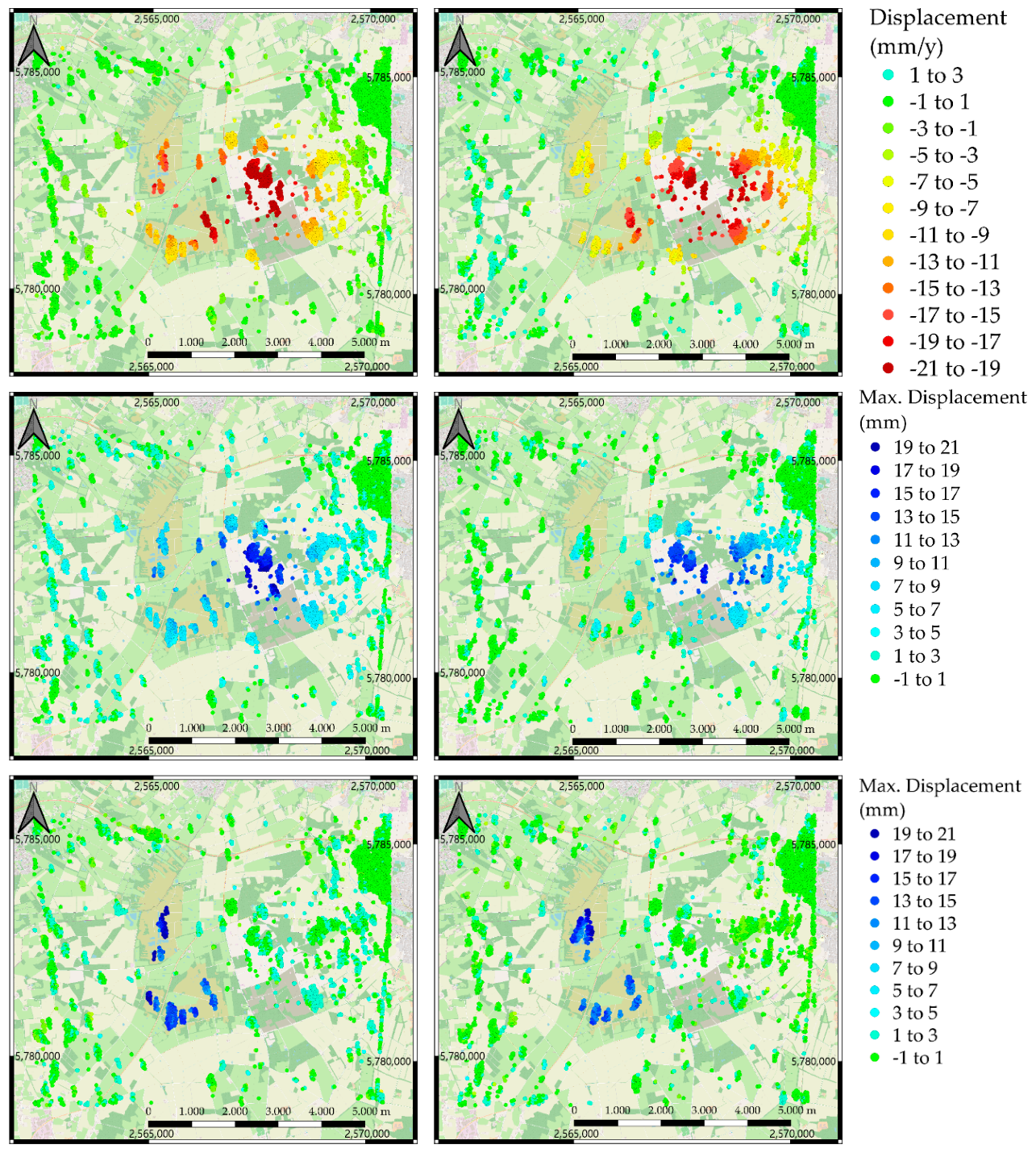
• StaMPS needed to be improved in several ways for dealing with the challenging displacement field at Epe. The possibility to use a phase model was implemented in order to support unwrapping and to enhance signal filtering. Furthermore, the iterative estimation scheme of StaMPS was refined, what prevents leakage of the displacement signal to the spatially correlated noise term. In addition, joint processing of PS and DS as recently introduced in [20] was applied. The results presented in this study confirm the validity of the approach of [20]. In particular, the DS allowed to extend observations to the fen in the western part of the storage site, where no information was available with PS alone.
• A novelty of the orbit combination implemented for this study is that the different components of the phase model are combined separately. This allowed for a better understanding of the phenomena that contribute to the displacement field. We named this approach geometric orbit combination.

In addition, a method that allows to perform an orbit combination based on simplistic geomechanical modelling of the spatial displacement field was presented. It treats caverns as Mogi sources, whose volume changes because of convergence lead to linear subsidence and whose pressure changes result in the pressure induced displacement. The model assumes for each of these two components one unknown parameter that is estimated such that the projections to line of sight for both orbits optimally approximate the orbit-wise estimations. We named this approach Multi Mogi approach.

The vertical components of the estimated displacements were validated with data from 517 levelling points available over the storage site. The agreement of linear trends of vertical displacement from geometric orbit combination and levelling was reasonable (root mean square 3.41 mm/y). The agreement of linear trends of vertical displacement from the Multi Mogi approach and levelling was very good (root mean square 2.39 mm/y). Unfortunately, the Multi Mogi approach overestimated the east-west component of displacement. This may be due to insufficient knowledge of physical parameters or imperfections of the model itself and deserves further investigation.

References

1. Vasco, D.W.; Ferretti, A.; Novali, F. Estimating permeability from quasi-static deformation: Temporal variations and arrival-time inversion. Geophysics 2008, 73, O37–O52. [Google Scholar] [CrossRef] [Green Version]
2. Vasco, D.W.; Ferretti, A.; Novali, F. Reservoir monitoring and characterization using satellite geodetic data: Interferometric synthetic aperture radar observations from the Krechba field, Algeria. Geophysics 2008, 73, WA113–WA122. [Google Scholar] [CrossRef]
3. Vasco, D.W.; Rucci, A.; Ferretti, A.; Novali, F.; Bissell, R.C.; Ringrose, P.S.; Mathieson, A.S.; Wright, I.W. Satellite-based measurements of surface deformation reveal fluid flow associated with the geological storage of carbon dioxide. Geophys. Res. Lett. 2010, 37, 1–5. [Google Scholar] [CrossRef] [Green Version]
4. Tamburini, A.; Bianchi, M.; Giannico, C.; Novali, F. Retrieving surface deformation by PSInSARTM technology: A powerful tool in reservoir monitoring. Int. J. Greenh. Gas Control 2010, 4, 928–937. [Google Scholar] [CrossRef]
5. Rucci, A.; Vasco, D.W.; Novali, F. Fluid pressure arrival time tomography: Estimation and assessment in the presence of inequality constraints, with an application to production at the Krechba field, Algeria. Geophysics 2010, 75, 39–55. [Google Scholar] [CrossRef]
6. Rocca, F.; Rucci, A.; Ferretti, A.; Bohane, A. Advanced InSAR interferometry for reservoir monitoring. First Break 2013, 31, 77–85. [Google Scholar]
7. Rucci, A.; Vasco, D.W.; Novali, F. Monitoring the geologic storage of carbon dioxide using multicomponent SAR interferometry. Geophys. J. Int. 2013, 193, 197–208. [Google Scholar] [CrossRef] [Green Version]
8. Teatini, P.; Castelletto, N.; Ferronato, M.; Gambolati, G.; Janna, C.; Cairo, E.; Marzorati, D.; Colombo, D.; Ferretti, A.; Bagliani, A.; et al. Geomechanical response to seasonal gas storage in depleted reservoirs: A case study in the Po River basin, Italy. J. Geophys. Res. Space Phys. 2011, 116. [Google Scholar] [CrossRef]
9. Fokker, P.A.; Visser, K.; Peters, E.; Kunakbayeva, G.; Muntendam-Bos, A. Inversion of surface subsidence data to quantify reservoir compartmentalization: A field study. J. Pet. Sci. Eng. 2012, 10–21. [Google Scholar] [CrossRef]
10. Comola, F.; Janna, C.; Lovison, A.; Minini, M.; Tamburini, A.; Teatini, P. Efficient global optimization of reservoir geomechanical parameters based on synthetic aperture radar-derived ground displacements. Geophysics 2016, 81, M23–M33. [Google Scholar] [CrossRef] [Green Version]
11. Velasco, V.; Sanchez, C.; Papoutsis, I.; Antoniadi, S.; Kontoes, C.; Aifantopoulou, D.; Paralykidis, S. Ground deformation mapping and monitoring of salt mines using InSAR technology. In Proceedings of the Solution Mining Research Institute Fall 2017 Technical Conference, Münster, Germany, 25–26 September 2017. [Google Scholar]
12. Burnol, A.; Aochi, H.; Raucoules, D.; Veloso, F.M.L.; Koudogbo, F.N.; Fumagalli, A.; Chiquet, P.; Maisons, C. Wavelet-based analysis of ground deformation coupling satellite acquisitions (Sentinel-1, SMOS) and data from shallow and deep wells in Southwestern France. Sci. Rep. 2019, 9, 1–12. [Google Scholar] [CrossRef] [Green Version]
13. Ferretti, A.; Tamburini, A.; Novali, F.; Fumagalli, A.; Falorni, G.; Rucci, A. Impact of high resolution radar imagery on reservoir monitoring. Energy Procedia 2011, 4, 3465–3471. [Google Scholar] [CrossRef] [Green Version]
14. Kuehn, F.; Hoth, P.; Stark, M.; Burren, R.; Hole, J. Experience with satellite radar for gas storage monitoring. Erdöl Erdgas Kohle 2009, 125, 452–460. [Google Scholar]
15. Jha, B.; Bottazzi, F.; Wojcik, R.; Coccia, M.; Bechor, N.; McLaughlin, D.; Herring, T.; Hager, B.H.; Mantica, S.; Juanes, R. Reservoir characterization in an underground gas storage field using joint inversion of flow and geodetic data. Int. J. Numer. Anal. Methods Géoméch. 2015, 39, 1619–1638. [Google Scholar] [CrossRef] [Green Version]
16. Morgan, J.; Snider-Lord, A.C.; Ambs, D.C. InSAR for monitoring cavern integrity: 2D surface movement over Bryan Mound. In Proceedings of the Solution Mining Research Institute Spring 2018 Technical Conference, Salt Lake City, UT, USA, 18 June 2018. [Google Scholar]
17. Meyers, M.A.; Chawla, K.K. Mechanical Behavior of Materials, 2nd ed.; Cambridge University Press: New York, NY, USA, 2009; pp. 1–856. [Google Scholar]
18. Ferretti, A.; Fumagalli, A.; Novali, F.; Prati, C.; Rocca, F.; Rucci, A. A new algorithm for processing interferometric data-stacks: SqueeSAR. IEEE Trans. Geosci. Remote Sens. 2011, 49, 3460–3470. [Google Scholar] [CrossRef]
19. Even, M.; Schulz, K. InSAR deformation analysis with distributed scatterers: A review complemented by new advances. Remote Sens. 2018, 10, 744. [Google Scholar] [CrossRef] [Green Version]
20. Even, M. Adapting stamps for jointly processing distributed scatterers and persistent scatterers. In Proceedings of the IGARSS 2019–2019 IEEE International Geoscience and Remote Sensing Symposium, Yokohama, Japan, 28 July–2 August 2019; pp. 2046–2049. [Google Scholar] [CrossRef]
21. Hooper, A.; Segall, P.; Zebker, H. Persistent scatterer interferometric synthetic aperture radar for crustal deformation analysis, with application to Volcán Alcedo, Galápagos. J. Geophys. Res. Space Phys. 2007, 112, 1–21. [Google Scholar] [CrossRef] [Green Version]
22. StaMPS Homepage. Available online: https://homepages.see.leeds.ac.uk/~earahoo/stamps/ (accessed on 12 September 2013).
23. Gray, L. Using multiple RADARSAT InSAR pairs to estimate a full three-dimensional solution for glacial ice movement. Geophys. Res. Lett. 2011, 38, 1–6. [Google Scholar] [CrossRef]
24. Hu, J.; Li, Z.; Ding, X.; Zhu, J.; Zhang, L.; Sun, Q. Resolving three-dimensional surface displacements from InSAR measurements: A review. Earth Sci. Rev. 2014, 133, 1–17. [Google Scholar] [CrossRef]
25. Joughin, I.; Kwok, R.; Fahnestock, M. Interferometric estimation of three-dimensional ice-flow using ascending and descending passes. IEEE Trans. Geosci. Remote Sens. 1998, 36, 25–37. [Google Scholar] [CrossRef] [Green Version]
26. Mohr, J.J.; Reeh, N.; Madsen, S.N. Three-dimensional glacial flow and surface elevation measured with radar interferometry. Nature 1998, 391, 273–276. [Google Scholar] [CrossRef]
27. Cascini, L.; Fornaro, G.; Peduto, D. Advanced low and full-resolution DInSAR map generation for slow-moving landslide analysis at different scales. Eng. Geol. 2010, 112, 29–42. [Google Scholar] [CrossRef]
28. Bos, A.G.; Usai, S.; Spakman, W. A joint analysis of GPS motions and InSAR to infer the coseismic surface deformation of the Izmit, Turkey earthquake. Geophys. J. Int. 2004, 158, 849–863. [Google Scholar] [CrossRef] [Green Version]
29. Fuhrmann, T.; Cuenca, M.C.; Knöpfler, A.; Van Leijen, F.; Mayer, M.; Westerhaus, M.; Hanssen, R.; Heck, B. Estimation of small surface displacements in the Upper Rhine Graben area from a combined analysis of PS-InSAR, levelling and GNSS data. Geophys. J. Int. 2015, 203, 614–631. [Google Scholar] [CrossRef] [Green Version]
30. Michel, R.; Avouac, J.-P.; Taboury, J.; Michel, R. Measuring ground displacements from SAR amplitude images: Application to the Landers Earthquake. Geophys. Res. Lett. 1999, 26, 875–878. [Google Scholar] [CrossRef] [Green Version]
31. Michel, R.; Avouac, J.-P.; Taboury, J. Measuring near field coseismic displacements from SAR images: Application to the Landers Earthquake. Geophys. Res. Lett. 1999, 26, 3017–3020. [Google Scholar] [CrossRef] [Green Version]
32. Bechor, N.B.D.; Zebker, H.A. Measuring two-dimensional movements using a single InSAR pair. Geophys. Res. Lett. 2006, 33, 1–5. [Google Scholar] [CrossRef] [Green Version]
33. Samiei-Esfahany, S.; Hanssen, R.; van Thienen-Visser, K.; Muntendam-Bos, A. On the effect of horizontal deformation on InSAR subsidence estimates. In Proceedings of the Fringe Workshop, ESRIN, Frascati, Italy, 30 November–4 December 2009. [Google Scholar]
34. Wright, T.J.; Parsons, B.E.; Lu, Z. Toward mapping surface deformation in three dimensions using InSAR. Geophys. Res. Lett. 2004, 31, 1–5. [Google Scholar] [CrossRef] [Green Version]
35. Manzo, M.; Ricciardi, G.; Casu, F.; Ventura, G.; Zeni, G.; Borgström, S.; Berardino, P.; Del Gaudio, C.; Lanari, R. Surface deformation analysis in the Ischia Island (Italy) based on spaceborne radar interferometry. J. Volcanol. Geotherm. Res. 2006, 151, 399–416. [Google Scholar] [CrossRef]
36. Fuhrmann, T.; Garthwaite, M.C. Resolving three-dimensional surface motion with InSAR: Constraints from multi-geometry data fusion. Remote Sens. 2019, 11, 241. [Google Scholar] [CrossRef] [Green Version]
37. Mogi, K. Relations between the eruptions of various volcanoes and the deformations of the ground surfaces around them. Earthq. Res. Inst. 1958, 36, 99–134. [Google Scholar]
38. Aggregated Gas Storage Inventory (AGSI). Available online: https://agsi.gie.eu/#/ (accessed on 5 December 2019).
39. Liu, W.; Völkner, E.; Minkley, W.; Popp, T. F+E Endlagerung: Zusammenstellung der Materialparameter für THM-Modellberechnungen, Ergebnisse aus dem Vorhaben KOSINA; Bundesanstalt für Geowissenschaften und Rohstoffe: Hannover, Germany, 2017. [Google Scholar]
40. Shamshiri, R.; Nahavandchi, H.; Motagh, M.; Hooper, A. Efficient ground surface displacement monitoring using sentinel-1 data: Integrating Distributed Scatterers (DS) identified using two-sample t-test with Persistent Scatterers (PS). Remote Sens. 2018, 10, 794. [Google Scholar] [CrossRef] [Green Version]
41. Pepe, A.; Yang, Y.; Manzo, M.; Lanari, R. Improved EMCF-SBAS processing chain based on advanced techniques for the noise-filtering and selection of small baseline multi-look DInSAR Interferograms. IEEE Trans. Geosci. Remote Sens. 2015, 53, 4394–4417. [Google Scholar] [CrossRef]
42. Wang, Y.; Zhu, X.X. Robust estimators for multipass SAR interferometry. IEEE Trans. Geosci. Remote Sens. 2015, 54, 968–980. [Google Scholar] [CrossRef]
43. Samiei-Esfahany, S.; Martins, J.E.; Van Leijen, F.; Hanssen, R.F. Phase estimation for distributed scatterers in InSAR stacks using integer least squares estimation. IEEE Trans. Geosci. Remote Sens. 2016, 54, 5671–5687. [Google Scholar] [CrossRef] [Green Version]
44. Lin, K.-F.; Perissin, D. Identification of statistically homogeneous pixels based on one-sample test. Remote Sens. 2017, 9, 37. [Google Scholar] [CrossRef] [Green Version]
45. Verde, S.; Reale, D.; Pauciullo, A.; Fornaro, G. Improved small baseline processing by means of CAESAR eigen-interferograms decomposition. ISPRS J. Photogramm. Remote Sens. 2018, 139, 1–13. [Google Scholar] [CrossRef]
46. Ansari, H.; De Zan, F.; Bamler, R. Efficient phase estimation for interferogram stacks. IEEE Trans. Geosci. Remote Sens. 2018, 56, 4109–4125. [Google Scholar] [CrossRef]
47. Ferretti, A.; Fumagalli, A.; Novali, F.; De Zan, F.; Rucci, A.; Tebaldini, S. Process for Filtering Interferograms Obtained from SAR Images Acquired on the Same Area. CA Patent Application 2,767,144, 13 January 2011. [Google Scholar]
48. Guarnieri, A.M.; Tebaldini, S. On the exploitation of target statistics for SAR interferometry applications. IEEE Trans. Geosci. Remote Sens. 2008, 46, 3436–3443. [Google Scholar] [CrossRef]
49. Wackernagel, H. Multivariate Geostatistics, 3rd ed.; Springer: Berlin/Heidelberg, Germany, 2003; pp. 1–387. [Google Scholar]
50. Samsonov, S.V.; D’Oreye, N. Multidimensional Small Baseline Subset (MSBAS) for two-dimensional deformation analysis: Case study Mexico City. Can. J. Remote Sens. 2017, 43, 318–329. [Google Scholar] [CrossRef]
51. Morishita, Y.; Hanssen, R.F. Temporal decorrelation in L-, C-, and X-band satellite radar interferometry for pasture on drained peat soils. IEEE Trans. Geosci. Remote Sens. 2014, 53, 1096–1104. [Google Scholar] [CrossRef]
52. Morishita, Y.; Hanssen, R.F. Deformation parameter estimation in low coherence areas using a multisatellite InSAR approach. IEEE Trans. Geosci. Remote Sens. 2015, 53, 4275–4283. [Google Scholar] [CrossRef]
Publisher’s Note: MDPI stays neutral with regard to jurisdictional claims in published maps and institutional affiliations.
Figure 1. Locations of levelling measurements (markers colored according to linear trends), ground water measurements (GWM) with daily logging and of caverns. The background map is from Open Street Map.
Remotesensing 12 03348 g001
Figure 2. (a) Model for pressure response with combination of median time series of both orbits selected from preliminary InSAR results and average filling level f c a v e r n as in equation (10); (b) Model for seasonal displacement together with combination of median time series of both orbits selected from preliminary InSAR results.
Remotesensing 12 03348 g002
Figure 3. Sketch of the geometric arrangement of a cavern as used for modelling ( d c depth of cavern center, s c top salt, a c radius of salt sphere, r c cavern radius).
Remotesensing 12 03348 g003
Figure 4. Flowcharts for joint processing of PS and DS and for orbit combination. Symbols are explained in the text.
Remotesensing 12 03348 g004
Figure 5. Estimated parameters in line of sight. On the left from ascending orbit, on the right from descending orbit. From first row to third row: linear rate, pressure response, seasonal displacement. The brownish color surrounding the points with strongest seasonal displacement displays the fen.
Remotesensing 12 03348 g005
Figure 6. Root Mean Square (RMS) of residual phase. Left-hand side from ascending orbit, right-hand side from descending orbit.
Remotesensing 12 03348 g006
Figure 7. Examples of ground water levels together with scaled mean over InSAR time series of nearby points from each orbit.
Remotesensing 12 03348 g007
Figure 8. Standard deviations of differences between InSAR results and levelling. Left-hand side from geometric orbit combination, right-hand side Multi-Mogi approach.
Remotesensing 12 03348 g008
Figure 9. Histograms and scatter plots of differences between InSAR results and levelling. Left-hand side from geometric orbit combination, right-hand side Multi-Mogi approach.
Remotesensing 12 03348 g009
Figure 10. Error of vertical displacement because of ignorance of north-south component.
Remotesensing 12 03348 g010
Figure 11. Examples of vertical displacement time series for selected points.
Remotesensing 12 03348 g011
Figure 12. Linear displacement rate transformed to vertical with Multi-Mogi approach (bullets) together with linear rates from levelling (crosses).
Remotesensing 12 03348 g012
Figure 13. Linear displacement rates transformed to vertical and east-west direction. First row from geometric orbit combination, second row with Multi-Mogi approach.
Remotesensing 12 03348 g013
Figure 14. Parameters for pressure response and seasonal displacement transformed to vertical and east-west direction from geometric orbit combination.
Remotesensing 12 03348 g014