Use of Remotely Sensed Data to Enhance Estimation of Aboveground Biomass for the Dry Afromontane Forest in South-Central Ethiopia

 , , , ,
Abstract
1. Introduction
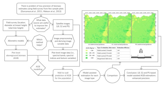
2. Materials and Methods
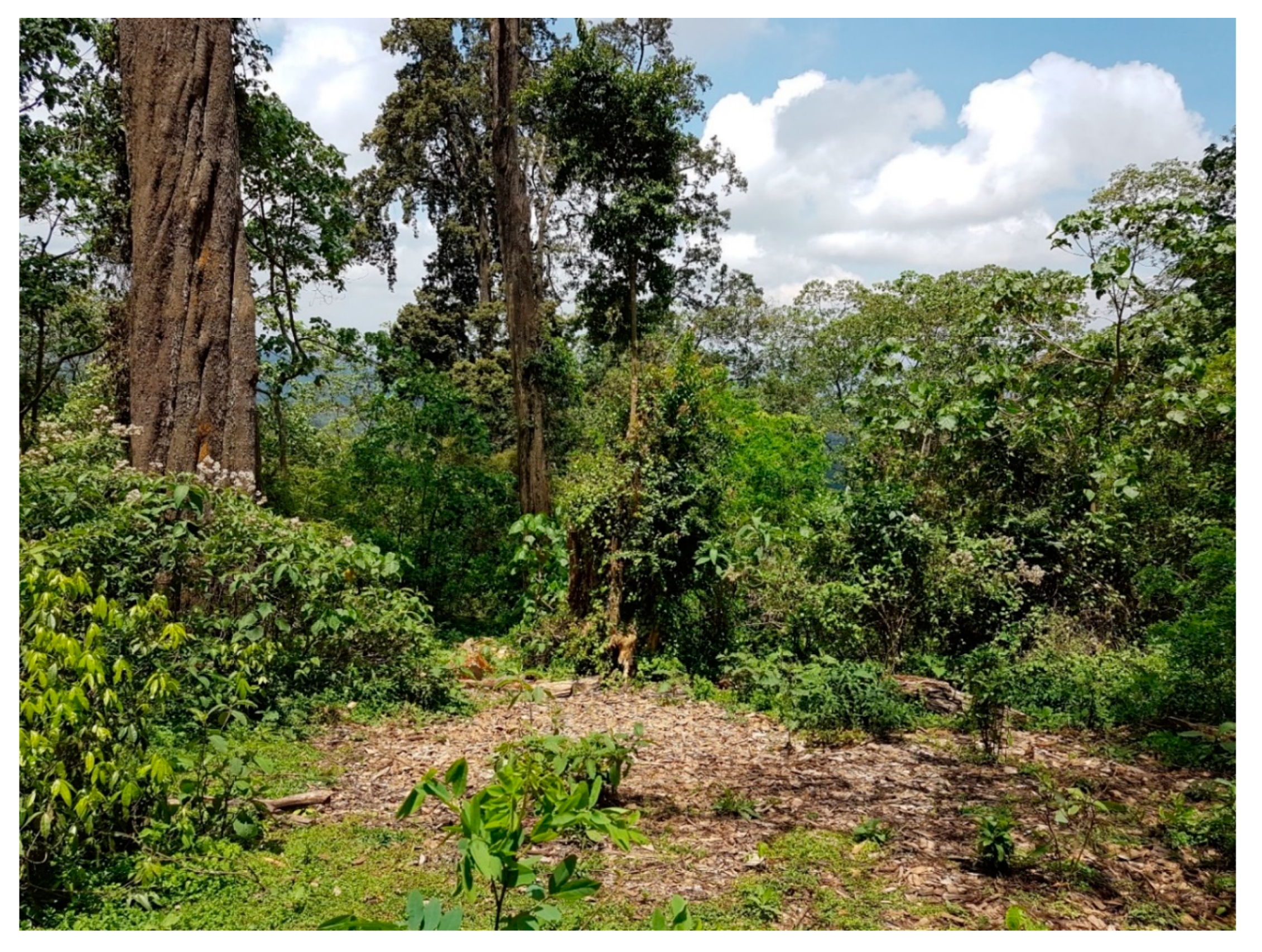
2.1. Description of the Study Area
2.2. Field Data Collection
2.3. Plot-Level AGB Estimation
2.4. Satellite Image Acquisition
2.5. Image Processing and Independent Variable Definition
2.6. Variable Selection and Model Fitting
2.7. Model Validation
2.8. Population-Level Estimation and Efficiency Assessment
3. Results
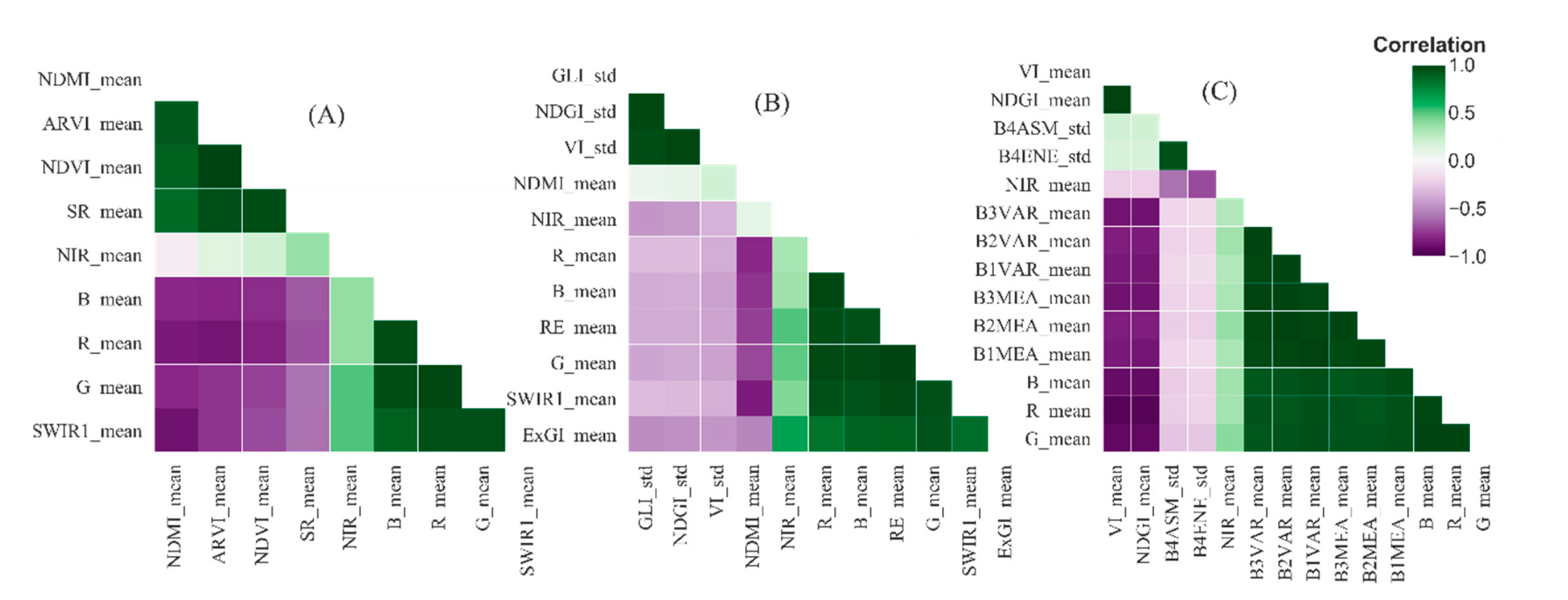
3.1. Relationship of Independent Variables with AGB
3.2. Variable Selection for the Prediction Models
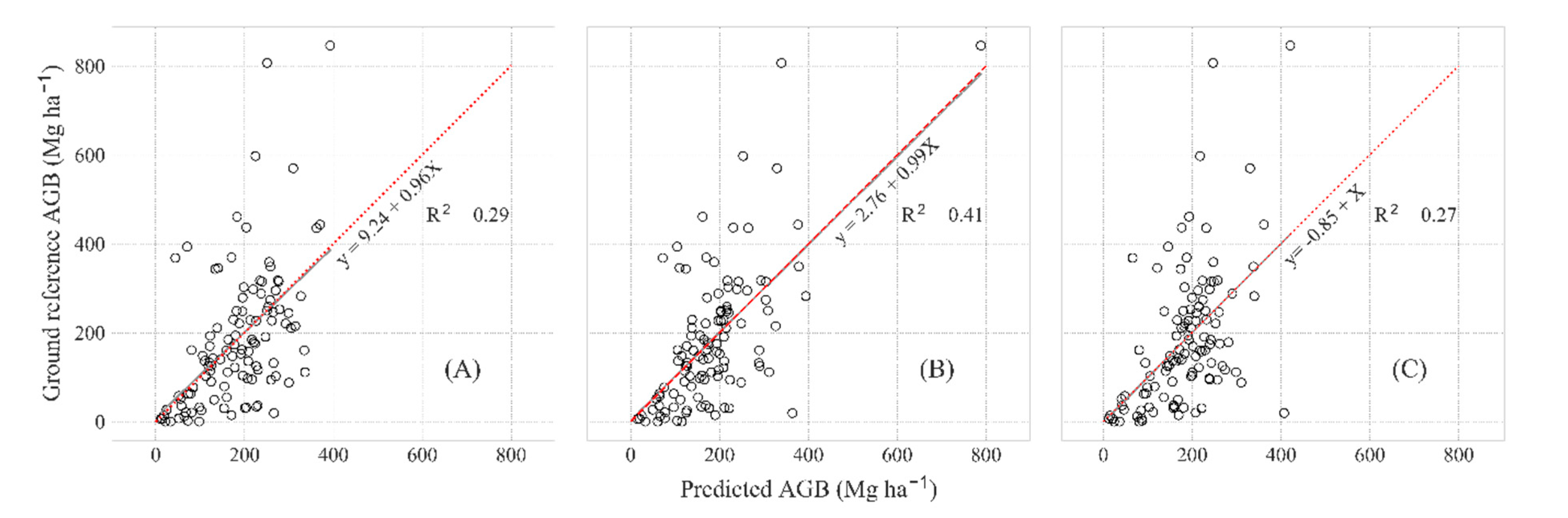
3.3. Selected AGB Models for Each Image Type
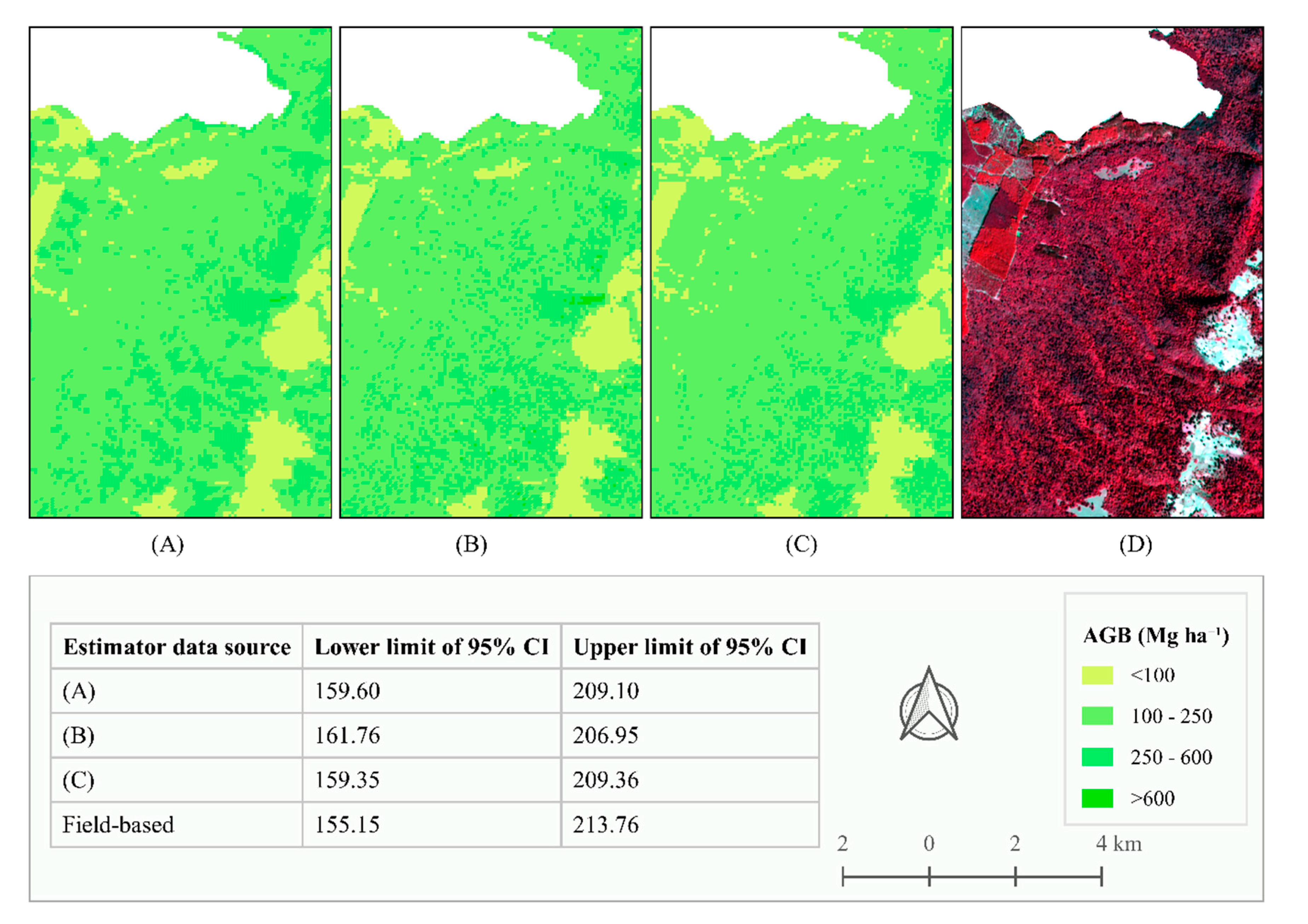
3.4. Estimation and Mapping of AGB Using the Selected Models
4. Discussion
4.1. Variable Exploration for Estimating AGB and Model Selection
4.2. Model Characteristics and Their Contribution to Enhance AGB Estimation
5. Conclusions
Author Contributions
Funding
Acknowledgments
Conflicts of Interest
References
- Bonan, G.B. Forests and climate change: Forcings, feedbacks, and the climate benefits of forests. Science 2008, 320, 1444–1449. [Google Scholar] [CrossRef] [PubMed]
- Anderson, J.W. The Kyoto Protocol on Climate Change; Resources for the Future: Washington, DC, USA, 1998; pp. 1–21. Available online: https://media.rff.org/documents/RFF-RPT-kyotoprot.pdf (accessed on 17 September 2019).
- UNFCCC. Decisions adopted by the Conference of the Parties. In Proceedings of the Conference of the Parties on Its Fifteenth Session, Copenhagen, Denmark, 7–19 December 2009; pp. 1–43. Available online: https://unfccc.int/resource/docs/2009/cop15/eng/11a01.pdf (accessed on 17 September 2019).
- UNFCCC. Adoption of the Paris Agreement Proposal by the President. In Proceedings of the Paris Climate Change Conference—COP 21, Paris, France, 21 December 2015; pp. 1–31. Available online: https://unfccc.int/resource/docs/2015/cop21/eng/l09.pdf (accessed on 16 September 2019).
- Gerhardt, K.; Hytteborn, H. Natural dynamics and regeneration methods in tropical dry forests—An introduction. J. Veg. Sci. 1992, 3, 361–364. [Google Scholar] [CrossRef]
- Price, M.; Gratzer, G.; Alemayehu Duguma, L.; Kohler, T.; Maselli, D. Mountain Forests in a Changing World: Realizing Values, Addressing Challenges; Food and Agriculture Organization of the United Nations (FAO) and Centre of Development and Environment (CDE): Rome, Italy, 2011; ISBN 978-92-5-107076-5. Available online: http://www.fao.org/3/a-i2481e.pdf (accessed on 29 November 2019).
- Solomon, N.; Segnon, A.C.; Birhane, E. Ecosystem Service Values Changes in Response to Land-Use/Land-Cover Dynamics in Dry Afromontane Forest in Northern Ethiopia. Int. J. Environ. Res. Public Health 2019, 16, 4653. [Google Scholar] [CrossRef] [PubMed]
- Lemenih, M.; Bongers, F. Dry Forests of Ethiopia and Their Silviculture. In Silviculture in the Tropics; Günter, S., Weber, M., Stimm, B., Mosandl, R., Eds.; Springer: Berlin/Heidelberg, Germany, 2011; Volume 8, pp. 261–272. [Google Scholar] [CrossRef]
- Nguon, P.; Kulakowski, D. Natural forest disturbances and the design of REDD+ initiatives. Environ. Sci. Policy 2013, 33, 332–345. [Google Scholar] [CrossRef]
- Kebede, B.; Soromessa, T. Allometric equations for aboveground biomass estimation of Olea europaea L. subsp.cuspidatain Mana Angetu Forest. Ecosyst. Health Sustain. 2018, 4, 1–12. [Google Scholar] [CrossRef]
- Duncanson, L.; Rourke, O.; Dubayah, R. Small Sample Sizes Yield Biased Allometric Equations in Temperate Forests. Sci. Rep. 2015, 5, 1–13. [Google Scholar] [CrossRef]
- Watson, C.; Mourato, S.; Milner-Gulland, E.J. Uncertain Emission Reductions from Forest Conservation: REDD in the Bale Mountains, Ethiopia. Ecol. Soc. 2013, 18, 1–16. [Google Scholar] [CrossRef]
- Hashim, M.; Pour, A.B.; Chong, K.W. Tropical forest degradation monitoring using ETM+ and MODIS remote sensing data in the Peninsular Malaysia. IOP Conf. Ser. Earth Environ. Sci. 2014, 18, 1–6. [Google Scholar] [CrossRef]
- Ingole, N.A.; Ram, R.N.; Ranjan, R.; Shankhwar, A.K. Advance application of geospatial technology for fisheries perspective in Tarai region of Himalayan state of Uttarakhand. Sustain. Water Resour. Manag. 2015, 1, 181–187. [Google Scholar] [CrossRef]
- Koch, B. Remote Sensing supporting national forest inventories NFA. In FAO Knowledge Reference for National Forest Assessments; FAO: Rome, Italy, 2015; pp. 77–92. Available online: http://www.fao.org/3/a-i4822e.pdf (accessed on 16 December 2019).
- Næsset, E.; Ørka, H.O.; Solberg, S.; Bollandsås, O.M.; Hansen, E.H.; Mauya, E.; Zahabu, E.; Malimbwi, R.; Chamuya, N.; Olsson, H.; et al. Mapping and estimating forest area and aboveground biomass in miombo woodlands in Tanzania using data from airborne laser scanning, TanDEM-X, RapidEye, and global forest maps: A comparison of estimated precision. Remote Sens. Environ. 2016, 175, 282–300. [Google Scholar] [CrossRef]
- Malenovský, Z.; Rott, H.; Cihlar, J.; Schaepman, M.E.; García-Santos, G.; Fernandes, R.; Berger, M. Sentinels for science: Potential of Sentinel-1, -2, and -3 missions for scientific observations of ocean, cryosphere, and land. Remote Sens. Environ. 2012, 120, 91–101. [Google Scholar] [CrossRef]
- Woodcock, C.E.; Allen, R.; Anderson, M.; Belward, A.; Bindschadler, R.; Cohen, W.; Gao, F.; Goward, S.N.; Helder, D.; Helmer, E.; et al. Free access to Landsat imagery. Sci. Lett. 2008, 320, 1011–1012. [Google Scholar] [CrossRef] [PubMed]
- Gizachew, B.; Solberg, S.; Naesset, E.; Gobakken, T.; Bollandsas, O.M.; Breidenbach, J.; Zahabu, E.; Mauya, E.W. Mapping and estimating the total living biomass and carbon in low-biomass woodlands using Landsat 8 CDR data. Carbon Balance Manag. 2016, 11, 1–14. [Google Scholar] [CrossRef] [PubMed]
- Li, C.; Li, Y.; Li, M. Improving Forest Aboveground Biomass (AGB) Estimation by Incorporating Crown Density and Using Landsat 8 OLI Images of a Subtropical Forest in Western Hunan in Central China. Forests 2019, 10, 104. [Google Scholar] [CrossRef]
- Navarro, J.A.; Algeet, N.; Fernández-Landa, A.; Esteban, J.; Rodríguez-Noriega, P.; Guillén-Climent, M.L. Integration of UAV, Sentinel-1, and Sentinel-2 Data for Mangrove Plantation Aboveground Biomass Monitoring in Senegal. Remote Sens. 2019, 11, 77. [Google Scholar] [CrossRef]
- Qiu, A.; Yang, Y.; Wang, D.; Xu, S.; Wang, X. Exploring parameter selection for carbon monitoring based on Landsat-8 imagery of the aboveground forest biomass on Mount Tai. Eur. J. Remote Sens. 2019, 52, 1–12. [Google Scholar] [CrossRef]
- Risdiyanto, I.; Fakhrul, M. Examination of Multi-Spectral Radiance of the Landsat 8 Satellite Data for Estimating Biomass Carbon Stock at Wetland Ecosystem. Preprints 2017, 1–14. [Google Scholar] [CrossRef]
- Sousa, A.M.O.; Gonçalves, A.C.; da Silva, J.R.M. Above-Ground Biomass Estimation with High Spatial Resolution Satellite Images. In Biomass Volume Estimation and Valorization for Energy; Tumuluru, J.S., Ed.; InTech: Rijeka, Croatia, 2017; Volume 2017, pp. 47–70. [Google Scholar] [CrossRef]
- Sousa, A.M.O.; Gonçalves, A.C.; Mesquita, P.; Marques da Silva, J.R. Biomass estimation with high resolution satellite images: A case study of Quercus rotundifolia. ISPRS J. Photogramm. Remote Sens. 2015, 101, 69–79. [Google Scholar] [CrossRef]
- Baloloy, A.B.; Blanco, A.C.; Candido, C.G.; Argamosa, R.J.L.; Dumalag, J.B.L.C.; Dimapilis, L.L.C.; Paringit, E.C. Estimation of Mangrove Forest Aboveground Biomass Using Multispectral Bands, Vegetation Indices and Biophysical Variables Derived from Optical Satellite Imageries: Rapideye, Planetscope and Sentinel-2. ISPRS Ann. Photogramm. Remote Sens. Spat. Inf. Sci. 2018, IV-3, 29–36. [Google Scholar] [CrossRef]
- Lu, D. Aboveground biomass estimation using Landsat TM data in the Brazilian Amazon. Int. J. Remote Sens. 2007, 26, 2509–2525. [Google Scholar] [CrossRef]
- López-Serrano, P.M.; López-Sánchez, C.A.; Álvarez-González, J.G.; García-Gutiérrez, J. A Comparison of Machine Learning Techniques Applied to Landsat-5 TM Spectral Data for Biomass Estimation. Can. J. Remote Sens. 2016, 42, 690–705. [Google Scholar] [CrossRef]
- Günlü, A.; Ercanli, I.; Başkent, E.Z.; Çakır, G. Estimating aboveground biomass using Landsat TM imagery: A case study of Anatolian Crimean pine forests in Turkey. Ann. For. Res. 2014, 57, 289–298. [Google Scholar] [CrossRef]
- Das, S.; Singh, T.P. Correlation analysis between biomass and spectral vegetation indices of forest ecosystem. Int. J. Eng. Res. Technol. 2012, 1, 1–13. [Google Scholar]
- Ringrose, S.; Matheson, W.; Matlala, C.J.S.S.; O’Neill, T.; Werner, P.A. Vegetation spectral reflectance along a north-south vegetation gradient in northern Australia. J. Biogeogr. 1994, 21, 33–47. [Google Scholar] [CrossRef]
- Sader, S.A.; Waide, R.B.; Lawrence, W.T.; Joyce, A.T. Tropical forest biomass and successional age class relationships to a vegetation index derived from Landsat TM data. Remote Sens. Environ. 1989, 28, 143–156. [Google Scholar] [CrossRef]
- Viña, A.; Gitelson, A.A.; Nguy-Robertson, A.L.; Peng, Y. Comparison of different vegetation indices for the remote assessment of green leaf area index of crops. Remote Sens. Environ. 2011, 115, 3468–3478. [Google Scholar] [CrossRef]
- Macedo, F.L.; Sousa, A.M.O.; Gonçalves, A.C.; Marques da Silva, J.R.; Mesquita, P.A.; Rodrigues, R.A.F. Above-ground biomass estimation for Quercus rotundifolia using vegetation indices derived from high spatial resolution satellite images. Eur. J. Remote Sens. 2018, 51, 932–944. [Google Scholar] [CrossRef]
- Imran, A.B.; Khan, K.; Ali, N.; Ahmad, N.; Ali, A.; Shah, K. Narrow band based and broadband derived vegetation indices using Sentinel-2 Imagery to estimate vegetation biomass. Glob. J. Environ. Sci. Manag. 2020, 6, 97–108. [Google Scholar] [CrossRef]
- Motohka, T.; Nasahara, K.N.; Oguma, H.; Tsuchida, S. Applicability of Green-Red Vegetation Index for Remote Sensing of Vegetation Phenology. Remote Sens. 2010, 2, 2369. [Google Scholar] [CrossRef]
- Larrinaga, A.R.; Brotons, L. Greenness Indices from a Low-Cost UAV Imagery as Tools for Monitoring Post-Fire Forest Recovery. Drones 2019, 3, 6. [Google Scholar] [CrossRef]
- Sonnentag, O.; Hufkens, K.; Teshera-Sterne, C.; Young, A.M.; Friedl, M.; Braswell, B.H.; Milliman, T.; O’Keefe, J.; Richardson, A.D. Digital repeat photography for phenological research in forest ecosystems. Agric. For. Meteorol. 2012, 152, 159–177. [Google Scholar] [CrossRef]
- Kelsey, K.; Neff, J. Estimates of Aboveground Biomass from Texture Analysis of Landsat Imagery. Remote Sens. 2014, 6, 6407–6422. [Google Scholar] [CrossRef]
- Otukei, J.R.; Emanuel, M. Estimation and mapping of above ground biomass and carbon of Bwindi impenetrable National Park using ALOS PALSAR data. S. Afr. J. Geomat. 2015, 4, 1–13. [Google Scholar] [CrossRef]
- Duriaux, J.Y.; Baudron, F. Understanding people and forest interrelations along an intensification gradient in Arsi-Negele, Ethiopia. In Agrarian Change in Tropical Landscapes; Deakin, L., Kshatriya, M., Sunderland, T., Eds.; Center for International Forestry Research (CIFOR): Bogor, Indonesia, 2016; pp. 14–53. [Google Scholar]
- Asrat, Z.; Eid, T.; Gobakken, T.; Negash, M. Aboveground tree biomass prediction options for the Dry Afromontane forests in south-central Ethiopia. For. Ecol. Manag. 2020, 473, 1–14. [Google Scholar] [CrossRef]
- Topcon Positioning Systems Inc. Available online: https://www.topconpositioning.com/gb/gnss-network-solutions (accessed on 16 September 2019).
- Kouba, J. A Guide to Using International GNSS Service (IGS) Products. 2009, p. 34. Available online: https://www.researchgate.net/profile/Jan_Kouba/publication/228663800_A_guide_to_using_International_GNSS_Service_IGS_products/links/54fcc30c0cf270426d102cd3.pdf (accessed on 18 May 2020).
- MAGNET Tools 1.0; Topcon Positioning Systems Inc.: Livermore, CA, USA, 2012; Available online: https://www.tigersupplies.com/files/bcf31975-d2e6-44c2-ba66-7bad3a95cdb3HLP_MAGNET_Office_Tools_v1_0_EN.pdf (accessed on 21 September 2019).
- Haglöf Company Group. Available online: http://www.haglofsweden.com/index.php/en/products/instruments/height/541-the-vertex-laser-geo-all-you-need-in-a-rangefinder-hypsometer (accessed on 12 November 2019).
- Sullivan, M.J.P.; Lewis, S.L.; Hubau, W.; Qie, L.; Baker, T.R.; Banin, L.F.; Chave, J.; Cuni-Sanchez, A.; Feldpausch, T.R.; Lopez-Gonzalez, G.; et al. Field methods for sampling tree height for tropical forest biomass estimation. Methods Ecol. Evol. 2018, 9, 1179–1189. [Google Scholar] [CrossRef] [PubMed]
- Asrat, Z.; Eid, T.; Gobakken, T.; Negash, M. Modeling and quantifying tree biometric properties of Dry Afromontane forests of South-central Ethiopia. Trees 2020. under review. [Google Scholar] [CrossRef]
- Berhe, L.; Assefa, G.; Teklay, T. Models for estimation of carbon sequestered by Cupressus lusitanica plantation stands at Wondo Genet, Ethiopia. South For. 2013, 75, 113–122. [Google Scholar] [CrossRef]
- Ounban, W.; Puangchit, L.; Diloksumpun, S. Development of general biomass allometric equations for Tectona grandis Linn. f. and Eucalyptus camaldulensis Dehnh. plantations in Thailand. Agric. Nat. Resour. 2016, 50, 48–53. [Google Scholar] [CrossRef]
- Owate, O.A.; Mware, M.J.; Kinyanjui, M.J. Allometric Equations for Estimating Silk Oak (Grevillea robusta) Biomass in Agricultural Landscapes of Maragua Subcounty, Kenya. Int. J. For. Res. 2018, 1–14. [Google Scholar] [CrossRef]
- USGS. USGS Earth Explorer. Available online: https://earthexplorer.usgs.gov/ (accessed on 23 August 2019).
- Planet. Planet Explorer. Available online: https://www.planet.com/explorer/ (accessed on 3 September 2019).
- QGIS Development Team. QGIS—A Free and Open Source Geographic Information System. Available online: https://www.qgis.org/en/site/ (accessed on 23 November 2019).
- Huete, A.; Justice, C.; Van Leeuwen, W. MODIS Vegetation Index (MOD13). Algorithm Theoretical Basis Document. p. 129. 1999. Available online: https://modis.gsfc.nasa.gov/data/atbd/atbd_mod13.pdf (accessed on 16 October 2019).
- Rouse, J.W.; Hass, R.H.; Schell, J.A.; Deering, D.W.; Harlan, J.C. Monitoring the Vernal Advancement and Netrogradation (Greenwave Effect) of Natural Vegetation; Texas A&M University: College Station, TX, USA, 1974; p. 390. [Google Scholar]
- Jordan, C.F. Derivation of leaf-area index from quality of light on the forest floor. Ecology 1969, 5, 663–666. [Google Scholar] [CrossRef]
- Adamsen, F.J.; Pinter, P.J.; Barnes, E.M.; LaMorte, R.L.; Wall, G.W.; Leavitt, S.W.; Kimball, B.A. Measuring wheat senescence with a digital camera. Crop Sci. 1999, 39, 719–724. [Google Scholar] [CrossRef]
- Richardson, A.J.; Wiegand, C.L. Distinguishing vegetation from soil background information. Photogramm. Eng. Remote Sens. 1977, 43, 1541–1552. [Google Scholar]
- Louhaichi, M.; Borman, M.M.; Johnson, D.E. Spatially Located Platform and Aerial Photography for Documentation of Grazing Impacts on Wheat. Geocarto Int. 2001, 16, 65–70. [Google Scholar] [CrossRef]
- Liu, H.Q.; Huete, A. A feedback based modification of the NDVI to minimize canopy background and atmospheric noise. IEEE Trans. Geosci. Remote Sens. 1995, 33, 457–465. [Google Scholar] [CrossRef]
- Huete, A.R. A soil-adjusted vegetation index (SAVI). Remote Sens. Environ. 1988, 25, 295–309. [Google Scholar] [CrossRef]
- Qi, J.; Kerr, Y.; Chehbouni, A. External factor consideration in vegetation index development. In Proceedings of the 6th International Symposium on Physical Measurements and Signatures in Remote Sensing, Val d’lsère, France, 17–21 January 1994; pp. 723–730. [Google Scholar]
- Gao, B.C. NDWI—A normalized difference water index for remote sensing of vegetation liquid water from space. Remote Sens. Environ. 1996, 58, 257–266. [Google Scholar] [CrossRef]
- Kaufman, Y.J.; Tanre, D. Atmospherically resistant vegetation index (ARVI) for EOS-MODIS. IEEE Trans. Geosci. Remote Sens. 1992, 30, 261–270. [Google Scholar] [CrossRef]
- Rajah, P.; Odindi, J.; Mutanga, O.; Kiala, Z. The utility of Sentinel-2 Vegetation Indices (VIs) and Sentinel-1 Synthetic Aperture Radar (SAR) for invasive alien species detection and mapping. Nat. Conserv. 2019, 35, 41–61. [Google Scholar] [CrossRef]
- Torino, M.S.; Ortiz, B.V.; Fulton, J.P.; Balkcom, K.S.; Wood, C.W. Evaluation of Vegetation Indices for Early Assessment of Corn Status and Yield Potential in the Southeastern United States. Agron. J. 2014, 106, 1389–1401. [Google Scholar] [CrossRef]
- Gitelson, A.; Merzlyak, M.N. Quantitative estimation of chlorophyll-a using reflectance spectra: Experiments with autumn chestnut and maple leaves. J. Photochem. Photobiol. B Biol. 1994, 22, 247–252. [Google Scholar] [CrossRef]
- ESA. SNAP Version 7.0.0. Available online: http://step.esa.int/main/download/snap-download/ (accessed on 28 August 2019).
- Magnussen, S.; Næsset, E.; Gobakken, T. An application niche for finite mixture models in forest resource surveys. Can. J. For. Res. 2019, 49, 1453–1462. [Google Scholar] [CrossRef]
- Särndal, C.E.; Swensson, B.; Wretman, J. Model Assisted Survey Sampling; Springer: New York, NY, USA, 1992; p. 694. [Google Scholar]
- Magnussen, S.; Næsset, E.; Kändler, G.; Adler, P.; Renaud, J.P.; Gobakken, T. A functional regression model for inventories supported by aerial laser scanner data or photogrammetric point clouds. Remote Sens. Environ. 2016, 184, 496–505. [Google Scholar] [CrossRef]
- Salinas-Melgoza, M.A.; Skutsch, M.; Lovett, J.C. Predicting aboveground forest biomass with topographic variables in human-impacted tropical dry forest landscapes. Ecosphere 2018, 9, 1–20. [Google Scholar] [CrossRef]
- Schober, P.; Boer, C.; Schwarte, L.A. Correlation Coefficients: Appropriate Use and Interpretation. Anesth. Analg. 2018, 126, 1763–1768. [Google Scholar] [CrossRef] [PubMed]
- Bao, N.; Li, W.; Gu, X.; Liu, Y. Biomass Estimation for Semiarid Vegetation and Mine Rehabilitation Using Worldview-3 and Sentinel-1 SAR Imagery. Remote Sens. 2019, 11, 2855. [Google Scholar] [CrossRef]
- Lorenzen, B.; Jensen, A. Reflectance of blue, green, red and near infrared radiation from wetland vegetation used in a model discriminating live and dead above ground biomass. New Phytol. 1988, 108, 345–355. [Google Scholar] [CrossRef]
- Lu, D.; Batistella, M.; Moran, E. Satellite estimation of aboveground biomass and impacts of forest stand structure. Photogramm. Eng. Remote Sens. 2005, 71, 967–974. [Google Scholar] [CrossRef]
- Wang, Q.; Pang, Y.; Li, Z.; Sun, G.; Chen, E.; Ni-Meister, W. The Potential of Forest Biomass Inversion Based on Vegetation Indices Using Multi-Angle CHRIS/PROBA Data. Remote Sens. 2016, 8, 891. [Google Scholar] [CrossRef]
- Prasad, B.; Babar, M.A.; Carver, B.F.; Raun, W.R.; Klatt, A.R. Association of biomass production and canopy spectral reflectance indices in winter wheat. Can. J. Plant. Sci. 2009, 89, 485–496. [Google Scholar] [CrossRef]
- Lu, N.; Zhou, J.; Han, Z.; Li, D.; Cao, Q.; Yao, X.; Tian, Y.; Zhu, Y.; Cao, W.; Cheng, T. Improved estimation of aboveground biomass in wheat from RGB imagery and point cloud data acquired with a low-cost unmanned aerial vehicle system. Plant Methods 2019, 15, 1–16. [Google Scholar] [CrossRef]
- Uyeda, K.A.; Stow, D.A.; Roberts, D.A.; Riggan, P.J. Combining ground-based measurements and MODIS-based spectral vegetation indices to track biomass accumulation in post-fire chaparral. Int. J. Remote Sens. 2016, 38, 728–741. [Google Scholar] [CrossRef]
- Horler, D.N.H.; Ahern, F.J. Forestry information content of Thematic Mapper data. Int. J. Remote Sens. 1986, 7, 405–428. [Google Scholar] [CrossRef]
- Roy, P.S.; Ravan, S.A. Biomass estimation using satellite remote sensing data—an investigation on possible approaches for natural forest. J. Biosci. 1996, 21, 535–561. [Google Scholar] [CrossRef]
- Nichol, J.E.; Sarker, M.L.R. Improved Biomass Estimation Using the Texture Parameters of Two High-Resolution Optical Sensors. IEEE Trans. Geosci. Remote Sens. 2011, 49, 930–948. [Google Scholar] [CrossRef]


| Satellite | Sensor a | Path/Row or Tile Number | Date of Acquisition | Cloud Cover (%) | Product Processing Level | Spectral Bands b | Spatial Resolution |
|---|---|---|---|---|---|---|---|
| L8 | OLI | 168/055 | 16 January 2019 | 0 | L1-TP | B, G, R, NIR, SWIR1 | 30 m: all SB |
| S2 | MSI | T37NDJ | 14 January 2019 | 3 | Level-1C | B, G, R, RE, NIR, SWIR1 | 10 m: visible, NIR; 20 m: RE, SWIR1 |
| PS | 4-band frame imager; NIR filter | Scene-based frames | 27 January 2019 | 0 | 3B-Analytic-MS | B, G, R, NIR | 3 m: all SB |
| SI | Expression c | Reference(s) | |
|---|---|---|---|
| General | Relationship with AGB | ||
| NDVI | [55,56] | [19,30] | |
| SR | [57] | [30,34] | |
| VI | [58] | ||
| DVI | [59] | [30] | |
| ExGI | |||
| GLI | [60] | ||
| EVI | [61] | [19] | |
| SAVI | [62] | [30] | |
| MSAVI | [63] | [30] | |
| NDMI | [64] | [19] | |
| NDGI | [36] | ||
| ARVI | [65] | [22] | |
| SRRE | [66,67] | [26] | |
| RENDVI | [68] | [35] | |
| GLCM Texture d | Expression e | Description |
|---|---|---|
| Contrast | Contrast and dissimilarity indicate the amount of local grey level (GL) variation in an image. Large values indicate the presence of edges, noise or wrinkled features. | |
| Dissimilarity | ||
| Homogeneity (IDM) | Measures the smoothness (homogeneity) of the GL distribution of an image. | |
| ASM | ASM measures the degree of orderliness of pixel values in an image. | |
| Energy | Energy is a measure of uniformity. | |
| Maximum probability | Maximum probability of the GL values. | |
| Entropy | It measures the degree of randomness of pixel values in an image. Entropy is inversely related to uniformity. | |
| GLCM mean | ; | Mean of GL distribution of the image. |
| GLCM variance | ; | GLCM variance is a measure of the dispersion of GL distribution. |
| Correlation | Correlation indicates the linear dependency of GL on their neighboring pixels. |
| L8 | S2 | PS | |||
|---|---|---|---|---|---|
| Variable | Correlation | Variable | Correlation | Variable | Correlation |
| NDMI_mean | 0.39 *** | GLI_std | 0.44 *** | VI_mean | 0.44 *** |
| ARVI_mean | 0.27 ** | NDGI_std | 0.43 *** | NDGI_mean | 0.44 *** |
| NDVI_mean | 0.23 * | VI_std | 0.43 *** | B4ASM_std | 0.37 *** |
| SR_mean | 0.19 * | NDMI_mean | 0.31 *** | B4ENE_std | 0.35 *** |
| NIR_mean | −0.38 *** | NIR_mean | −0.42 *** | NIR_mean | −0.38 *** |
| B_mean | −0.41 *** | R_mean | −0.43 *** | B3VAR_mean | −0.39 *** |
| R_mean | −0.42 *** | B_mean | −0.46 *** | B2VAR_mean | −0.39 *** |
| G_mean | −0.45 *** | RE_mean | −0.48 *** | B1VAR_mean | −0.39 *** |
| SWIR1_mean | −0.48 *** | G_mean | −0.49 *** | B3MEA_mean | −0.40 *** |
| SWIR1_mean | −0.49 *** | B2MEA_mean | −0.40 *** | ||
| ExGI_mean | −0.51 *** | B1MEA_mean | −0.40 *** | ||
| B_mean | −0.46 *** | ||||
| R_mean | −0.46 *** | ||||
| G_mean | −0.48 *** | ||||
| Image | Model f | AIC | Calibration | Validation | Prediction |
|---|---|---|---|---|---|
| RMSE (%) | RMSE (%) | Correlation g | |||
| L8 | 1402.68 | 129.46 (70.22) | 135.20 (73.31) | 0.55 | |
| 1403.31 | 131.00 (71.06) | 135.00 (73.23) | 0.54 | ||
| S2 | 1385.06 | 119.58 (64.87) | 123.70 (67.12) | 0.64 | |
| 1400.00 | 128.97 (69.96) | 136.01 (73.80) | 0.56 | ||
| 1402.00 | 130.33 (70.69) | 134.70 (73.06) | 0.54 | ||
| PS | 1402.55 | 129.40 (70.19) | 147.30 (79.48) | 0.55 | |
| 1406.00 | 132.34 (71.79) | 138.58 (75.17) | 0.52 |
| Estimator Data Source | Estimated Mean AGB | Estimated MD | SE | Ref |
|---|---|---|---|---|
| Model-assisted; L8-model | 179.67 | 1.71 | 12.49 | 1.40 |
| Model-assisted; S2-model | 177.79 | 0.62 | 11.40 | 1.68 |
| Model-assisted; PS-model | 184.27 | -0.13 | 12.62 | 1.37 |
| Field-based | 184.35 | --- | 14.79 | --- |
© 2020 by the authors. Licensee MDPI, Basel, Switzerland. This article is an open access article distributed under the terms and conditions of the Creative Commons Attribution (CC BY) license (http://creativecommons.org/licenses/by/4.0/).
Share and Cite
Taddese, H.; Asrat, Z.; Burud, I.; Gobakken, T.; Ørka, H.O.; Dick, Ø.B.; Næsset, E. Use of Remotely Sensed Data to Enhance Estimation of Aboveground Biomass for the Dry Afromontane Forest in South-Central Ethiopia. Remote Sens. 2020, 12, 3335. https://doi.org/10.3390/rs12203335
Taddese H, Asrat Z, Burud I, Gobakken T, Ørka HO, Dick ØB, Næsset E. Use of Remotely Sensed Data to Enhance Estimation of Aboveground Biomass for the Dry Afromontane Forest in South-Central Ethiopia. Remote Sensing. 2020; 12(20):3335. https://doi.org/10.3390/rs12203335
Chicago/Turabian StyleTaddese, Habitamu, Zerihun Asrat, Ingunn Burud, Terje Gobakken, Hans Ole Ørka, Øystein B. Dick, and Erik Næsset. 2020. "Use of Remotely Sensed Data to Enhance Estimation of Aboveground Biomass for the Dry Afromontane Forest in South-Central Ethiopia" Remote Sensing 12, no. 20: 3335. https://doi.org/10.3390/rs12203335
APA StyleTaddese, H., Asrat, Z., Burud, I., Gobakken, T., Ørka, H. O., Dick, Ø. B., & Næsset, E. (2020). Use of Remotely Sensed Data to Enhance Estimation of Aboveground Biomass for the Dry Afromontane Forest in South-Central Ethiopia. Remote Sensing, 12(20), 3335. https://doi.org/10.3390/rs12203335