Article

Intelligent Ship Detection in Remote Sensing Images Based on Multi-Layer Convolutional Feature Fusion

1
Key Laboratory of Airborne Optical Imaging and Measurement, Changchun Institute of Optics, Fine Mechanics and Physics, Chinese Academy of Sciences, Changchun 130033, China
2
University of Chinese Academy of Sciences, Beijing 100049, China
*
Author to whom correspondence should be addressed.
Remote Sens. 2020, 12(20), 3316; https://doi.org/10.3390/rs12203316
Submission received: 22 August 2020 / Revised: 28 September 2020 / Accepted: 5 October 2020 / Published: 12 October 2020

Abstract

:
Intelligent detection and recognition of ships from high-resolution remote sensing images is an extraordinarily useful task in civil and military reconnaissance. It is difficult to detect ships with high precision because various disturbances are present in the sea such as clouds, mist, islands, coastlines, ripples, and so on. To solve this problem, we propose a novel ship detection network based on multi-layer convolutional feature fusion (CFF-SDN). Our ship detection network consists of three parts. Firstly, the convolutional feature extraction network is used to extract ship features of different levels. Residual connection is introduced so that the model can be designed very deeply, and it is easy to train and converge. Secondly, the proposed network fuses fine-grained features from shallow layers with semantic features from deep layers, which is beneficial for detecting ship targets with different sizes. At the same time, it is helpful to improve the localization accuracy and detection accuracy of small objects. Finally, multiple fused feature maps are used for classification and regression, which can adapt to ships of multiple scales. Since the CFF-SDN model uses a pruning strategy, the detection speed is greatly improved. In the experiment, we create a dataset for ship detection in remote sensing images (DSDR), including actual satellite images from Google Earth and aerial images from electro-optical pod. The DSDR dataset contains not only visible light images, but also infrared images. To improve the robustness to various sea scenes, images under different scales, perspectives and illumination are obtained through data augmentation or affine transformation methods. To reduce the influence of atmospheric absorption and scattering, a dark channel prior is adopted to solve atmospheric correction on the sea scenes. Moreover, soft non-maximum suppression (NMS) is introduced to increase the recall rate for densely arranged ships. In addition, better detection performance is observed in comparison with the existing models in terms of precision rate and recall rate. The experimental results show that the proposed detection model can achieve the superior performance of ship detection in optical remote sensing image.

1. Introduction

The intelligent detection and recognition of ships is quite important for maritime security and civil management. Ship detection has a wide range of applications, including dynamic harbor surveillance, traffic monitoring, fishery management, sea pollution monitoring, the defense of territory and naval battles, etc. [1]. In recent years, satellite and aerial remote sensing technology has developed rapidly, and optical remote sensing images can provide detailed information with extremely high resolution [2]. Therefore, ship detection has become a hot topic in the field of optical remote sensing. Due to the large differences between the material of the ship and sea surface in the radar images, it is easier to detect the ship target in synthetic aperture radar (SAR) images. SAR can work under all weather conditions and various climatic conditions, so ship detection is mostly completed in the SAR images. Compared to SAR images, the information provided by optical remote sensing images is more intuitive, so it is easy for humans to understand [3]. In addition, numerous satellites and unmanned aerial vehicles (UAVs) have made it possible to obtain massive high-resolution optical remote sensing images on the sea. Therefore, we can obtain more detailed information to detect the ship in the optical remote sensing images. Ship detection plays an important part in marine target monitoring. However, this work mainly faces following three challenges due to the complicate background:
(1) Complex backgrounds such as sea clutter waves, shadows, clouds, mist and water vapor may affect the quality of image, sometimes ships are even hard to see under the influence of interferences.
(2) There are many distractors with similar color, texture, or shape as ships, such as docks, clouds and islands, leading to high false alarms in ship detection.
(3) The characteristics of ships also change in optical images under different parameters of imaging sensor, illumination, imaging perspectives, image spatial resolution, image integration time, and so on; therefore, it is hard for us to acquire a robust model for ship detection.
According to the complexity of the sea background and the locations of ships, existing ship detection algorithms can be divided into offshore ship detection and inshore ship detection. Inshore ships are difficult to detect accurately due to the various interferences in the harbor scene. In addition, it is not easy to detect offshore ships because the influences of clouds, wake clutters and islands on the sea. A variety of object detection methods have been developed during the last decades.
Traditional ship detection methods in remote sensing images mainly focus on the mining of unique characteristics of ships [4]. It is difficult to find the target directly in the image; some object detection methods firstly find regions of interest (ROIs) in the image based on the visual saliency model. Itti and Koch [5] introduced the concept of a saliency map; the Itti visual saliency model is a visual attention model based on the visual nervous system of early primates. Itti first used the Gaussian sampling method to construct a Gaussian pyramid of the color, brightness and orientation of the images. The Itti method does not require a training process, and the calculation of the salient map can be completed using purely mathematical methods. Harel et al. [6] introduced Graph-Based Visual Saliency (GBVS), in which the random walk theory is applied to visual saliency detections. The GBVS theory establishes a Markov chain on a graph. The equilibrium state of the Markov chain reflects the time spent by random walkers on each node, and those nodes that are different from the surrounding accumulate naturally. This form of accumulation reflects visual salience. Some methods perform saliency detections in the spatial domain directly, while others perform saliency detections by frequency domain analysis. Hou and Zhang [7] proposed the SR algorithm, in which the spectral residual is used to obtain visual saliency through analysis in the frequency domain. Achanta et al. [8] proposed the FT algorithm, which used frequency tuned to achieve saliency object detection. It used a Difference of Gaussians (DOG) operator to implement a bandpass filter to solve the problem that object edge and noise information appear in the high frequency part simultaneously. The highlighted area in the saliency map contains both targets and false alarms. To eliminate false alarms, it is necessary to design feature vectors that can distinguish between targets and interferences. Sun Li et al. [9] proposed a ship detection method via ship head classification and body boundary determination, using the trapezoid shape of the ship head to distinguish ships. Xu et al. [10] proposed a method to describe the gradient direction feature of the target. To acquire rotation-invariant features, the ship must be rotated to the vertical direction through Radon transform [11]. The gradient direction histogram of a ship is very different from islands, clouds, etc. However, the detection accuracy of this method depends on the rotation accuracy of the ship’s axis. Qi et al. [12] proposed a S-HOG descriptor to characterize the gradient symmetry of the ship’s sides, which is a histogram of the gradient direction of the ship. The S-HOG descriptor was applied to the automatic ship detection. In general, these methods are based on hand-designed features, so they cannot adapt well to complex and changeable scenes in remote sensing images.
In recent years, with the continuous enhancement of hardware computing power, deep learning algorithms have been rapidly developed and applied in the field of object detection. Deep learning-based methods are widely used to detect common objects in daily life and achieve extremely high performance. Deep learning algorithms can be divided into two-stage detection algorithms and one-stage detection algorithms. In two-stage detection methods, a region proposal that may contain object is produced by the algorithm, and then the candidate region is classified during the second stage, with the exact location of the object being determined by regression to obtain the final detection result. Faster regions convolution neural network (Faster R-CNN) R-CNN [13] is a two-stage detector; the whole picture is loaded to the network, and the feature layer of the picture is obtained by convolutional neural network. Then, the candidate region of the original image space is obtained by the selective search algorithm. A pooled operation is used to obtain the feature representation of the fixed dimension. Finally, softmax activation function is used to classify and regress the model in the full connection layer. The Single Shot MultiBox Detector (SSD) algorithm [14] uses end-to-end training networks to predict the classification of objects and regress the bounding box position from multi-scale feature maps, which are produced by the hierarchical down sampling structure of the deep network. The single shot multi-box detector (SSD) framework was modified into visual geometry group 16 layers (VGG16) [15], adopting a convolutional layer to replace the full connected layer in VGG16. Combined with the strategy of data augmentation, the performance of SSD is close to that of the Faster R-CNN algorithm. You Only Look Once (YOLO) [16] does not have a candidate box extraction process, and thus belongs to the one-stage target detection algorithms. The neural network predicts the coordinates of the bounding box and gives the category and confidence of the object. It solves the object detection as a regression problem, the model outputs the detection results on an end-to-end network. YOLO has been continuously improving, and there are different versions: YOLOv1, YOLOv2 [17], and YOLOv3 [18]. From the structure of YOLOv1, it can be found that YOLOv1 uses a fully connected layer network to predict the position of the bounding box directly. This cannot adapt to different scales of objects at the same time, and the spatial information of the object is lost, resulting in a decrease in accuracy. YOLOv2 introduces an anchor box into the network and uses a sliding window to sample the convolutional feature map; spatial information is well used. It adopts logistic regression instead of the softmax layer in the network structure, changing the single-label classification to multi-label classification. YOLOv3 proposed Darknet53, which is a new architecture for feature extraction. As the basic network has more layers, the detection accuracy is further improved. Zhang [19] proposed a real-time detection framework based on tiny- YOLOv3, the model uses K-means clustering on the training set to determine the optimal anchor box. The method has a better trade-off between accuracy and speed and makes the network more suitable for real-time application. To improve the ability to extract features, the author added more convolutional layers than the basic network. The network introduced a 1 × 1 convolutional kernel to decrease the dimension of feature. Due to the tiny network structure, the model does not need to occupy too much memory, which reduces the requirements for hardware. The detection speed of YOLO series is the fastest at present, but there is a large error in detecting small objects. There are many difficulties in object detection using deep learning methods, especially for the detection of small targets. Lim [20] improved the performance of small target detection by using context and attention, they extracted context information from surrounded pixels of small objects by using more abstract features from higher layers. An attention mechanism was used in the early layer to focus on small objects. The FA-SSD model that they proposed achieved better performance in small target detection than SSD. These models only won competitions for object detection of natural scenes using PASCAL VOC dataset [21] or COCO dataset [22], however, and these models are not applicable for remote sensing scenes. Rabbi [23] applied a new edge-enhanced super-resolution generative adversarial nets (GAN) to improve the quality of remote sensing images. This architecture took low-resolution satellite imagery as input and gave object detection results as outputs. The detector loss was backpropagated into the edge-enhanced super-resolution generative adversarial nets (EESRGAN) to improve the detection performance for small objects. The method relied on diverse datasets and the techniques to create realistic low-resolution images. Ship detection in remote sensing images is very different from natural scenes. The signal-to-noise ratio (SNR) is relatively low, which leads to poor quality of images. Due to the images being shot from a long distance, ships are quite small in the images, so the available features of targets is really limited. Ships have different types and multiple scales. With the variation of azimuth and pitch of image sensor platform, the perspective of a ship changes greatly. All these factors cause a lot of difficulties for ship detection in remote sensing images. Some researchers have applied deep learning to ship detection and recognition. At first, deep learning only replaced parts of the ship detection process, such as feature extraction. Shao [24] proposed a saliency-aware convolution neural network for ship detection based on the YOLOv2, introducing the CNN framework to obtain a saliency map. The ship’s class and localization are refined using saliency detection. When the confidence of the bounding box is low, the model uses salient features to obtain more precise positions of ships. Nie [25] proposed a ship detection and segmentation method based on Mask R-CNN, using channel-wise attention to adjust weights in every channel and adopt spatial attention mechanism to adjust weight at per pixel. This method makes the feature maps better to describe the target’s features. Li [26] proposed a deep learning method for detecting ship targets in remote sensing images, the method match the prior multi-scale rotated bounding boxes to the ground-truth bounding boxes to obtain positive sample information and use it to train the deep learning model; the algorithm is robust for detecting ship targets under complex conditions, such as wave clutter background, target in close proximity, ship close to the shore, and multi-scale varieties. An [27] used a deep convolutional neural network to detect ships in Gaofen-3 SAR images. The method was based on sea clutter distribution analysis, and it used truncated statistic as a preprocessing scheme and iterative censoring scheme for boosting the performance of detector. However, these methods use independent feature maps for ship detection, so the efficiency of the model is reduced. Due to limited features, these methods cannot avoid false alarms when detecting small ships under complex circumstances.
Features and the selection of features are very critical for object detection. There are many common features in the field of object detection, such as optical flow features and some physical attributes. Zhang [28] introduced physics-inspired methods in crowd video analysis, including fluid dynamics, interaction force, and complex crowd motion systems. Physics-based methods can be used to represent and analyze crowd behavior, finding application in crowd video surveillance. Zhang [29] used enthalpy to describe the state of a system. Entropy is very suitable for measuring the degree of disorder of a system. Optical flow features were used to get the motion information of a crowd. Based on the optical flow features, the pedestrian moving region could be obtained using the flow field visualization method. Song [30] detected isolated ships by using the shape of connected components. Clustered ships were detected by using a mixture of multi-scale Deformable Part Models and HOG features. These features were effective for ship detection. The method performed well in detecting ships gathered together and staying alongside the dock. Wang [31] used a CNN-based classifier to separate false alarms from ship object. The constant false-alarm rate (CFAR) was used as the object detector, as it is a simple and fast feature for SAR images. To use both the features of centered objects and the surrounding background noise, a new pooling structure called max-mean pooling was proposed to extract the effective feature in CNN flow. The application of multiple features could increase the accuracy of ship detection. We use convolutional features for ship detection. Convolutional features are more abstract than optical flow features, shape features, texture features, and color features. They can express deeper target characteristics from semantic aspects. The fusion of convolutional features of different layers can be more helpful for identifying multi-scale targets.
In this paper, to cope with the problems in ship detection, a novel ship detection model based on convolutional feature fusion (CFF-SDN) for remote sensing images is proposed. The object detection framework consists of a feature extraction network, a feature fusion network, classification and regression. The detection result contains the classification and localization of ships. The flow chart of the proposed model CFF-SDN is shown in Figure 1.
Our method is different from other methods proposed in the literature. The main contributions of our work can be summarized as follows:
  • A dataset for ship detection in remote-sensing images (DSDR) is created. Deep learning methods need a lot of training data during the complicated training process. Thus, a ship dataset is badly needed. DSDR contains rich satellite remote sensing images and aerial remote sensing images, which is an important resource for supervised learning algorithms.
  • We introduce data augmentation to supplement the lack of ship samples in military applications. Thus, preventing the model from overfitting can increase the detection accuracy of ship targets. We adopt an affine transformation method to change the perspectives of ships, thereby increasing the accuracy of ship detection in aerial images.
  • A dark channel prior is adopted to solve the atmospheric correction on the sea scenes. We remove the influence of the absorption and scattering of water vapor and particles in the atmosphere by using the dark channel prior. The image quality is greatly improved by atmospheric correction. Atmospheric correction is beneficial to improving the accuracy of target detection in remote sensing images.
  • A feature fusion network is used to comprehend different levels of convolutional features, which can better use the fine-grained features and semantic features of the target, achieving multi-scale detection of ships. Meanwhile, feature fusion and anchor design are helpful for improving the performance of small target detection.
  • Soft non-maximum suppression (NMS) is used to assign a lower score for redundant prediction boxes, thereby reducing the missed detection rate and improving the recall rate of densely arranged ships. The detection accuracy is improved compared to the traditional NMS.
Our proposed approach can achieve better performance in terms of detection accuracy and inference speed for ship detection in optical remote sensing images compared with previous works. The CFF-SDN model is very robust under different disturbances such as fogs, islands, clouds, sea waves, etc.
The rest of this paper is organized as follows: we state the framework of our ship detection model based on convolutional feature fusion in Section 2, and the experimental results based on DSDR dataset are presented in Section 3. In Section 4, we discuss the advantage of the model and the measures to suppress false alarms. Finally, the conclusions are provided in Section 5.

2. Data and Methods

2.1. Dataset

The dataset for ship detection in remote-sensing images (DSDR) was collected from Google Earth and aerial remote sensing images, including images of multiple spectral such as visible light images and infrared images. The DSDR dataset contains ships in different sea environment. In the dataset, there are 1884 optical remote sensing images, including 4819 ships with different sizes. The average number of ships per image is 2.56. Some optical remote sensing images in the DSDR dataset are shown in Figure 2. Figure 2a–f show satellite remote sensing images from Google Earth; the GSD (ground sampling distance) is mostly 10–30 m. Figure 2g–i show aerial remote sensing images, where the image sensors are about 20 km away from the ship targets, and the GSD is about 0.3–1 m. Figure 2a–g show visible light images, and Figure 2i is an infrared image. We can see that the background of the ships is particularly complex, including islands, clouds, and sea clutter, etc. The ships in Figure 2a,b are surrounded or blocked by clouds, the ship in Figure 2c has an island nearby, the ripple in Figure 2d–f will affect the detection of ship. Due to the occlusion of surrounding obstacles in Figure 2e, the shadow around the ship will also increase the difficulty of ship detection. Figure 2f shows a ship docked at the port. Figure 2g–i illustrate ship images from different perspectives.
We divide the DSDR dataset into three parts—the training set, the validation set and the test set—in the proportion 6:2:2. The division of the DSDR dataset is shown in Table 1.
In this paper, we use the image annotation tool LabelImg (https://github.com/tzutalin/labelImg) to annotate the ship’s ground-truth boxes of each image manually. LabelImg is the most widely used image annotation tool when making your own dataset. After the image is annotated, a .txt file is generated, which contains the category of the target, the position of the center point of the target, as well as the width and height of the target. The labeling example of the ship’s ground-truth boxes is shown in Figure 3. The image data in training set and validation set, together with the .txt files generated after annotation is the input data for model training.

2.2. Data Preprocessing

2.2.1. Data Augmentation

To prevent the model from overfitting and to increase the detection accuracy of ship targets, we performed data augmentation for the images in the training set. In the case of limited detection data, data augmentation strategies can increase the diversity of training samples and improve the robustness of the model. In this paper, we use horizontal flipping, vertical flipping, random rotation, random scaling, random cropping or expansion to enrich the training samples. Color jittering is also applied to ship images, including the adjustment of contrast, brightness, saturation and hue. The image augmentation of the training set is shown in Figure 4.
Because aerial images are difficult to acquire, the number of aerial images is much smaller than satellite images. The detection of ships in aerial images is more difficult than that in satellite images, because satellite images are mostly taken from a vertical angle of view, and the aerial images have a wide range of azimuth and pitch angles for ship reconnaissance, and the characteristics of the ship will vary greatly from the angle of view.
We propose an affine transformation method, which enables satellite images to be expanded to images with different viewing angles. The images from different perspectives produced by the affine transformation of satellite remote sensing images are shown in Figure 5, it can be seen that the perspective of the ship has changed, similar to that in aerial remote sensing images.

2.2.2. Atmospheric Correction

Atmospheric correction is a serious problem for the ship detection on the sea environment and it cannot be ignored. Atmospheric correction can reduce the influence of atmospheric scattering and improve the accuracy of ship detection. Since we do not have atmospheric parameters such as atmospheric water vapor concentration and spectral data when the images were taken, we cannot use moderate resolution atmospheric transmission (MODTRAN) or fast line-of-sight atmospheric analysis of spectral hypercubes (FLAASH) models to perform image correction on remote sensing images based on real-time atmospheric parameters. It is difficult for us to perform atmospheric corrections for different atmospheric conditions. We adopt a method based on dark channel prior to solve the atmospheric correction on the sea scenes.
The images of sea scenes are usually degraded by the medium in the atmosphere, such as particles, water-droplets. Since the amount of scattering depends on the distance from the scene point to the satellite or aircraft platform, the degradation varies with space. He [32] used the dark channel prior theory to remove the haze in the image. Inspired by this theory, we used the dark channel prior to remove the influence of the absorption and scattering of water vapor and particles in the atmosphere. The image quality is greatly improved by atmospheric correction.
The atmospheric scattering model is based on the assumption that suspended particles are uniformly distributed in the atmosphere. The formula is:
I ( x ) = J ( x ) t ( x ) + A ( 1 t ( x ) )
where I represents the light intensity of the image, J represents the scene radiance, A is the global atmospheric light, t represents the portion of the light that is not scattered and reaches the image sensor. The goal of atmospheric correction is to recover J, A, and t from I.
When the atmosphere is homogenous, the transmission t can be expressed as:
t ( x ) = e β d ( x )
where β is the scattering coefficient of the atmosphere, d is the scene depth.
The dark channel prior is based on a basic assumption: in most of the non-sky patches, at least one channel has very low intensity at some pixels. Based on the above assumptions, for an input image J, the dark channel is defined as:
J dark ( x ) = min c { r , g , r } ( min y Ω ( x ) ( J c ( y ) )
where J c is a color channel of J and Ω(x) is a local patch centered at x. The intensity of J dark tends to be zero if J is the image without atmospheric absorption and scattering. J dark is the dark channel of J. The above knowledge is called the dark channel prior.
The estimate of transmittance is described as:
t ( x ) = 1 λ min c { r , g , r } ( min y Ω ( x ) ( J c ( x ) / A d )
The layering of the image needs to be considered, so the parameter λ is introduced to correct the transmittance. Substitute Formula (5) into Formula (1) to get the final image:
J ( x ) = ( I ( x ) A ) / t ( x ) + A
The 0.1% pixels with the largest brightness in the dark channel image are taken to estimate atmospheric light intensity A. The maximum value of these pixels in the original image is the estimated value of atmospheric light intensity. Because when t(x) is close to 0, the value of J will be too large, and the overall image is biased towards white, we set a threshold for t(x), and the minimum value of t(x) is set to 0.1.
The atmospheric correction effect of satellite remote sensing images and aerial remote sensing images is shown in Figure 6. It can be seen that the atmospheric correction method based on the dark channel prior can well reduce the influence of atmospheric absorption and scattering on remote sensing images. After atmospheric correction, the ships in the remote sensing image are clearer, and the color fidelity of the ships are higher. Whether it is for satellite remote sensing images or aerial remote sensing images, the atmospheric correction effect is very effective. The correction of atmospheric absorption and scattering helps improve the accuracy of ship detection.

2.3. Detailed Description of the Network Architecture CFF-SDN

The architecture of our proposed optical remote sensing images ship detection system is shown in Figure 7. The input images to be detected are resized to 416 × 416, and the channel’s number of images is 3. CFF-SDN is mainly composed of a backbone network and a convolution feature fusion network. The backbone includes a residual block and a convolutional block, which are used to extract the shallow features and semantic features of ship targets. Convolutional feature fusion network outputs three feature maps of different sizes. Feature map 52 × 52 corresponds to shallow features, and the deep semantic information of feature map 26 × 26, and feature map 13 × 13 is merged in the shallow feature map 52 × 52. Scale 1 has a small receptive field and is suitable for detecting small ships. Scale 2 is used for detecting medium ships. The feature map of scale 2 is 26 × 26, which incorporates the semantic information obtained by upsampling from the feature map 13 × 13. The feature map 13 × 13 has a large receptive field, which extracts deep features and has rich semantic information. Scale 3 is suitable for detecting large-scale ship targets.

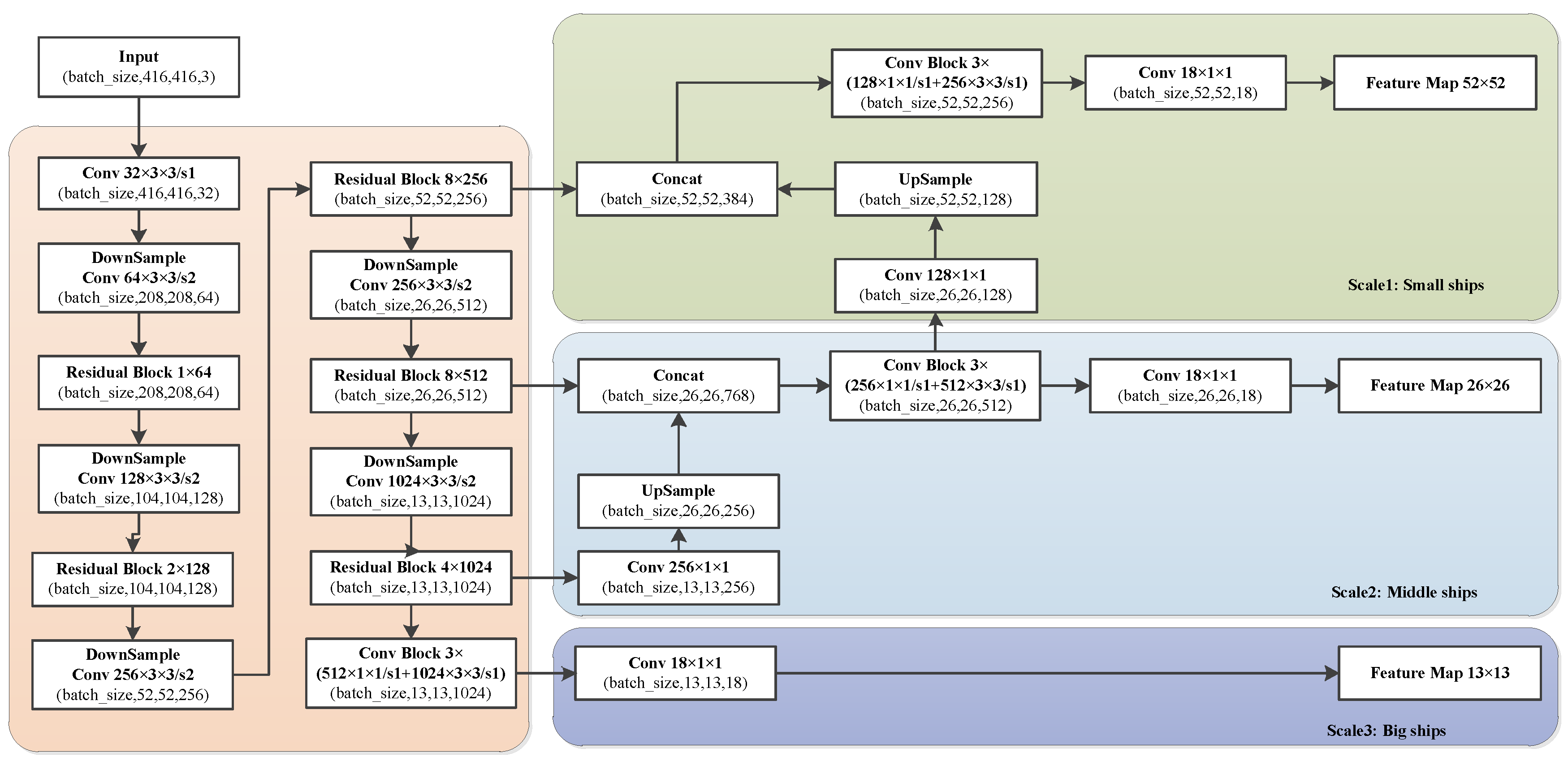
2.3.1. Feature Extraction Network.

The basic unit of the feature extraction network is DBL, which is composed of three different layers of darknet convolution, batch normalization (BN) and Leaky ReLU. DBL stands for darknet convolution + BN + Leaky Relu.
The feature extraction network uses residual connection in the backbone inspired by the residual network. The residual structure alleviates the problem of gradient disappearance in model training [33]. Therefore, the convolutional neural network can be stacked very deep. Due to the usage of residual connections, our model is easier to converge. By introducing a shortcut branch to the residual block, the network fit the residual mapping instead of directly fit the mapping. Compared with direct optimization mapping, it is easier to optimize residual mapping. The batch normalization layer is used to change the data distribution to avoid the parameters falling into the saturation zone. The batch normalization layer makes the network easier to converge during the training process. Leaky rectified linear unit (Leaky ReLU) is the activation function of feature extraction network.

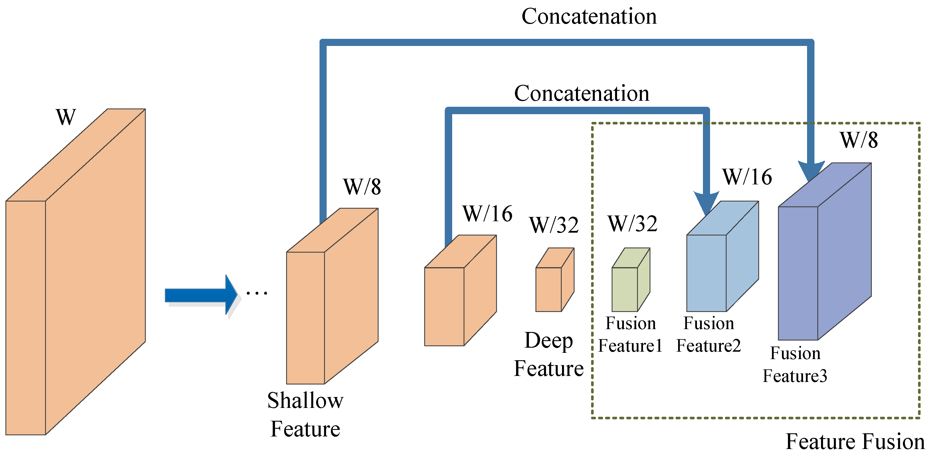
2.3.2. Convolutional Feature Fusion

Due to the different shooting distance of aerial remote sensing images, the size of the ship target is different. In the same reconnaissance field, there will also be ships of different scales. Therefore, our ship detection method is required to be scale invariant.
The convolutional feature fusion structure fuses shallow convolutional features and deep convolutional features, generating three kinds of fusion ship target feature: fusion feature 1, fusion feature 2 and fusion feature 3, inspired by the experience of feature pyramid networks (FPN) [34] and SSD. Figure 8 is the structure of convolutional feature fusion. As is shown in Figure 8, if the size of input image is W × W, the size of the fused convolution feature is W/8, W/16 and W/32. The deep convolution feature needs to be upsampled before fusion with shallow feature. The concatenation operation uses channel fusion instead of element-level fusion like FPN algorithm. The fusion of different levels of convolution features can better use the fine-grained features and semantic features of the ship, achieving multi-scale detection of ships.
CFF-SDN uses multi-scale convolution feature fusion, which is very effective for detection of small objects like remote sensing ships. CFF-SDN performs detection at three different scales. The feature maps in our proposed model combine fine-grained information from shallow layers and semantic information from deep layers. Fine-grained information contains more detailed features of ships, which is very conducive to the detection of small targets. This network structure allows the network to use fused features for detection, which helps us greatly improve the accuracy of small target detection.
The anchor design in this paper is inspired by YOLOv3, but it is very different from YOLOv3. Each grid cell in the YOLOv3 detection layers has three anchors of different sizes. There is only one type of detection target involved in this paper, and the ships in remote sensing images are mostly small and medium. CFF-SDN model has three kinds of fusion feature and performs prediction three times. The first prediction has a large receptive field, and two anchor boxes are allocated for prediction. The second prediction has a medium receptive field, and three anchor boxes are allocated for prediction. The third prediction has a small receptive field, and four anchor boxes are allocated for prediction. The anchor design of the CFF-SDN model is shown in Table 2. The dense anchor boxes can effectively improve the recall rate of the network, which are conducive to the detection of small ships. We use the k-means clustering algorithm to cluster the ship sizes of the DSDR dataset. Nine anchor boxes of preset sizes are generated for classification and bounding box regression, respectively (17 × 21), (22 × 51), (31 × 109), (48 × 29), (51 × 61), (68 × 118), (100 × 50), (144 × 102), (285 × 278).
There is only one type of detection target in our paper, that is, ships on the sea. In addition, their sizes are mostly small and medium, and the number of prior boxes allocated in the network depth information is increased to improve the detection accuracy and performance of small targets. The size of the ship targets in the images are mostly small and medium. By increasing the number of prior frame allocations in the network depth information, the detection accuracy and performance for small targets can be improved.

2.3.3. Soft NMS

Non-maximum suppression (NMS) plays a very important role in the field of target tracking and object detection. NMS is an algorithm designed to remove duplicate prediction boxes, which can effectively improve the detection performance of ship targets. We select the prediction box with the highest score in the neighborhood and suppress the prediction boxes which have lower scores with the assistance by NMS. The processing of NMS depends on the adjustment of the intersection over the union (IOU) threshold. The predicted box is drawn in green while the ground-truth box is drawn in red. IOU is the intersection over the union, the range of IOU is 0 to 1. Figure 9 shows the IOU between the prediction box and the ground-truth box.
However, violently eliminating the prediction boxes that do not have the highest score is the major problem of NMS. In the optical remote sensing images during ocean surveillance, especially in areas near ports, or when a fleet performs jointly missions, a ship will be surrounded by ships nearby, even obscured by other ship targets. Therefore, as is shown in Figure 10, the prediction boxes of nearby ships may exceed the preset overlap threshold. As a result, the ship’s prediction box will be suppressed, causing the loss of ship targets. This situation causes the missed detection rate to be very high, affecting the mean average precision.
To solve this problem, soft NMS is used to remove redundant prediction boxes. Unlike traditional NMS, soft does not directly zeroing the scores of high overlap detections, instead, it is assigned a lower score, so the ship target in this prediction box can still be detected. Soft NMS is denoted as follows:
s i = { s i I O U ( b h , b i ) < N t s i ( 1 I O U ( b h , b i ) ) I O U ( b h , b i ) N t
where si is detection scores; bh represents the prediction box with the highest score; bi represents other prediction boxes; IOU(bh, bi) is the intersection-over-union between the prediction box bh and bi; Nt represents IOU threshold. The implementation of soft NMS is shown in Figure 11.

2.3.4. Loss Function

The CFF-SDN is an end-to-end model, and the result of model is to provide the localization, category, and confidence of the prediction box. The total loss is divided into three parts, which are localization loss, classification loss, confidence loss, which is expressed as:
Loss = λ loc L loc + λ clc L cls + λ conf L conf
where λ loc ,   λ clc ,   λ conf are the weights of different kinds of losses. CFF-SDN only has one anchor box responsible for predicting an object within a ground-truth box. The loss regarding localization of prediction box contains the loss of location of the center point, the loss of width and height of the anchor box, which is defined as:
L loc = i = 0 S 2 j = 0 B l ij ship [ ( x i   x ^ i ) 2 + ( y i   y ^ i ) 2 ] + i = 0 S 2 j = 0 B l ij ship [ ( w i   w ^ i ) 2 + ( h i   h ^ i ) 2 ]
where l ij ship denotes whether the anchor box j of grid cell i contains a ship. If the anchor box contains a ship, l ij ship set to 1, otherwise set to 0.
When the anchor box is responsible for a ground-truth object, it causes losses for classification. The classification losses are defined as:
L cls = i = 0 S 2 l ij ship c classes [ p i ( c )   p ^ i ( c ) ] 2
The confidence loss consists of two parts, including the confidence loss when the anchor includes a ship and the confidence loss when the anchor does not include a ship. The weight of the confidence loss when the anchor does not include ship needs to be appropriately reduced, so λ noship < 1 . The confidence loss is expressed as:
L conf = i = 0 S 2 j = 0 B l ij ship ( C i   C ^ i ) 2 + λ noship i = 0 S 2 j = 0 B l ij noship ( C i   C ^ i ) 2

2.4. Model Pruning

Although large network structures have a strong representation power, they consume a lot of resources and affect the detection speed. In this paper, a method is proposed to prune the model. The channels with small scaling factors are pruned in the trained network. The channel-wise sparsity is applied to the optimization objective, so the channel pruning process is very smooth. The removal of redundant channels does not affect the accuracy. Therefore, after pruning, we can obtain a compact model with considerable accuracy.
Figure 12 shows the method to compress the CFF-SDN model by pruning. A scaling factor for each channel is introduced to the network. The scaling factor is multiplied to the output of channel. Then, we train the network weights and these scaling factors together and perform sparse regularization on them. Finally, we prune the channels with small scaling factors. The training objective of our method is defined by:
L = ( x , y ) l ( f ( x , W ) , y ) + λ γ Γ g ( γ )
where ( x , y ) represents training input and target output, W represents the model weights, the first term is consistent with the normal training loss of the model, g ( ) is a sparsity-induced penalty on the scaling factors, λ is responsible for the balance between the two terms. When a channel needs pruning, we remove all input and output connections for this channel, so that we can obtain a slim network. The pruned network can significantly reduce the inference time at runtime.

3. Experiments and Results

3.1. Model Training

We trained the CFF-DSN model on DSDR dataset. The DSDR dataset contains optical remote sensing images and ships in the images have different sizes and orientations. Due to the diversity of the dataset, the model is highly generalized on the test set and it is very robust to other scenarios. We trained our deep learning model CFF-SDN on the training set and validation set. The training parameters for CFF-DSN model are listed in Table 3.
Some ship detection results on DSDR dataset are displayed in Figure 13. To be fair, the experiments are conducted on the same platform. The models were trained and tested using a PC with Intel Xeon E5-2678 v3 @ 2.5GHz × 12 and 32 GB of RAM memory, and the GPU was NVIDIA RTX 2080Ti with 11G memory and using CUDA10.0. The operating system on the computer was 64-bit Ubuntu 18.04. Our experiments are performed on the PyCharm [35] software development platform, with Python 3.6 language. The result of Figure 13 is the performance of our model on the test set.
Most of the ships on the sea are small targets, and the CFF-SDN ship detection model is especially designed for the detection of small targets. CFF-SDN uses multi-scale convolution feature fusion, which is very effective for detection of small objects like remote sensing ships. Our model uses the k-means clustering algorithm to cluster the ship sizes of the DSDR dataset, and the number of priori boxes allocated in the network depth information is increased to improve the detection accuracy and performance of small targets. Our model achieved good results for the detection of small targets in remote sensing images. The small target detection results of CFF-SDN model on DSDR dataset are displayed in Figure 14. It can be seen from Figure 14 that even for small targets with pixels smaller than 7 × 7, our model can detect and recognize ships very well. It can be found from Figure 14 that our model can reliably detect small ships in different directions and attitudes.

3.2. Model Evaluation

To evaluate the overall performance of our model after detection, we use the precision, recall, F1 score and the mean of average precision (mAP) to analyze the performance of our proposed ship detection model quantitatively.
The precision is the ratio of true positives in all prediction boxes. The recall is the ratio of the ships that are detected correctly to the number of all ground-truth samples. As for ship detection, high accuracy and recall are both very important. However, the precision and recall indicators sometimes contradict each other, so we need to consider them comprehensively. F1 score is a comprehensive reflection of precision and recall. It is the weighted average of precision and recall. The precision, recall and F1 score are defined as follows:
precision = TP TP + FP
recall = TP TP + FN
F 1 = 2 × precision × recall precision + recall
where TP represents the number of true positives, which is when the detected ship is actually a ship target. FP represents the number of false positives, which is when a ship is detected, but the real value is not a ship. FN represents the number of false negatives, indicating a ship is not detected, but the result is a ship [36]. Precision is the ratio of detected true ships to all detected targets by the model. Recall is the ratio of the detected true ships to the total number (ground truth) of ships.
When the recall is high, the precision is very low. When the precision is high, the recall is often low. mAP comprehensively considers the precision and different recalls; it does not have any preference for precision or recall. mAP represents the area under the precision-recall curve and reflects the global performance of models, which is defined as:
mAP = 0 1 PdR

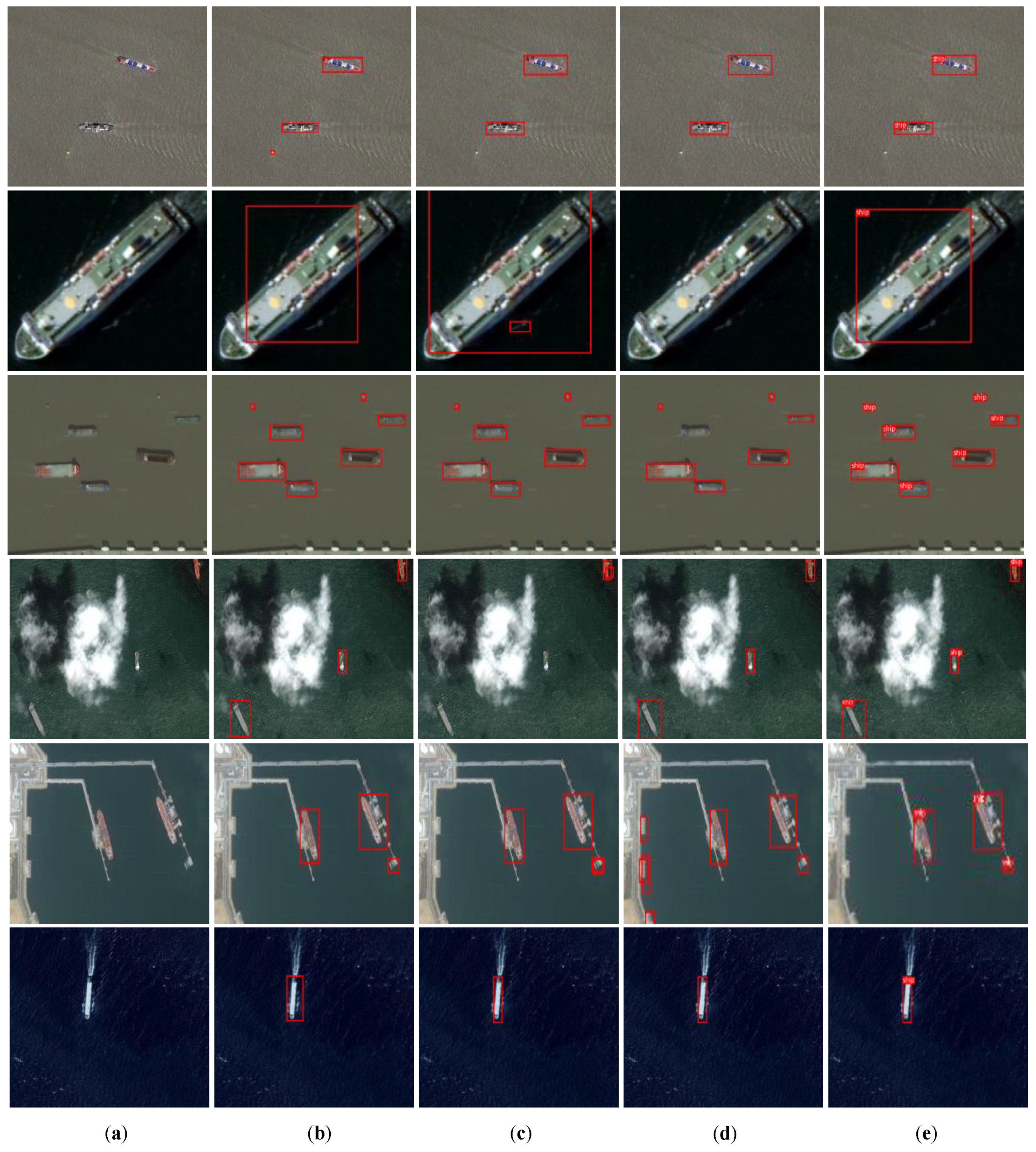
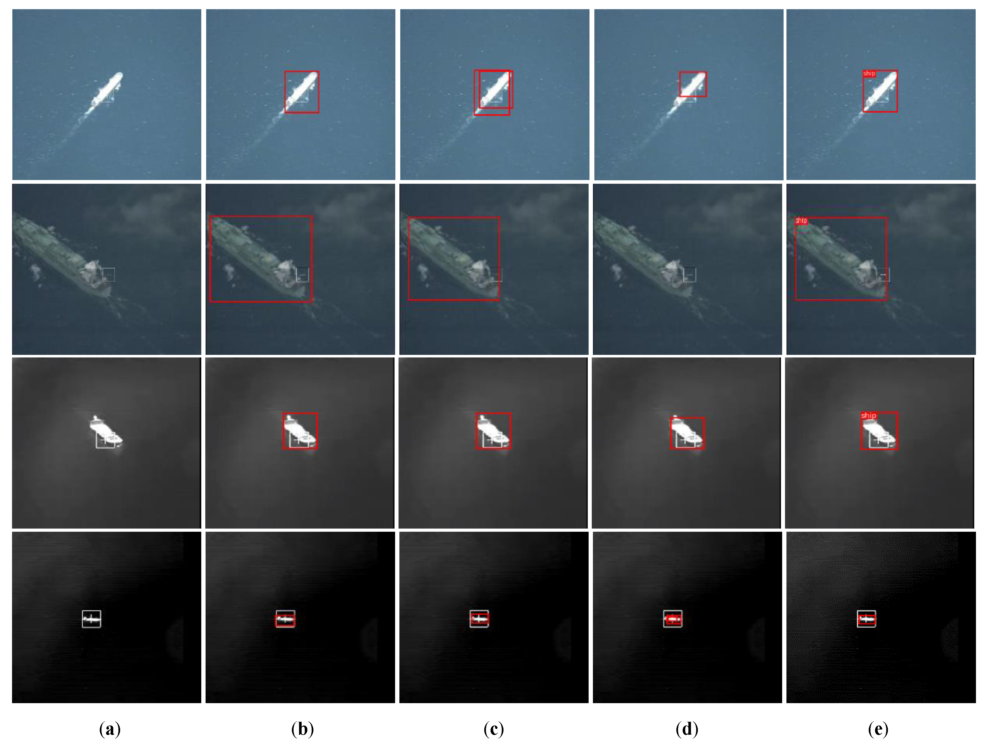
3.3. Comparison with Other Methods

CFF-SDN adopts convolutional feature fusion network, which can combine multi-layer ship features. The feature maps in our proposed model combine fine-grained information from shallow layers and semantic information from deep layers. Therefore, the CFF-SDN model is more suitable for the detection of multi-scale ships. At the same time, CFF-SDN can solve the problem of adjacent ship detection through soft NMS. To verify the superiority of the method we proposed, we compare the performance of our model with other state-of-the-art natural image object detection frameworks, such as Faster Regions Convolution Neural Network (Faster R-CNN), Single Shoot MultiBox Detector (SSD), You Only Look Once v3: An Incremental Improvement (YOLOv3). The size of input images is uniformly scaled to 416 × 416.
Figure 15 shows the detection results of satellite remote sensing images from different models, including Faster R-CNN, SSD, YOLOv3, and our proposed method, CFF-SDN. In Figure 15, the first row is affected by flare near the ship, leading to the Faster R-CNN generates a false alarm. The scale of the ship target in the second row in Figure 15 is relatively large, almost filling the entire image. In this case, it is difficult to detect or locate ship. The SSD mistakes the wave for ship, resulting in a false alarm. While the YOLOv3 failed to detect the ship, causing a missed detection. Our proposed model CFF-SDN and Faster R-CNN can detect the ship, but the localization of ship is not so accurate. In the third row, the scale of the ship varies greatly, and some ships are similar to the background. YOLOv3 did not detect the ship that similar to the background. As can be seen from the fourth row, SSD is seriously interfered with by the cloud. In the fifth row, the docking facility interferes with the detection of ship, causing the YOLOv3 algorithm to misunderstand the port facility as a ship and generates a false alarm. For example, in the sixth row, the detection and localization effects of each model are very good under simple backgrounds. Compared with other models, it is found that our proposed model CFF-SDN achieves better performance, because it adopts a convolutional feature fusion network, and uses multiple feature maps of different scales for detection and regression, simultaneously uses multiple strategies for data enhancement. All these measures mean that the model is able to detect ships with multiple scales, and can suppress the interference caused by clouds, landing facilities, ripples, and flares. The experimental results show that our model is very robust to various environments and interference.
Figure 16 shows the detection results of aerial remote sensing images from different models. The first row and second row are the detection results of visible light remote sensing images; it can be seen that the SNR of these images is quite low, and this situation is very common due to the influence of water vapor near sea. In the first row, disturbed by wake while the ship is sailing, SSD generates redundant detection, and YOLOv3 does not give the precise location of the ship. The last two rows are detection results of aerial infrared remote sensing images. Because the background is relatively simple, each model obtains a good classification and localization effect. Experiments show that the CFF-SDN model can detect remote sensing images of different spectrums very well. By using affine transformation to enrich ships with different perspectives in the dataset, the model has a good detection effect on ships with different perspectives in aerial remote sensing images.
For each detection framework participating in the comparison, we train DSDR dataset respectively and calculate the mAP value of the detection results. The mean average precisions of different models are shown in Table 4.
As shown in Table 4, Faster R-CNN is a two-stage detection framework, it has a Region Proposal Network (RPN) before class prediction and object localization, so it has higher mAP value than SSD and YOLOv3. Rotation Dense Feature Pyramid Networks (R-DFPN) [37] is also a two-stage object detector, similar to Faster R-CNN. R-DFPN adopt rotation anchors to avoid the side effects of NMS and overcome the difficulty of detecting densely arranged targets. However, complex scenes (such as a port or naval base) often contain objects with similar aspect ratios. such as roofs, container piles, and dock. Disturbances like roofs and docks will cause false alarms on the R-DFPN. Therefore, the F1 score of R-DFPN is only 89.6%, which is lower than our one-stage object detector CFF-SDN. The squeeze and excitation rank faster R-CNN (SER Faster R-CNN) [38] is designed to improve the ship detection performance in SAR images based on the Faster R-CNN by using a squeeze and excitation strategy. The SER Faster R-CNN extracted multiscale information based on VGG network. The F1 score of SER Faster R-CNN is 83.6%, and the F1 score of the CFF-SDN model is 7.7% higher than this. Because it is a two-stage object detector, the speed of it is relatively slow, and the inference time is 250 ms. Although the SSD outputs several different layers of feature maps for multi-scale detection, the information of single-layer feature maps is limited, so the accuracy rate is not very high. The improvement of SSD models, such as FA-SSD, introduces feature fusion and attention models to improve the performance of small target detection [20], but because there is only one detection layer, the accuracy rate is still not very high for ship detection in remote sensing images. ScratchDet [39] is another improvement method of SSD. The method integrated batch normalization to help the detector converge well. It can train SSD from scratch without pre-training weights. ScratchDet proposed the Root-ResNet backbone network, which achieved higher accuracy than SSD. However, the training time is 2.8 times that of SSD. The inference time is 37 ms, which is much higher than our CFF-SDN model. CFF-SDN uses data augmentation strategies to enrich the scale, perspective, and color information of ships, and uses convolutional feature fusion information of different layers for detection, making the CFF-SDN model have the highest mAP among these algorithms.
By changing the confidence threshold from 0 to 1, we can get different evaluation results. Figure 17 shows the precision–recall curves of different models for optical remote sensing image ship detection. The precision–recall curve goes up and to the right means the model has better ship detection performance. The precision–recall curve of CFF-SDN model is clearly above other curves. Therefore, the ship detection model CFF-SDN that we propose in this paper has better performance than Faster R-CNN, SSD and YOLOv3.
Table 5 shows the time cost of ship detection by different models. Due to Faster R-CNN being a two-stage method, it spends a lot of time generating regions of interest (ROIs), so the detection speed of Faster R-CNN is the slowest of these methods. The SR network with faster R-CNN yielded the very good results for small objects on satellite imagery; however, the detection speed of the network is slow [23], so it is difficult to deploy in engineering applications. SSD is a one-stage multibox detector, it takes 61 ms. YOLOv3 is a one-stage model, and it takes 22 ms. Since the CFF-SDN model uses a pruning strategy, it takes 9.4 ms, which is the least time-consuming of these methods. The removal of redundant channels does not affect the accuracy. Due to the slimming of the network, the inference time of the model can be reduced. Therefore, the proposed model pruning method can speed up the detection speed without reducing the accuracy. Before model pruning, the mAP of the ship detection model is 91.508%, and the average inference time is 20 ms. After model pruning, the mAP of CFF-SDN model is higher, which is 91.51%. It is found that mAP fluctuates up and down by 0.002% is a normal phenomenon in the experiment, so it can be considered that the mAP after model pruning is almost the same as normal training. As the model pruning makes the network slim, the average inference time is improved by 10.6 ms.

3.4. Effect of Data Preprocessing

The data preprocessing in our model includes data augmentation and atmospheric correction. Data augmentation methods for remote sensing images have been proposed to prevent the model from overfitting and increase the detection accuracy. Means like horizontal flipping, vertical flipping, random rotation, random scaling, random cropping or expansion are used to enrich the training samples. Color jittering is applied to adjust the contrast, brightness, saturation and hue of ship images. An affine transformation method is also proposed, which enables satellite images to be expanded to images with different viewing angles.
An atmospheric correction method based on the dark channel prior can well reduce the influence of atmospheric absorption and scattering on remote sensing images. After atmospheric correction, the ships in the remote sensing image are clearer, and the color fidelity of the ships is higher. The correction of atmospheric absorption and scattering helps improve the accuracy of ship detection.
We evaluated the impact of data preprocessing in the performance of CFF-SDN model. The size of input images is uniformly scaled to 416 × 416. Table 6 shows the effect of data augmentation and atmospheric correction for CFF-SDN model. The mAP of the CFF-SDN with data augmentation was 90.42%, while the mAP of CFF-SDN model without data augmentation was 88.84%. Through data augmentation, the mAP value is improved by 1.58%. The mAP of the CFF-SDN with atmospheric correction and data augmentation was 91.51%; through atmospheric correction, the mAP value was improved by 1.09%.
Figure 18 shows the precision–recall curves of CFF-SDN model with data preprocessing and CFF-SDN model without data preprocessing. The precision–recall curve of the CFF-SDN model with augmentation is much higher than the CFF-SDN model without augmentation. The precision–recall rate curve with image augmentation and atmospheric correction is the highest, which is closest to the upper right. This means that data augmentation and atmospheric correction are helpful for improving the accuracy of ship detection.

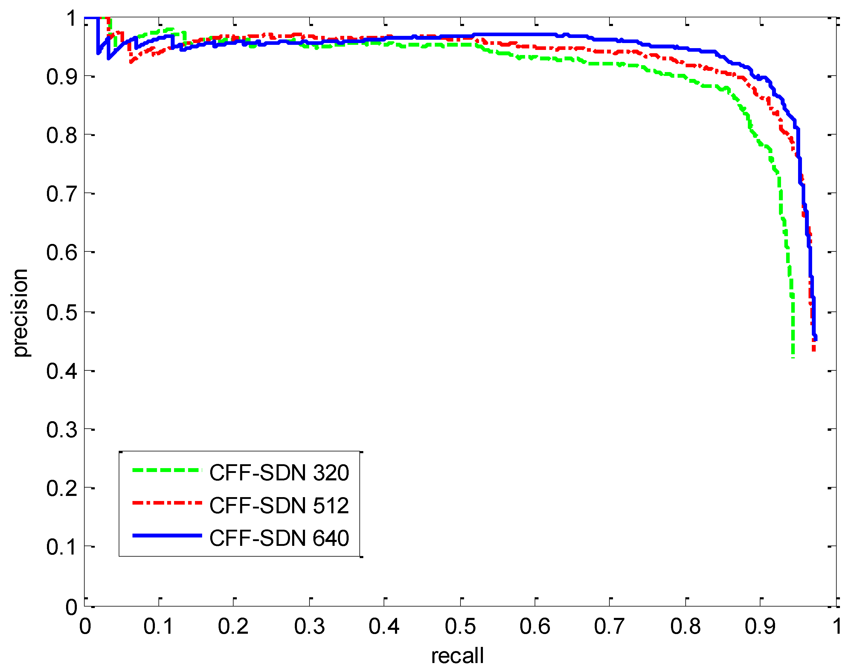
3.5. Performance Comparison of Different Image Sizes

We evaluated the impact of different image sizes in the performance of CFF-SDN model. To get images of different sizes, we resized the remote sensing images in the DSDR dataset to 320 × 320, 512 × 512, 640 × 640, respectively. The mAP of the CFF-SDN ship detection model was 88.61, 92.44 and 93.25 percent.
Table 7 shows the performance of CFF-SDN with different image sizes. In general, as the image size increases, the detection performance of the CFF-SDN model improves to a certain extent. However, the computational complexity of the model increadses as the image size becomes larger. Billion floating point operations per second (BFLOPS) increased from 5.7 to 22.7, as the image width and height increased from 320 to 640. When we need to detect larger images, the CFF-SDN model requires greater inference time than detecting small images.
Figure 19 shows the precision–recall curves of CFF-SDN model for different image sizes. The precision–recall curve of 640 is much higher than others. This means that the larger the size of the images, the higher the accuracy of ship detection. In engineering application, we can select the appropriate input image size according to the required detection accuracy and allowable detection speed.

4. Discussion

Through comprehensive analysis and comparison with other models, our proposed CFF-SDN model was shown to be effective for ship detection in optical remote sensing images. The multi-layer convolutional feature fusion method is innovatively proposed, enhancing the fine-grained information and semantic information. It can be seen through experiments that our model has excellent performance in terms of detection accuracy and speed.
We proposed the CFF-SDN model, which can fuse fine-grained information from shallow layers and semantic information from deep layers. This network architecture is very beneficial for the detection of small objects like ships in remote sensing images. Due to the use of fused feature maps for regression and classification, the CFF-SDN model has good adaptability to the multi-scale changes of ships. Table 3 shows that the CFF-SDN model can achieve better performance than other object detectors.
Various data augmentation strategies are important measures for improving detection accuracy. Innovatively, affine transformation was used to change the perspective of satellite remote sensing images. As shown in Figure 5, the satellite image after affine transformation is very similar to the aerial remote sensing images taken from different perspectives. The use of rich satellite remote sensing images to improve the detection accuracy of aerial remote sensing images plays an important role in improving the overall detection accuracy.
As ships are often densely arranged on the sea, as shown in Figure 10, unlike traditional non-maximum suppression, we use soft NMS to suppress redundant prediction boxes, which increases the probability that the ship will be detected when closely arranged, effectively improves the recall rate of the model, and reduces missed detections.
Since our model adopts a model pruning strategy, the CFF-SDN model has a lower computational complexity. As shown in Table 4, our proposed model has a faster detection speed than the other compared models, and is thus more conducive to migration to the embedded platform, in order to achieve real-time ship target detection in engineering applications.
By comparing the many groups of experiments, it is verified that the CFF-SDN ship detection model can achieve high performance on detection accuracy, as shown in the precision–recall curves in Figure 17. However, ships sometimes sail in complex scenes, and the shapes and textures of interfering objects (such as islands, clouds) can change considerably. Sometimes the shape, color, and texture of clouds or islands are very similar to those of ships. These disturbances can cause false alarms in the detector, as shown in Figure 20.
Although CFF-SDN fully reuses feature information by fusing features from different layers, it is still not enough to eliminate all false alarms.
Both the training set and the test set contain harbor images, and the ship detection in these images is interfered with by the land. The ship detection results of harbor images containing land are shown in Figure 21. The CFF-SDN model can detect ships in the harbor. Although the model does not appear to be overfitting, the detection effect in the harbor images is not as good as that in the ocean images. The ships near the shore in Figure 21a–c are well detected. Three ships were detected in Figure 21d, but one ship docked on the shore was not detected. There are many interferences when detecting ships in the harbor, and the detection effect is lower than that of ships on the sea. The mAP would be significantly decreased when the trained model is applied to the harbor images. Enhancing the robustness of algorithms for ship detection in harbor is an important research topic in the future. We need to collect more harbor images to support the quantitative analysis of ship detection in the harbor.
The interferences of ship detection on different datasets are quite different. We collected several different datasets, including vehicle detection in aerial imagery (VEDAI) dataset [40], dataset for object detection in aerial images (DOTA) [41], and high-resolution remote sensing detection (HRRSD) dataset [42]. These datasets contain various types of targets such as airplanes, tractors, ships, trucks, etc. The ship images extracted from these datasets are detected by CFF-SDN model to detect ship images. In addition, the number of ships in these datasets is not as high as in our dataset DSDR. The ship detection results of CFF-SDN model on other datasets are shown in Figure 22.
It can be seen from Figure 22 that various types of ships in these datasets were detected, and no interfering objects such as harbor facilities were mistakenly detected as ships. The ship detection results on different datasets prove that our model is very robust. The detection result of the DOTA dataset in the first row of Figure 22 shows that the localization of the ship in the upper left corner is not accurate enough. In the future, the localization accuracy of the CFF-SDN model on other datasets needs to be improved.
Increasing the learning category is a better solution to this problem. Common disturbances such as clouds and islands are divided into separate categories. In addition to learn the target characteristics of the ships, the model also learns the characteristics of common interferers that cause false alarms to distinguish between ships and interference. The fusion of visible and infrared image information may be another idea for enhancing the recognition capability of the detector by comprehensively using the interference suppression effect of different spectrum bands to improve the performance of distinguishing ships from false alarms, but this depends on the linkage of the visible and infrared sensors, so as to obtain both visible and infrared images of the same scene.

5. Conclusions

In this paper, we proposed an end-to-end ship detection model that can effectively cope with various disturbances in optical remote sensing images, such as satellite remote sensing images, visible aerial remote sensing images, infrared aerial remote sensing images. Because our method uses a convolutional feature fusion network and multi-scale feature maps are used for regression and classification, it can detect ship with different sizes in remote sensing images. Our model uses the affine transformation method, so the CFF-SDN model can detect ships with different perspectives. A dark channel prior is adopted to solve the atmospheric correction on the sea scenes, removing the influence of the absorption and scattering of water vapor and particles in the atmosphere. Above all, in the feature extraction stage, the convolutional feature extraction network is used to obtain ship features from shallow to deep. Then, in the feature fusion stage, we integrate different levels of ship features through feature fusion network. Finally, soft NMS is applied to suppress redundant predictions. The model outputs the localization, classification and confidence of ships in the remote sensing images. Since the CFF-SDN model uses a pruning strategy, the detection speed is faster than other comparison models. Overall, the mAP of our proposed detection framework was 91.51% with resolution 416 × 416, and the average inference time was 9.4 ms. Our model has good performance for small target detection, and can detect ships with pixels as small as 7 × 7 in remote sensing images. The experimental results show that our model is robust, effective and fast, and can be used for real-time detection of ships.
In our future work, we plan to enrich the aerial remote sensing images in DSDR dataset to improve the training effect. On the other hand, transplant the model to the embedded platform to realize the engineering application of ship detection.

Author Contributions

Y.Z. and L.G. designed the proposed detection model. Y.Z. and F.X. collected the experimental data. Z.W. provided experimental equipment. Y.Z. drafted the manuscript. Y.Y. assisted in the experiment of atmospheric correction. F.X. and X.L. edited the manuscript. L.G. provided guidance to the project, reviewed the manuscript, and obtained funding to support this research. All authors have read and agreed to the published version of the manuscript.

Funding

This work was supported by the National Natural Science Foundation of China (Grant No. 61977059) and the Programs Foundation of Key Laboratory of Airborne Optical Imaging and Measurement, Chinese Academy of Science (Grant No. y3hc1sr141).

Acknowledgments

The authors would like to thank the editors and the reviewers for their valuable suggestions.

Conflicts of Interest

The authors declare no conflict of interest.

Abbreviations

CFF-SDNship detection network based on multi-layer convolutional feature fusion
DSDRdataset for ship detection in remote sensing images
SARsynthetic aperture radar
UAVsunmanned aerial vehicles
ROIsthe regions of interest
GBVSgraph-based visual Saliency
Faster R-CNNfaster regions convolution neural network
SSDsingle shot multi-box detector
YOLOyou only look once
NMSnon-maximum suppression
GSDground sampling distance
BNbatch normalization
Leaky ReLUleaky rectified linear unit
DBLdarknet convolution + BN + Leaky Relu
IOUintersection over the union
mAPthe mean of average precision
TPthe number of true positives
FPthe number of false positives
FNthe number of false negatives
BFLOPSbillion floating point operations per second
VEDAIvehicle detection in aerial imagery dataset
DOTAdataset for object detection in aerial images
HRRSDhigh-resolution remote sensing detection dataset

References

  1. He, H.; Lin, Y.; Chen, F.; Tai, H.-M.; Yin, Z. Inshore Ship Detection in Remote Sensing Images via Weighted Pose Voting. IEEE Trans. Geosci. Remote Sens. 2017, 55, 1–17. [Google Scholar] [CrossRef]
  2. Su, H.; Wei, S.; Liu, S.; Liang, J.; Wang, C.; Shi, J.; Zhang, X. HQ-ISNet: High-Quality Instance Segmentation for Remote Sensing Imagery. Remote Sens. 2020, 12, 989. [Google Scholar] [CrossRef] [Green Version]
  3. Dong, C.; Liu, J.; Xu, F. Ship Detection in Optical Remote Sensing Images Based on Saliency and a Rotation-Invariant Descriptor. Remote Sens. 2018, 10, 400. [Google Scholar] [CrossRef] [Green Version]
  4. Chang, Y.L.; Anagaw, A.; Chang, L.; Wang, Y.C.; Hsiao, C.Y.; Lee, W.H. Ship Detection Based on YOLOv2 for SAR Imagery. Remote Sens. 2019, 11, 786. [Google Scholar] [CrossRef] [Green Version]
  5. Itti, L.; Koch, C.; Niebur, E. A model of saliency-based visual attention for rapid scene analysis. IEEE Trans. Pattern Anal. Mach. Intell. 1998, 20, 1254–1259. [Google Scholar] [CrossRef] [Green Version]
  6. Harel, J.; Koch, C.; Perona, P. Graph-Based Visual Saliency. In Proceedings of the 20th Annual Conference on Neural Information Processing Systems, Vancouver, BC, Canada, 4–7 December 2006; pp. 545–552. [Google Scholar]
  7. Hou, X.; Zhang, L. Saliency Detection: A Spectral Residual Approach. In Proceedings of the 2007 IEEE Conference on Computer Vision and Pattern Recognition, Minneapolis, MN, USA, 17–22 June 2007. [Google Scholar]
  8. Achanta, R.; Hemami, S.S.; Estrada, F.J.; Susstrunk, S. Frequency-tuned salient region detection. In Proceedings of the 2009 IEEE Conference on Computer Vision and Pattern Recognition, Miami, FL, USA, 20–25 June 2009; pp. 1597–1604. [Google Scholar]
  9. Li, S.; Zhou, Z.; Wang, B.; Wu, F. A Novel Inshore Ship Detection via Ship Head Classification and Body Boundary Determination. IEEE Geosci. Remote Sens. Lett. 2016, 13, 1–5. [Google Scholar] [CrossRef]
  10. Xu, F.; Liu, J.; Sun, M.; Zeng, D.; Wang, X. A Hierarchical Maritime Target Detection Method for Optical Remote Sensing Imagery. Remote Sens. 2017, 9, 280. [Google Scholar] [CrossRef] [Green Version]
  11. Margarit, G.; Tabasco, A. Ship Classification in Single-Pol SAR Images Based on Fuzzy Logic. IEEE Trans. Geosci. Remote Sens. 2011, 49, 3129–3138. [Google Scholar] [CrossRef]
  12. Qi, S.; Ma, J.; Lin, J.; Li, Y.; Tian, J. Unsupervised Ship Detection Based on Saliency and S-HOG Descriptor from Optical Satellite Images. IEEE Geosci. Remote Sens. Lett. 2015, 12, 1451–1455. [Google Scholar] [CrossRef]
  13. Ren, S.; He, K.; Girshick, R.; Sun, J. Faster R-CNN: Towards Real-Time Object Detection with Region Proposal Networks. IEEE Trans. Pattern Anal. Mach. Intell. 2017, 39, 1137–1149. [Google Scholar] [CrossRef] [Green Version]
  14. Liu, W.; Anguelov, D.; Erhan, D.; Szegedy, C.; Reed, S.; Fu, C.; Berg, A.C. SSD: Single Shot MultiBox Detector. In Proceedings of the 14th European Conference on Computer Vision, Amsterdam, The Netherlands, 8–16 October 2016; pp. 21–37. [Google Scholar]
  15. Simonyan, K.; Zisserman, A. Very Deep Convolutional Networks for Large-Scale Image Recognition. In Proceedings of the 2014 IEEE Conference on Computer Vision and Pattern Recognition, Columbus, OH, USA, 23–28 June 2014. [Google Scholar]
  16. Redmon, J.; Divvala, S.K.; Girshick, R.; Farhadi, A. You Only Look Once: Unified, Real-Time Object Detection. In Proceedings of the 2016 IEEE Conference on Computer Vision and Pattern Recognition, Las Vegas, NV, USA, 27–30 June 2016; pp. 779–788. [Google Scholar]
  17. Redmon, J.; Farhadi, A. YOLO9000: Better, Faster, Stronger. In Proceedings of the 2017 IEEE Conference on Computer Vision and Pattern Recognition, Honolulu, HI, USA, 21–26 July 2017; pp. 6517–6525. [Google Scholar]
  18. Ju, M.; Luo, H.; Wang, Z.; Hui, B.; Chang, Z. The application of improved YOLO V3 in multi-scale target detection. Appl. Sci. 2019, 9, 3775. [Google Scholar] [CrossRef] [Green Version]
  19. Yi, Z.; Yongliang, S.; Jun, Z. An improved tiny-yolov3 pedestrian detection algorithm. Optik 2019, 183, 17–23. [Google Scholar] [CrossRef]
  20. Lim, J.; Astrid, M.; Yoon, H.; Lee, S. Small Object Detection using Context and Attention. In Proceedings of the 2019 IEEE Conference on Computer Vision and Pattern Recognition, Long Beach, CA, USA, 15–21 June 2019. [Google Scholar]
  21. Everingham, M.; Van Gool, L.; Williams, C.K.I.; Winn, J.; Zisserman, A. The Pascal Visual Object Classes (VOC) Challenge. Int. J. Comput. Vis. 2010, 88, 303–338. [Google Scholar] [CrossRef] [Green Version]
  22. Lin, T.Y.; Maire, M.; Belongie, S.; Hays, J.; Perona, P.; Ramanan, D.; Dollár, P.; Zitnick, C.L. Microsoft COCO: Common Objects in Context. In Proceedings of the 13th European Conference, Zurich, Switzerland, 6–12 September 2014; pp. 740–755. [Google Scholar]
  23. Rabbi, J.; Ray, N.; Schubert, M.; Chowdhury, S.; Chao, D. Small-Object Detection in Remote Sensing Images with End-to-End Edge-Enhanced GAN and Object Detector Network. Remote Sens. 2020, 12, 1432. [Google Scholar] [CrossRef]
  24. Shao, Z.; Wang, L.; Wang, Z.; Du, W.; Wu, W. Saliency-Aware Convolution Neural Network for Ship Detection in Surveillance Video. IEEE Trans. Circuits Syst. Video Technol. 2020, 30, 781–794. [Google Scholar] [CrossRef]
  25. Nie, X.; Duan, M.; Ding, H.; Hu, B.; Wong, E.K. Attention Mask R-CNN for Ship Detection and Segmentation from Remote Sensing Images. IEEE Access 2020, 8, 9325–9334. [Google Scholar] [CrossRef]
  26. Li, Y.; Peng, C.; Chen, Y.; Jiao, L.; Zhou, L.; Shang, R. A Deep Learning Method for Change Detection in Synthetic Aperture Radar Images. IEEE Trans. Geosci. Remote Sens. 2019, 57, 1–13. [Google Scholar] [CrossRef]
  27. An, Q.; Pan, Z.; You, H. Ship Detection in Gaofen-3 SAR Images Based on Sea Clutter Distribution Analysis and Deep Convolutional Neural Network. Sensors 2018, 18, 334. [Google Scholar] [CrossRef] [Green Version]
  28. Zhang, X.; Yu, Q.; Yu, H. Physics Inspired Methods for Crowd Video Surveillance and Analysis: A Survey. IEEE Access 2018, 6, 66816–66830. [Google Scholar] [CrossRef]
  29. Zhang, X.; Shu, X.; He, Z. Crowd panic state detection using entropy of the distribution of enthalpy. Phys. A Stat. Mech. Its Appl. 2019, 525, 935–945. [Google Scholar] [CrossRef]
  30. Song, P.; Qi, L.; Qian, X.; Lu, X. Detection of ships in inland river using high-resolution optical satellite imagery based on mixture of deformable part models. J. Parallel Distrib. Comput. 2019, 132, 1–7. [Google Scholar] [CrossRef]
  31. Wang, Z.; Yang, T.; Zhang, H. Land contained sea area ship detection using spaceborne image. Pattern Recognit. Lett. 2020, 130, 125–131. [Google Scholar] [CrossRef]
  32. He, K.; Sun, J.; Tang, X. Single image haze removal using dark channel prior. In Proceedings of the 2009 IEEE Conference on Computer Vision and Pattern Recognition, Miami, FL, USA, 20–25 June 2009; pp. 1956–1963. [Google Scholar]
  33. He, K.; Zhang, X.; Ren, S.; Sun, J. Deep Residual Learning for Image Recognition. In Proceedings of the 2016 IEEE Conference on Computer Vision and Pattern Recognition, Las Vegas, NV, USA, 27–30 June 2016; pp. 770–778. [Google Scholar]
  34. Lin, T.; Dollar, P.; Girshick, R.; He, K.; Hariharan, B.; Belongie, S. Feature Pyramid Networks for Object Detection. In Proceedings of the 2017 IEEE Conference on Computer Vision and Pattern Recognition, Honolulu, HI, USA, 21–26 July 2017; pp. 936–944. [Google Scholar]
  35. Pycharm. Available online: http://www.jetbrains.com/pycharm/ (accessed on 1 January 2020).
  36. Zhang, X.; Ma, D.; Yu, H.; Huang, Y.; Howell, P.; Stevens, B. Scene perception guided crowd anomaly detection. Neurocomputing 2020, 414, 291–302. [Google Scholar] [CrossRef]
  37. Yang, X.; Sun, H.; Fu, K.; Yang, J.; Sun, X.; Yan, M.; Guo, Z. Automatic ship detection in remote sensing images from google earth of complex scenes based on multiscale rotation dense feature pyramid networks. Remote Sens. 2018, 10, 132. [Google Scholar] [CrossRef] [Green Version]
  38. Lin, Z.; Ji, K.; Leng, X.; Kuang, G. Squeeze and excitation rank faster R-CNN for ship detection in SAR images. IEEE Geosci. Remote Sens. Lett. 2018, 16, 751–755. [Google Scholar] [CrossRef]
  39. Zhu, R.; Zhang, S.; Wang, X.; Wen, L.; Shi, H.; Bo, L.; Mei, T. ScratchDet: Training single-shot object detectors from scratch. In Proceedings of the 2019 IEEE Conference on Computer Vision and Pattern Recognition, Long Beach, CA, USA, 15–21 June 2019; pp. 2268–2277. [Google Scholar]
  40. Razakarivony, S.; Jurie, F. Vehicle detection in aerial imagery: A small target detection benchmark. J. Vis. Commun. Image Represent. 2016, 34, 187–203. [Google Scholar] [CrossRef]
  41. Xia, G.S.; Bai, X.; Ding, J.; Zhu, Z.; Belongie, S.; Luo, J.; Datcu, M.; Pelillo, M.; Zhang, L. DOTA: A large-scale dataset for object detection in aerial images. In Proceedings of the 2018 IEEE Conference on Computer Vision and Pattern Recognition, Salt Lake City, UT, USA, 18–22 June 2018; pp. 3974–3983. [Google Scholar]
  42. Zhang, Y.; Yuan, Y.; Feng, Y.; Lu, X. Hierarchical and robust convolutional neural network for very high-resolution remote sensing object detection. IEEE Trans. Geosci. Remote Sens. 2019, 57, 5535–5548. [Google Scholar] [CrossRef]
Figure 1. Flow chart of the proposed ship detection network-based convolutional feature fusion (CFF-SDN). The object detection framework consists of a feature extraction network, a feature fusion network, classification and regression. The detection result contains the classification and localization of ships.
Remotesensing 12 03316 g001
Figure 2. Some optical remote sensing images in DSDR dataset. The background of the ships is particularly complex, the ships are surrounded or blocked by clouds (a,b), there is island near the ship (c), interference caused by ripple (df), the effect of uneven lighting (e), ship docked at the port (f), ships from different perspectives (gi).
Remotesensing 12 03316 g002
Figure 3. The labeling example of the ships’ ground-truth boxes uses the annotation tool LabelImg. (a) The labeling example of the ship’s ground-truth boxes in ocean image; (b) The labeling example of the ship’s ground-truth boxes in harbor scene.
Remotesensing 12 03316 g003
Figure 4. The image augmentation of the training set. (a) Original image; (b) Horizontal flipping; (c) Contrast adjustment; (d) Brightness adjustment; (e) Saturation adjustment; (f) Hue adjustment; (g) Random rotation; (h) Random cropping; (i) Random scaling.
Remotesensing 12 03316 g004
Figure 5. Images from different perspectives produced by the affine transformation of satellite remote sensing images. (a) Original image. (bf) Different perspective images generated by affine transformation.
Remotesensing 12 03316 g005
Figure 6. Atmospheric correction effect of satellite remote sensing images and aerial remote sensing images. (ad) Original image. (eh) Ship images after atmospheric correction. (a,d) Aerial remote sensing images. (e,h) Atmospheric correction effects of aerial remote sensing images. (b,c) Satellite remote sensing images. (e,h) Atmospheric correction effects of satellite remote sensing images.
Remotesensing 12 03316 g006
Figure 7. The architecture of the convolutional feature fusion ship detection network (CFF-SDN). The residual block and the convolution block are used to extract feature of ship targets. In the convolutional feature fusion network, scale 1 detects small ships, scale 2 detects medium ships, and scale 3 detects large ships.
Remotesensing 12 03316 g007
Figure 8. Convolutional feature fusion structure. Concatenation operations are used to fuse shallow convolutional features and deep convolutional features, which is beneficial to achieve multi-scale detection of ships. Meanwhile, fused features are helpful for detecting small targets.
Remotesensing 12 03316 g008
Figure 9. Intersection over the union (IOU) between the prediction box and the ground-truth box.
Remotesensing 12 03316 g009
Figure 10. NMS reduces the recall rate of ship detection and causes missed detection.
Remotesensing 12 03316 g010
Figure 11. The implementation of the soft NMS algorithm.
Remotesensing 12 03316 g011
Figure 12. The model is compressed by pruning. During training, the model automatically recognizes unimportant channels. The channels with small scaling factor will be pruned. After pruning, the model will be more compact, occupy less memory and run faster, without loss of accuracy.
Remotesensing 12 03316 g012
Figure 13. Ship detection results of CFF-SDN model on DSDR dataset. (ad) Ship detection results of visible light images. (e,f) Ship detection results of infrared images. (gi) Detection results of ships of different shapes on visible light images.
Remotesensing 12 03316 g013
Figure 14. Small target detection results of CFF-SDN model on DSDR dataset. (a) The pixels of the ship target in the image are less than 7 × 7; (b) The sizes of the two targets are 22 × 18 and 24 × 76 respectively; (c) The pixels of the ship target are smaller than 36 × 51; (d) The ship targets in the image are very small, the smallest is only 6 × 10. (eh) are the detection results of small target ships in the images (ad), and all small ships in (eh) have been detected by our model. The CFF-SDN model can detect all small targets in the image.
Remotesensing 12 03316 g014
Figure 15. Detection results of satellite remote sensing images from different models. (a) Original Images; (b) Faster Regions Convolution Neural Network (Faster R-CNN); (c) Single Shoot MultiBox Detector (SSD); (d) You Only Look Once v3: An Incremental Improvement (YOLOv3); (e) Convolutional Feature Fusion Ship Detection Network (CFF-SDN).
Remotesensing 12 03316 g015
Figure 16. Detection results of aerial remote sensing images from different models. (a) Original Images; (b) Faster R-CNN; (c) SSD; (d) YOLOv3; (e) CFF-SDN. The first row and the second row are detection results of visible light images, the last two rows are detection results of infrared images.
Remotesensing 12 03316 g016
Figure 17. Precision–recall curves of Faster R-CNN, SSD, YOLOv3 and CFF-SDN.
Remotesensing 12 03316 g017
Figure 18. Precision–recall curves of CFF-SDN model with data preprocessing and CFF-SDN model without data preprocessing.
Remotesensing 12 03316 g018
Figure 19. Precision–recall curves of CFF-SDN model for different image sizes.
Remotesensing 12 03316 g019
Figure 20. Examples of false alarms caused by different disturbances. (a) Islands; (b) Clouds.
Remotesensing 12 03316 g020
Figure 21. Examples of ship detection results of harbor images containing land. The ships near the shore in the images (ac) are well detected. Three ships were detected in (d), but one ship docked on the shore was not detected. There are many interferences when detecting ships in the harbor, and the detection effect is lower than that of ships on the sea.
Remotesensing 12 03316 g021
Figure 22. Ship detection results of CFF-SDN model on other datasets. (a) Ship detection results for vehicle detection in aerial imagery (VEDAI) dataset; (b) Ship detection results for dataset for object detection in aerial images (DOTA); (c) Ship detection results for high-resolution remote sensing detection (HRRSD) dataset; (d) Ship detection results for our DSDR dataset.
Remotesensing 12 03316 g022
Table 1. The division of data set for ship detection in remote-sensing images (DSDR).
DatasetNumber of SamplesNumber of Ships
Training set11462910
Validation set369959
Test set369950
Total18844819
Table 2. The anchor design of the CFF-SDN model.
Prediction OrderReceptive FieldNumber of Anchor Boxes
1Large2
2Medium3
3Small4
Table 3. Hyper-parameters for training CFF-SDN model. The optimizer used in model was Adam.
Hyper-ParameterValue
Learning rate0.001
Learning change steps400,000, 450,000
Learning change scales0.1, 0.1
Batch size16
Momentum0.9
Decay0.0005
Epochs2000
Table 4. The precision, recall, F1 score and the mean of average precision (mAP) of different models for ship detection in optical remote sensing images.
ModelPrecisionRecallF1 ScoremAP
Faster R-CNN83.3289.6586.3787.81
SSD77.3583.3680.2481.53
YOLOv378.0984.6281.2282.73
CFF-SDN87.2393.1190.0791.51
Table 5. Average time cost of ship detection by different models.
ModelFaster R-CNNSSDYOLOv3CFF-SDN
(Before Pruning)
CFF-SDN
(After Pruning)
Time (ms)1406122209.4
Table 6. The effect of data augmentation and atmospheric correction for CFF-SDN model.
ModelData AugmentationAtmospheric CorrectionPrecisionRecallF1 ScoremAP
CFF-SDN××85.0291.1287.9688.84
×86.1692.2589.1090.42
87.2393.1190.0791.51
Table 7. Performance of CFF-DSN with different image size.
ModelImage SizePrecisionRecallF1 ScoremAPInference TimeBFLOPS
CFF-DSN320 × 32082.9491.7387.1188.618.75.8
512 × 51288.9293.6891.2392.4411.814.7
640 × 64089.9894.6292.2493.2514.622.9

