Abstract
In recent decades, land use/cover change (LUCC) due to urbanization, deforestation, and desertification has dramatically increased, which changes the global landscape and increases the pressure on the environment. LUCC not only accelerates global warming but also causes widespread and irreversible loss of biodiversity. Therefore, LUCC reconstruction has important scientific and practical value for studying environmental and ecological changes. The commonly used LUCC reconstruction models can no longer meet the growing demand for uniform and high-resolution LUCC reconstructions. In view of this circumstance, a deep learning-integrated LUCC reconstruction model (DLURM) was developed in this study. Zhenlai County of Jilin Province (1986–2013) was taken as an example to verify the proposed DLURM. The average accuracy of the DLURM reached 92.87% (compared with the results of manual interpretation). Compared with the results of traditional models, the DLURM had significantly better accuracy and robustness. In addition, the simulation results generated by the DLURM could match the actual land use (LU) map better than those generated by other models.
1. Introduction
Land use/cover change (LUCC) is the most obvious landscape indicator for terrestrial ecosystems and is affected by both human land use (LU) activities and natural processes. Additionally, LUCC is the most direct signal that characterizes the impact of human activities on terrestrial ecosystems [1,2]. LUCC reflects the relationships between human economic activities and the natural ecology and helps to explain these interactions. LUCC has always been selected as the key factor and an important driver for global environmental change [3,4,5,6]. It could be a key aspect that significantly affects the operations of the Earth’s systems [7] and plays an important role in balancing energy use [8].
With the use of improved remote sensing technology, continuous observation of global land cover characteristics has become feasible. Using the remote sensing data obtained from satellites, accurate LUCC information can be obtained through manual interpretation. Because the first Earth-observing satellite, Landsat-1, was launched in 1972, remote sensing data from only the past 50 years are available.
LUCC reconstruction plays a key role in understanding the LUCC process (temporal and spatial characteristics and causes), the impact of LUCC on terrestrial ecosystem climate regulation services, the impact of LUCC on terrestrial ecosystem soil protection services, and the impact of LUCC on terrestrial ecosystem food supply services [3,4,5,6,7]. The main methods of early reconstruction of LUCC include reconstruction based on historical documents, reconstruction based on historical maps and pictures, and reconstruction based on natural archives. The modeling method is currently the most effective LUCC reconstruction method [8]. The current LUCC reconstruction models are diverse [9,10,11,12,13], and the main methods are as follows.
The empirical statistical models use multivariate statistical analysis to analyze the contribution rate of each factor to LUCC and to quantify the interaction between LUCC and each driver to characterize the causes of LUCC from a statistical perspective. Empirical statistical models include linear regression models, logistic regression models, principal component analysis, gray relationship analysis, canonical correlation analysis, and system dynamics methods. The spatial statistical models and nonlinear regression models are usually based on a large amount of data on the changes in the LU spatial pattern and correlate the LUCC with related factors. The stochastic models are mainly a variety of conversion probability models that describe the LUCC. The stochastic models often predict the state at time T2 based on the state at time T1, and the calculation of the conversion probability requires a long time series of historical LUCC data. Because the LUCC has nonlinear characteristics, the application of stochastic models is limited, such as the Markov chain model, land transformation model (LTM), and cellular automata (CA)-Markov model. The concept mechanism models use theories and laws to simulate the action mechanism of each driver and to analyze the causal relationships of the LUCC, and they are typically based on the interpretation of individual behaviors and social group behaviors of LU subjects. Therefore, a concept mechanism model can be used as a general theory to explain LUCC [14,15,16]. The integrated models organically integrate different models to determine the most appropriate problem-solving means. According to the study goal, the integrated models consider both spatial and nonspatial features and include both statistical calculations and reasoning processes for the mechanisms. The complex LUCC process is divided into relatively simple subprocesses, and each subprocess is modeled using the relevant models; the models are integrated to different degrees. Typical integrated models include the historical land use reconstruction model (HLURM, [17]), the conversion of land use and its effects (CLUE) model, and the improved conversion of land use and its effects at small regional extent (CLUE-S) model.
Traditional models can no longer meet the growing demand for uniform and high-resolution LUCC reconstructions with clear spatial boundaries; therefore, deep learning is developed for and applied to LUCC modeling to address this issue. Recently, deep learning methods have been developed and applied to LUCC modeling. The Recurrent Neural Network (RNN) has the characteristic of a recursive mechanism, which can transmit historical information between time steps. Long short-term memory (LSTM) with long-term sequence images can effectively learn long-term time dependence and perform accurate land cover classification. Convolutional Neural Network (CNN) is another type of deep neural network, which usually uses convolution filters to extract the implicit features of local regions. Despite their limitations, all of these studies show the power of deep learning methods in the LU domain [18,19]. Based on a small amount of data, they are suitable for the historical reconstruction of LUCC in a short time, at a small spatial scale, and in fast-developing urban areas.
The deep learning-integrated LUCC reconstruction model (DLURM) developed in this study can facilitate systematic and in-depth studies on LUCC processes in different historical periods and on the spatiotemporal characteristics and driving mechanisms of LUCC. Through the integrated use of various types of data with different sources, cross-validation can be performed to improve the reliability of the quantitative reconstruction results of various LUCC types. The DLURM can strengthen the case studies of typical regions, build spatial reconstruction models that match the actual regional conditions and provide more reliable basic data for research on global climate change and ecological effect simulation [18,19,20].
The remainder of this paper is organized as follows: Section 2 introduces the DLURM. To evaluate the performance of the DLURM, the study area is introduced, and the data used in this study and the reconstruction process are listed. The DLURM is used to reconstruct the spatial distribution of LUCC for Zhenlai County in 1986, 2000, 2005, 2008, 2010, and 2013. Section 3 presents the experimental results, compares the DLURM with traditional models (the HLURM and CA-Markov model), verifies the effect of introducing the deep learning method, and compares the performance (which shows the improvement). Finally, the spatial distribution of LUCC in Zhenlai County during 2000–2019 is reconstructed.
2. Materials and Methods
2.1. Study Area
Zhenlai County is located in the north of Baicheng City in Jilin Province, China, with a latitude of 45°28′N to 46°18′N, longitude of 122°47′E to 124°04′E (Figure 1), and a total area of 5316 km2. By 2018, the population was 264,600. The study area is located on the Songnen Plain, the terrain is high in the northwest, flat in the southeast, and low in the southeast, and Zhenlai County is bordered by Nenjiang in the east and by the Taoer River and Yueliang Lake in the south.
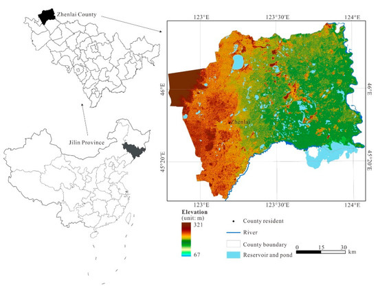
Figure 1.
The location of the study area.
The agricultural development in Zhenlai County is relatively delayed and is in the agro-pastoral transition zone of northern China. The ecological environment is fragile and extremely sensitive to human activities and climate change. Ecological problems, such as soil erosion, land desertification, and salinization occur frequently, severely restricting the sustainable development of the local socioeconomic and ecological environment. The historical process of human activities in the study area is the joint development of animal husbandry and planting from animal husbandry to form an agro-pastoral ecotone in space. From the 1980s to 2010, the arable land has been increasing year by year. Grassland, forestland, and wetland have been decreasing year by year. After 2010, by returning farmland to forestland and wetland, the growth trend of arable land basically stopped. Grassland, forestland, and wetland showed restorative growth. There is a detailed approach to the land use categories in Zhenlai in Table 1 and Table 2.

Table 1.
Detailed manner of the land use categories in Zhenlai (1986–2005).

Table 2.
Detailed manner of the land use categories in Zhenlai (2008–2013).
2.2. Data Sources
The years of 1986, 2000, 2005, 2008, 2010, and 2013 are used in this study. Landsat images composed the remote sensing information, and all of the remote sensing images were downloaded from the United States Geological Survey (USGS, http://www.usgs.gov). The LU spatial data were acquired using a manual interpretation. Based on the local characteristics and LU classification system in China, the LU was divided into seven types: arable land, forestland, grassland, water, settlements, wetlands, and other unused lands (including sandy land, saline-alkaline soil, and bare land).
The 30-m digital elevation model (DEM) data used in this study were the ASTER GDEM data and the surface information, such as the slope and aspect acquired using the surface tool in ArcGIS 10.2. The topographic data were from a 1:200,000 map of Baicheng City (1986), and the soil data were from a 1:200,000 map of the soil types in Jilin Province. Please refer to Appendix B for the soil and topographic types.
Relevant studies have shown that the most important natural driver that affects the LUCC is the soil, followed by the slope and elevation. Due to the small spatial differences in the climate factors at the county scale, the climate factors were not included as impact factors of LU suitability, and five natural geographic environmental factors, including the soil type, topographic type, elevation, slope, and aspect, as well as the distance to the rivers, were included [21,22]. The step of variable selection is realized in the deep learning iterative process.
Considering the interaction between the LU system and human activities, using the data of the LU types over the 6 years (1986 to 2013), the distance to the settlements and the distance to the roads were obtained using the Near tool in the software ARCGIS (ESRI, Redlands, CA, USA) [21,22,23,24].
2.3. Methods
The DLURM can perform LUCC reconstruction in terms of the time, location, and quantity. Based on historical data and big data of geography, and taking the grid as the unit, the DLURM combined the deep learning model to fit the drivers and mechanisms of LUCC, thereby successfully simulating the quantity and spatiotemporal distribution of LUCC.
2.3.1. Theoretical Basis
Because the LU process is constantly changing, it is impossible to completely determine its spatiotemporal conditions from the current situation. In the reconstruction of historical LUCC, limited by the lack of historical data and lack of LUCC information in historical data, reconstruction inaccuracy is inevitable. LUCC prediction is a study that provides the possibility of LUCC evolution based on the constraint conditions. All of the above studies are about uncertain problems, which must be supported by uncertainty reasoning [25].
Uncertainty reasoning refers to reasoning that is based on uncertain knowledge and evidence. It is an essential feature in the development and implementation of intelligent systems. Uncertainty reasoning is an important means for addressing the fragility of knowledge and the monotonicity of reasoning in traditional expert systems.
In the reconstruction of uncertainty information, modeling is one of the most effective techniques for studying the spatiotemporal process of LUCC. Constructing the spatiotemporal evolution model of LUCC can thoroughly and quantitatively explain the causes and processes of LUCC and identify the drivers and mechanisms of LUCC to summarize the spatiotemporal rules of LUCC. With the input of natural, social, and economic factors, the coupling mechanism can be analyzed, the history and current conditions can be clarified, and the future land development trends and their impacts on the environment can be predicted [26,27,28,29].
The DLURM can be regarded as a process that performs classification on the entire grid, classifying each unit (square or rectangle) of the grid. After the laws of the regional LUC are fully understood and the natural, social, and economic drivers on the LU system are considered, the probability of each LU type in the unit is calculated to determine which LU type is most likely to occur in the unit, and the LU type with the highest probability of occurrence is used to express the LU condition in the unit. In this way, the spatial reconstruction model of the LU should have high reliability and strong explanatory power (Figure 2).
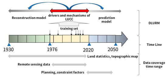
Figure 2.
Deep learning-integrated LUCC reconstruction model (DLURM) mechanism.
2.3.2. Modeling Framework
The DLURM consists of three main modules: the pre-reconstruction module (PM), deep learning module (DM), and spatial allocation module (SM) (Figure 3):
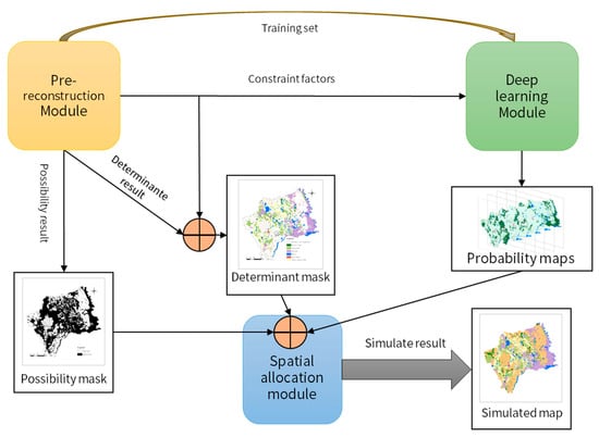
Figure 3.
DLURM modeling framework.
(1) PM: The PM is a process of information collection and collation and data preprocessing. It is the foundation and preparation stage of LUCC reconstruction. (2) DM: A deep learning algorithm is assembled to calculate the probability of each LU type in each grid unit. Through the analysis of the relationships between the LU distribution and various natural environmental and socioeconomic conditions, the evaluation maps of LU suitability, i.e., probability maps are drawn to show the possible spatial distribution of the land cover. (3) SM: According to certain principles or methods, the quantity of each LU in the geographical locations and spatially analytical outcomes is distributed. Then, the backward projection of the historical LU is realized. For the specific spatial allocation, under the control of the total land cover area and other distribution factors, the allocation can be performed in descending order based on the probability maps.
The classification and processing of the information and data is an important feature of the DLURM with the following characteristics:
Training set: The information in each grid unit contains the LU type and natural geographical attributes and human geographical attributes of itself and the neighboring grid units and is the database for obtaining the drivers and mechanisms of LUCC in the DM.
Constraint factors: These are the constraint conditions for generating the probability maps and are a prerequisite for spatial reconstruction. These factors include the quantity control of each LU type and the spatial distribution of the restricted LU types.
Determination result: This result is a collection of grid units that contains information about the time, location, and quantity. It is not an accurate result; therefore, the choice between quantity and accuracy is especially important. The determinant result can be described as the determinant mask.
Possibility result: Some grids can only contain the possibility information, which can be used to determine the LU type. The possibility result can be described as the possibility mask.
Simulated map: The selected masks are used to mask the probability maps (all or part) to control the area in or process of the image processing. Under the rule of spatial allocation, the simulated map is the optimal solution for the LUCC spatial distribution.
2.3.3. Deep Learning Model
Models based on artificial neural networks (ANNs), i.e., deep learning-based models, are gaining attention in the remote sensing domain [30,31,32,33,34]. The neural networks are used to fit the drivers and mechanisms of the LUCC. The drivers and mechanisms of the LUCC greatly influence the LUCC trajectories, play a dominant role in the study of the LUCC mechanism, and are the forces that cause changes in the LU patterns.
Currently, the drivers of LUCC often include natural, socioeconomic, and political factors. The current consensus is that natural conditions control the basic trends and processes of the overall LUCC and the changes in the natural environment, such as climate change, and change the spatial distribution pattern of LU to a great extent. Human activities and socioeconomic factors are the main drivers of LUCC on a small spatiotemporal scale. LUCC is mainly driven by socioeconomic factors over short periods, such as several years or decades. Political factors have a macro-control role in LU and its changes [35,36,37,38].
Traditional means and algorithms lack the ability to quantitatively analyze the drivers and mechanisms of LUCC, and the accumulation of massive data over the years provides the possibility of using deep learning models for related explorations. The probability of the LU distribution can be determined by a deep learning model. The LU probability cannot determine whether a certain LU type exists at that time; its function is to determine the distribution probability of a variety of LU types in a spatial unit, and the probability is the basis for the SM.
Figure 4 introduces the adopted DM. In the DM, the grid with the neighborhood features includes the LU type, soil, topography, elevation, slope, aspect, and distance-based variables, and all grid units are input into the DM in series. The deep learning method can model complex spatiotemporal dependencies, fit the drivers and mechanisms of the LUCC, derive the probability maps needed for the SM, and perform further LU simulations.
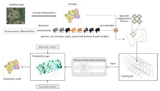
Figure 4.
Deep learning module.
A multilayer perceptron (MLP) is also known as an ANN. In addition to the input/output layer, it can have multiple hidden layers in between. The simplest MLP contains only one hidden layer, i.e., a total of three layers, and its structure is shown in Figure 5. The MLP has full connections between the layers. The bottom layer of the MLP is the input layer, the middle layer is the hidden layer, and the top layer is the output layer. Assuming that the input layer is denoted by the vector X, then the output of the hidden layer is f (W1X + b1), where W1 is the weight and b1 is the offset. The commonly used functions (f) include the sigmoid function, tanh function, ReLU function, among others.
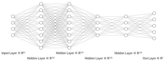
Figure 5.
Network structure.
The activation function used in this paper is the sigmoid function, and its mathematical form is shown below. In the domain, the activation function is a continuous, smooth, and differentiable function. Therefore, the sigmoid function can generate the output value of the network in the interval [0, 1], which is convenient for forward propagation.
Input Data
In this paper, the input data are 40-dimensional data. Due to the large time span and large land area in the training data, there are large differences in the distribution between different batches of training data in the training stage, and there is a certain distribution difference between the training set and the test set. Therefore, batch normalization is performed on the input data, where the specific calculation/transformation of BatchNorm (Algorithm 1) is shown below. First, the mean of each channel in the current batch is calculated, and then, the variance of each channel in the current batch is calculated. The mean is subtracted from the input, and the result is divided by the standard deviation to obtain the normalized output ; then, is multiplied by the scale parameter , and the shift parameter is added to obtain the final output :
| Algorithm 1. Batch normalizing transform applied to the activation x over a mini-batch. |
| Input: Values of x over a mini-batch: β = {}; Parameters to be learned: γ, β Output: { = } //mini-batch mean //mini-batch variance //normalize //scale and shift |
Network Structure
We conducted experiments on LUCC reconstruction in 2013 and 1980, and the overall accuracy rates were 91.2%, 91.8%, 92.3%, 92.1%, and 91.9% in 4–8 layers of neural networks, respectively. In this paper, the 6-layer neural network is adopted. The network structure is as follows (Figure 5): the number of neurons in each of the 6 layers is 40, 256, 256, 128, 128, and 5. The activation function used in this paper is the sigmoid function, which is a continuous and smooth function in the domain of definition, and it is differentiable everywhere. Therefore, the sigmoid function can compress the output value of the network to the interval [0,1], which is convenient for forward transmission. The output is the probability that the grid corresponds to the land use type, and the output of all of the grid units is combined to generate a probability map.
The data of a certain year are used as the test set, and the remaining data are the training and validation set. The training and validation set ia divided into ten parts using the 10-fold cross-validation method, in which nine of the parts are used as a training set and one is used for the validation set. The percentage of the training, validation, and testing sets is 5.4:0.6:1. The training set is the data sample used for model fitting. The validation set is a set of samples set aside separately during the model training. It can be used to adjust the hyperparameters of the model and to conduct a preliminary evaluation of the model’s capabilities. The testing set is used to evaluate the generalization ability of the final model. However, it cannot be used as a basis for algorithm-related selection such as parameter tuning and selection of features. The mean value of the ten results is used to estimate the accuracy of the algorithm in such a way that more accurate model results can be obtained.
Good performance on the training set, poor performance on the test set, and high variance are a sign of overfitting. To prevent overfitting of the model, the regularization method is used, and the dropout operation is added during the training stage. The neural network model of the dropout is shown in Figure 6. In this paper, the 6th layer dropout rate is 0.1, and for the other layers, it is 0.
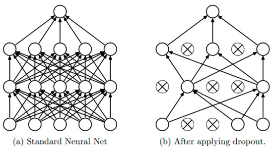
Figure 6.
Neural network model of dropout.
Left: standard neural network with 2 hidden layers.
Right: An example of a refined network generated by applying dropout to the network on the left. The cross symbol indicates that this unit is not activated. When training the neural network, some neurons in the neural network can be deleted, as shown in the figure, but all of the neurons should be activated during the test.
In the model training, the cross-entropy is used as the loss function, and the Adam optimization algorithm is used to update the weights of the neural network.
Because there are different numbers of samples of the five types of LU suitability samples in the training data, with a ratio of 7:14:1:5:7, there is an imbalance in the categorical data. In the training process, a relatively large weight is generated for the categories that have fewer samples, and a small weight is generated for the categories that have more samples, which solves the problem of the performance of the model being poor for the categories that have small sample sizes.
2.4. Reconstruction Procedure
In the following, the LUCC reconstruction of Zhenlai County in 2000 is used as an example to present the DLURM reconstruction process (the data of the year 2000 should be removed from the training set).
The natural and human geographical attributes of each grid unit (the soil, topography, elevation, slope, aspect, distance to settlements, distance to roads, and distance to rivers) (Figure 7) cover this grid unit and the neighboring units (8 × 5), with a total of 40 attributes.
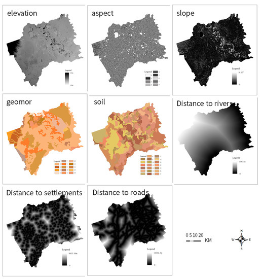
Figure 7.
Visualization of natural and human geographical attributes.
2.4.1. Pre-Reconstruction Module
The relevant settings (Figure 8) are as follows:
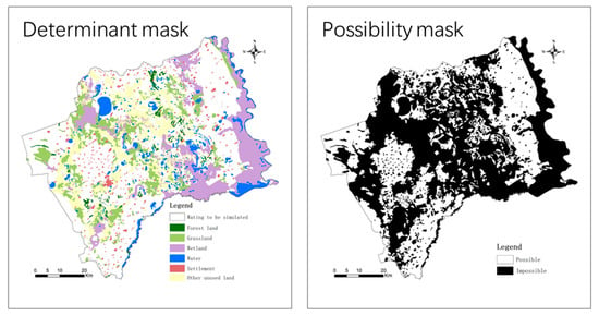
Figure 8.
Determinant mask and Possibility mask.
- (1)
- Determinant mask: The current LU spatial pattern dynamically depends on the historical spatial pattern, while the unchanged LU types in other years existed in 2000.
- (2)
- Possibility mask: For the LU types with human activities, such as arable land, the boundaries of one LU type in the past cannot exceed the boundaries of that LU type at the study time.
- (3)
- Training set: grid with neighborhood features of six years (1986, 2005, 2008, 2010, and 2013). The features include the LU type, soil, topography, elevation, slope, aspect, distance to settlements, distance to roads, distance to rivers in this grid unit, and the 4 neighborhood grid units.
- (4)
- Constraint Factors: The statistical data and the quantity simulated by the backtracking of the Markov model are combined, and the numbers of different LU types in 2000 after modification by the simulation numbers are as follows (Table 1):
2.4.2. Deep Learning Module
Probability maps (Figure 9): Water and settlements are constraint factors and can be determined by manual interpretation, and thus, no simulation is needed.
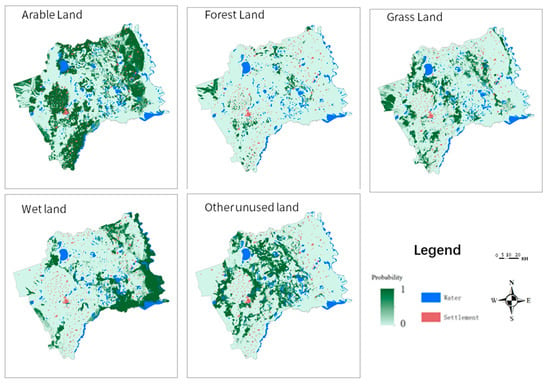
Figure 9.
Probability maps.
2.4.3. Spatial Allocation Module
According to the order of arable land, forestland, grassland, wetland, and other unused lands, under the quantitative control determined in the constraint factors and within the scope of the possibility factors, the LU type must be selected according to the positive order in the probability maps.
3. Results and Discussion
3.1. Competing Methods
Model validation usually requires a comparative analysis of the model simulation results and actual observation results (Figure 10).
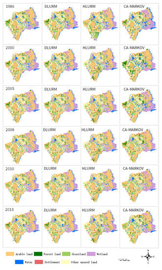
Figure 10.
Land use/cover change (LUCC) historical reconstructions through DLURM, historical land use reconstruction model (HLURM), and cellular automata (CA)-Markov models.
To evaluate the accuracy and performance of the DLURM, comparisons with the CA-Markov model and HLURM are introduced. The HLURM is an excellent integrated model that has been published and widely recognized. It represents the level of current mature models [17], thus, a comparison with the HLURM is introduced. The software IDRISI Selva (17.02) is used for the CA-Markov simulation.
Table 3 lists the reconstruction results using the DLURM, HLURM, and CA-Markov model in the test set (1986, 2000, 2005, 2008, 2010, and 2013).

Table 3.
Overall accuracy.
Table 3 shows that compared with those of the HLURM and CA-Markov model, the DLURM has significantly better overall accuracy for the reconstruction results, with an overall accuracy increase of 9.66% and 6.89%, respectively, i.e., the error rate decreases by 57.53% and 49.14%, respectively. The DLURM is significantly better than the other two traditional models.
Another standard method for the evaluation of the accuracy of the LUCC simulation, the three-map comparison method, is also used to evaluate the DLURM.
This method superimposes the simulated maps and reference maps to determine the quantity and spatial allocation of the errors in the simulated maps. This method reveals the accuracy of the model by comparing it with the null model (model with no changes at all). See Appendix A for details.
Table 4 lists the evaluation results of the DLURM, HLURM, and the CA-Markov model based on the three-map comparison method, and the test sets of 1986, 2000, 2005, 2008, 2010, and 2013 are used (Figure 11). (Explanation of hit, miss, false alarms, and null success classes: (1) hits: A certain pixel is predicted to be changed and in fact is changed; (2) misses: A certain pixel is predicted to be unchanged but in fact is changed; (3) false alarms: A certain pixel is predicted to be changed but in fact is not changed; (4) null successes: also known as correct rejections, a certain pixel is predicted to be unchanged and in fact is not changed in both simulated and reference LUC maps).

Table 4.
Prediction correctness and error (Appendix A).
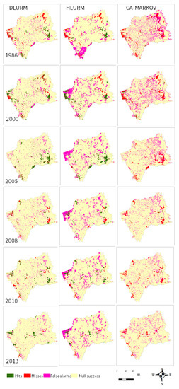
Figure 11.
Prediction correctness and error.
The DLURM and HLURM are significantly better than CA-Markov in terms of hits. The DLURM is the best in terms of overall accuracy and has high robustness. Figure 12 shows the differences between the simulation results of all of the reconstruction models in one randomly selected region. As shown in the figure, the simulation results of the proposed DLURM can better match the actual LU map than the other models.
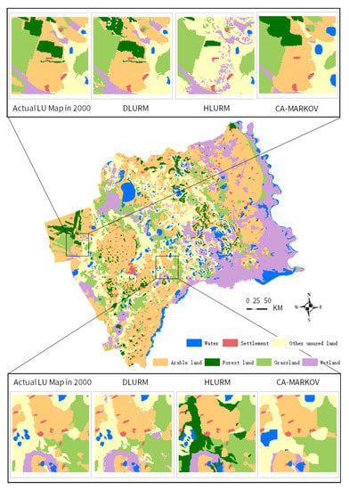
Figure 12.
Comparison of simulated results for 2000, using several models of the study area.
3.2. Reconstruction of the LUCC Dataset of Zhenlai County from 2000 to 2019
In recent years, automatic and semiautomatic interpretation has developed rapidly, and cartographic efficiency has been improved each year compared with the original methods, which can meet the requirements for generating products of large-scale land classification data. However, the accuracy of the interpretation is usually between 70% and 90%, the accuracy rates of various LU types differ significantly, and the accuracy of the supervised classification widely used in the industry is less than 80%. At present, the accuracy of manual interpretation/HCI interpretation is the highest, and the average accuracy in this paper reaches 92.9%. However, the labor and time costs of manual interpretation are too high, which makes it difficult to realize a year-by-year interpretation of a large geographical area [39,40,41,42,43,44,45,46,47].
This study realizes a year-by-year interpretation in a short time with high accuracy, as demonstrated by the data of 2000–2019. Figure 13 shows the 30 m × 30 m LUCC dataset of Zhenlai County reconstructed by the DLURM from 2000 to 2019 (for 2000, 2005, 2008, 2010, 2013, and 2015, manual interpretation was performed).
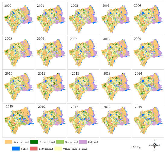
Figure 13.
2000–2019 LUCC reconstructions.
4. Discussion
The main applications of the DLURM are historical LUCC reconstructions in the years without remote sensing images and future LUCC predictions. We compared the DLURM results with other previous studies on the same topic:
Zhenlai County, China was selected in this study, and the performance of the proposed DLURM was validated by comparing the DLURM to the HLURM and CA-Markov model. The experimental results showed that the DLURM had a significantly better overall accuracy of the reconstruction, reaching 92.87%. Compared with the results of the traditional models, the overall accuracy of the DLURM model improved by 9.66% and 6.89%, i.e., the error rate decreased by 57.53% and 49.14%, respectively.
The DLURM had high robustness. Compared with the simulation results of the HLURM and CA-Markov model, the spatial distribution of LUCC based on the DLURM can better match the actual LU spatial distribution.
Through the high-resolution reconstruction of LUCC in Zhenlai County from 2000 to 2019, we found that the study area is located in the semi-humid and semi-arid plain area in the western part of Northeast China. The growth rate of arable land slowed down from 1980 to 2010, and the growth sources were grassland and wetland. The urbanization process is accelerating, and the settlement is growing. Since 2010, China has vigorously conducted the construction of ecological civilization. With the implementation of the ecological restoration project of returning farmland to forestland and wetland, the amount of forestland has increased year by year, and the grassland, woodland, and wetland have been restored.
Work that can be further conducted in the future includes the following:
- (1)
- There is still room for optimization and improvement of the deep learning model. Long short-term memory (LSTM) [48,49,50] can be introduced to accurately capture the long-term spatiotemporal dependence and thus obtain more accurate LUCC predictions.
- (2)
- Future studies should use high-resolution datasets, consider various drivers, such as land-use policies, population density, space, and geophysical and socioeconomic factors, and analyze the impacts of different factors.
- (3)
- The LUCC reconstruction and prediction in areas with large spatiotemporal ranges and different ecogeographical features can be studied. The future work plan is to reconstruct and predict the LUCC of Northeast China from 1950 to 2050 through the DLURM to investigate the spatiotemporal evolution pattern.
- (4)
- Expanding the range of the adjacent grids to 64 × 64 or 256 × 256 can be considered, and a convolution neural network can be used to capture the potential spatial elements to completely represent the neighborhood effects. Through comparisons, the choice between multi-area modeling or holistic modeling in a large spatiotemporal range can be determined.
5. Conclusions
Overall, the main novelty of this paper can be summarized as follows:
- (1)
- In this paper, a novel model that integrates deep learning for LUCC reconstruction, namely, the DLURM, was proposed. This model can learn the long-term spatiotemporal distribution pattern of LUCC and capture the potential spatial characteristics of the neighborhoods by using historical multiperiod LUCC data sets interpreted with HCI to effectively represent the neighborhood effect.
- (2)
- Compared with traditional models, the HLURM and CA-Markov model, the DLURM had higher performance, higher robustness, and a better match to the actual LU spatial distribution. Taking Zhenlai County as an example, this paper used a novel model that integrates deep learning for LUCC reconstruction, i.e., the DLURM, to reconstruct the year-by-year LUCC information from 2000 to 2019. [51,52,53,54]. The DLURM provides tools for long-term high-resolution LUCC reconstruction.
- (3)
- The DLURM is customizable and has a high degree of freedom and strong scalability. In addition, it is based on multi-source data and interdisciplinary reconstruction. In related research, different data sources are fused to obtain more information about LUCC. LUCC reconstruction can complement different perspectives and verify the reconstruction results so as to improve the reconstruction accuracy. In summary, the fusion of different methods and data sources can increase the information about environmental change in a large space-time scale.
Author Contributions
Conceptualization, Z.Y. (Zhang Yubo); Data curation, Z.Y. (Zhang Yubo) and Y.Z.; Formal analysis, Z.Y. (Zhang Yubo); Investigation, Z.Y. (Zhang Yubo) and C.L.; Methodology, Z.Y. (Zhang Yubo); Resources, Z.Y. (Zhang Yubo) and Y.Y.; Software, Z.Y. (Zhang Yubo); Validation, Z.Y. (Zhang Yubo); Visualization, Z.Y. (Zhang Yubo) and Z.Y. (Zhang Yucong); Writing—original draft, Z.Y. (Zhang Yubo), Y.L.; Writing—review and editing, Z.Y. (Zhang Yubo), Y.J., W.D., Y.F. and Z.S. All authors have read and agreed to the published version of the manuscript.
Funding
This research was funded by the National Key Research and Development Project (No. 2017YFC0504202) and the Strategic Priority Research Program of the Chinese Academy of Sciences (No. XDA2003020103; XDA23060405).
Acknowledgments
The authors would like to thank the anonymous members for their helpful comments on the primary version of the manuscripts.
Conflicts of Interest
The authors declare no conflict of interest.
Appendix A
Pontius et al. [55], García et al. [56], and Chen proposed a standard method to assess the accuracy of LUC simulation, the three-map comparison method. This method superimposes the simulated maps and reference maps to determine the quantity and spatial allocation errors of the simulated maps. It reveals the accuracy of the model by comparing it with the null model (model with no changes at all [55,56,57]).
This method must compare three LU maps to validate the LUC model, i.e., the reference map at the simulation start time point (t1), the reference map at the simulation end time point (t2), and the simulated map at t2. Through the superposition of the reference map at t1 and the reference map at t2, the observed LUC map, i.e., the reference LUC map, can be obtained, which reflects the actual dynamic LUC. Through the superimposition of the reference map at t1 and the simulated map at t2, the simulated LUC information, i.e., the simulated LUC map can be obtained, which reflects the simulation behavior of the model. This validation method allows us to understand the consistency (or error) between the simulated LUC map and the reference LUC map (actual LU type map). Through a comparison of the simulated LUC map and reference LUC map, the accuracy of the model can be determined by four indexes that indicate whether the pixel change is correct or not: hits, misses, false alarms, and null successes.
Based on these four indexes, a series of validation indexes are proposed, such as the error due to quantity (EQ, Equation (A4)), error due to allocation (EA, Equation (A5)), and figure of merit (FOM, Equation (A1)), to measure the simulation accuracy. The EQ reflects the errors due to the inaccurate estimation of the net changes by the model, and this type of error is not caused by spatial allocation. The EA reflects the defects in the model in the process of allocating the changing pixels over the entire landscape, and this type of error originates from the spatial allocation process of the model; it is related to the independent variables used in the model and is very sensitive to the changes in the space allocation algorithms. In addition, the FOM (Equation (A1)) and the other three indexes (Equations (A2)–(A4)) that quantify the percentages of hits, misses, and false alarms are used to analyze the observed changes. This verification method is more realistic than the other methods, such as the kappa index and overall accuracy index, in evaluating the pixel-to-pixel consistency between the simulated and actual maps. The kappa index or the overall accuracy index applies to the whole study area [57]. The range of the FOM is 0–100%, in which 0% means that there is no overlap between the observed changes and predicted changes and 100% means that there is a complete overlap between the observed changes and predicted changes.
where H, M, and F represent the hits, misses, and false alarms, respectively; HOC, MOC, and FOC represent the percentages of hits, misses, and false alarms in the observed changes, respectively.
OC ≡ Observed Change = M + H
PC ≡ Predicted Change = H + F
T ≡ Total Error = M+F
EQ = |PC − OC| = |(H + F) − (M + H)| = |F − M|
EA = T − Q = (M + F) − |F − M| = 2 × Mininum(F,M)
Appendix B
The type of geomorphology is shown in Table A1.
The type of soil is shown in Table A2.

Table A1.
Type of geomorphology.
Table A1.
Type of geomorphology.
| Code | Geomorphology | Code | Geomorphology |
|---|---|---|---|
| 0 | Low altitude semifixed grass shrub stone | 10 | Low-altitude higher terraces of rivers |
| 1 | Low-altitude semifixed gently undulating sand | 11 | Low-altitude lacustrine alluvial lower terraces |
| 2 | Low-altitude alluvial floodplain | 12 | Low-altitude lacustrine alluvial plain |
| 3 | Low-altitude alluvial pluvial low platform | 13 | Low-altitude lacustrine lower terraces |
| 4 | Low-altitude alluvial pluvial high platform | 14 | Low-altitude lacustrine higher terraces |
| 5 | Low-altitude alluvial lacustrine plain | 15 | Low-altitude lacustrine plain |
| 6 | Low-altitude alluvial plain | 16 | Low-altitude lakeshore |
| 7 | Low-altitude alluvial-fan plain | 17 | Low-altitude erosion denuded low platform |
| 8 | Low-altitude fixed and gently undulating sand | 18 | Lake |
| 9 | Low-altitude lower terraces of rivers | 19 | Low-altitude erosion denuded low hills |

Table A2.
Type of soil.
Table A2.
Type of soil.
| Code | Soil | Code | Soil |
|---|---|---|---|
| 0 | planosol | 14 | glen meadow soil |
| 1 | dark chernozem | 15 | salinized meadow soil with soda |
| 2 | chernozem | 16 | ±soda meadow saline soils + meadow alkali soil |
| 3 | light chernozem | 17 | meadow marsh soil |
| 4 | light chernozem + meadow alkali soil | 18 | humus marsh soil |
| 5 | meadow chernozem | 19 | peat soil |
| 6 | carbonate chernozem | 20 | alluvial soil |
| 7 | dark chestnut soil | 21 | meadow saline soil |
| 8 | meadow dark chestnut soil | 22 | soda meadow saline soil + meadow alkali soil |
| 9 | meadow soil | 23 | meadow alkali soil |
| 10 | dark meadow soil | 24 | meadow alkali soil + soda meadow saline soils |
| 11 | carbonate meadow soil | 25 | grass wind sandy soil |
| 12 | carbonate meadow soil + meadow alkali soil | 26 | meadow aeolian sandy soil |
| 13 | albic meadow soil | 27 | water |
References
- Fu, P.; Weng, Q.H. A time series analysis of urbanization induced land. use and land cover change and its impact on land surface temperature with Landsat imagery. Remote Sens. Environ. 2016, 175, 205–214. [Google Scholar] [CrossRef]
- Lyu, R.; Clarke, K.C.; Zhang, J.; Jia, X.; Feng, J.; Li, J. The impact of urbanization and climate change on ecosystem services: A case study of the city belt along the Yellow River in Ningxia, China. Comput. Environ. Urban Syst. 2019, 77, 101351. [Google Scholar] [CrossRef]
- Lambin, E.F. Modelling and monitoring land-cover change processes in tropical regions. Prog. Phys. Geogr. 1997, 21, 375–393. [Google Scholar] [CrossRef]
- Turner Ii, B.L.; Lambin, E.F.; Reenberg, A. The emergence of land change science for global environmental change and sustainability. Proc. Natl. Acad. Sci. USA 2007, 104, 20666–20671. [Google Scholar] [CrossRef]
- Foster, D.; Swanson, F.; Aber, J.; Burke, I.; Brokaw, N.; Tilman, D.; Knapp, A. The importance of land-use legacies to ecology and conservation. Bioscience 2003, 53, 77–88. [Google Scholar] [CrossRef]
- Gragson, T.L.; Bolstad, P.V. Land use legacies and the future of southern Appalachia. Soc. Nat. Resour. 2006, 19, 175–190. [Google Scholar] [CrossRef]
- Lambin, E.F.; Turner, B.L.; Geist, H.J.; Agbola, S.B.; Angelsen, A.; Bruce, J.W.; Coomes, O.T.; Dirzo, R.; Fischer, G.; Folke, C.; et al. The causes of land-use and land-cover change: Moving beyond the myths. Glob. Environ. Change-Hum. Policy Dimens. 2001, 11, 261–269. [Google Scholar] [CrossRef]
- Yang, Y.; Zhang, S.; Yang, J.; Xing, X.; Wang, D. Using a cellular automata-markov model to reconstruct spatial land-use patterns in Zhenlai county, Northeast China. Energies 2015, 8, 3882–3902. [Google Scholar] [CrossRef]
- Garosi, Y.; Sheklabadi, M.; Conoscenti, C.; Pourghasemi, H.R.; Van Oost, K. Assessing the performance of GIS- based machine learning models with different accuracy measures for determining susceptibility to gully erosion. Sci. Total Environ. 2019, 664, 1117–1132. [Google Scholar] [CrossRef]
- Griffiths, P.; Nendel, C.; Hostert, P. Intra-annual reflectance composites from Sentinel-2 and Landsat for national-scale crop and land cover mapping. Remote Sens. Environ. 2019, 220, 135–151. [Google Scholar] [CrossRef]
- Han, W.; Feng, R.; Wang, L.; Cheng, Y. A semi-supervised generative framework with deep learning features for high-resolution remote sensing image scene classification. ISPRS J. Photogramm. Remote Sens. 2018, 145, 23–43. [Google Scholar] [CrossRef]
- Heipke, C.; Rottensteiner, F. Deep learning for geometric and semantic tasks in photogrammetry and remote sensing. Geo-Spat. Inf. Sci. 2020, 23, 10–19. [Google Scholar] [CrossRef]
- Horning, N.; Fleishman, E.; Ersts, P.J.; Fogarty, F.A.; Wohlfeil Zillig, M.; Pettorelli, N.; Disney, M. Mapping of land cover with open-source software and ultra-high-resolution imagery acquired with unmanned aerial vehicles. Remote Sens. Ecol. Conserv. 2020. [Google Scholar] [CrossRef]
- Yang, Y.; Liu, Y.; Xu, D.; Zhang, S. Use of intensity analysis to measure land use changes from 1932 to 2005 in Zhenlai county, Northeast China. Chin. Geogr. Sci. 2017, 27, 441–455. [Google Scholar] [CrossRef]
- Yang, Y.; Zhang, S. Historical arable land change in an eco-fragile area: A case study in Zhenlai county, Northeastern China. Sustainability 2018, 10, 3940. [Google Scholar] [CrossRef]
- Yang, Y.; Zhang, S.; Yang, J.; Chang, L.; Bu, K.; Xing, X. A review of historical reconstruction methods of land use/land cover. J. Geogr. Sci. 2014, 24, 746–766. [Google Scholar] [CrossRef]
- Yang, Y.; Zhang, S.; Liu, Y.; Xing, X.; de Sherbinin, A. Analyzing historical land use changes using a historical land use reconstruction model: A case study in Zhenlai county, northeastern China. Sci. Rep. 2017, 7, 41275. [Google Scholar] [CrossRef]
- Abdi, A.M. Land cover and land use classification performance of machine learning algorithms in a boreal landscape using Sentinel-2 data. GIScience Remote Sens. 2019, 57, 1–20. [Google Scholar] [CrossRef]
- Aung, S.W.Y.; Khaing, S.S.; Aung, S.T. Multi-label land cover indices classification of satellite images using deep learning. In Big Data Analysis and Deep Learning Applications. ICBDL 2018. Advances in Intelligent Systems and Computing; Zin, T., Lin, J.W., Eds.; Springer: Singapore, 2019; pp. 94–103. [Google Scholar]
- Flynn, T.; Rozanov, A.; de Clercq, W.; Warr, B.; Clarke, C. Semi-automatic disaggregation of a national resource inventory into a farm-scale soil depth class map. Geoderma 2019, 337, 1136–1145. [Google Scholar] [CrossRef]
- Bai, S.Y.; Zhang, S.W.; Zhang, Y.Z. Correlation analysis on the arable land distribution and changes. Chin. J. Soil Sci. 2005, 36, 652–654. [Google Scholar] [CrossRef]
- Bu, K.; Zhang, S.W.; Zhang, Y.Z.; Wang, W.J.; Zhang, Y.B. The Effect of Soil Types on the Process of Farmland in Sanjiang Plain in Recent 50 Year. Resour. Sci. 2008, 30, 702–708. [Google Scholar] [CrossRef]
- Liu, M.; Zhao, C.W.; Shi, M.H. Spatial autocorrelation analysis of multi-scale land use change at mountainous areas in Guizhou province. Trans. Chin. Soc. Agric. Eng. 2012, 20, 239–246. [Google Scholar] [CrossRef]
- Lin, Q.; Luo, G.P.; Chen, X. Review of Land-use Model. Prog. Geogr. 2005, 24, 79–87. [Google Scholar] [CrossRef]
- Bai, S.Y.; Zhang, S.W. The Discussion of the Method of Land Utilization Spatial Information Reappearance of History Period. J. Arid Land Resour. Environ. 2004, 18, 77–80. [Google Scholar] [CrossRef]
- Li, Z.T.; Li, M.; Xia, B.C. Spatio-temporal dynamics of ecological security pattern of the Pearl River Delta urban agglomeration based on LUCC simulation. Ecol. Indic. 2020, 114, 106319. [Google Scholar] [CrossRef]
- Li, C.; Zhang, Y.; Shen, Y.; Kong, D.; Zhou, X. LUCC-driven changes in gross primary production and actual evapotranspiration in Northern China. J. Geophys. Res. Atmos. 2020, 125, e2019JD031705. [Google Scholar] [CrossRef]
- Colné, J.; Conart, J.B.; Luc, A.; Perrenot, C.; Berrod, J.P.; Angioi-Duprez, K. Simulateur de chirurgie de cataracte EyeSi: Validité de construction des modules capsulorhexis, phacoémulsification et aspiration des masses cristalliniennes. J. Fr. Ophtalmol. 2019, 42, 49–56. [Google Scholar] [CrossRef]
- Li, K.; Feng, M.; Biswas, A.; Su, H.; Niu, Y.; Cao, J. Driving factors and future prediction of land use and cover change based on satellite remote sensing data by the LCM model: A case study from Gansu Province, China. Sensors 2020, 20, 2757. [Google Scholar] [CrossRef]
- Ienco, D.; Interdonato, R.; Gaetano, R.; Ho Tong Minh, D. Combining sentinel-1 and sentinel-2 satellite image time series for land cover mapping via a multi-source deep learning architecture. ISPRS J. Photogramm. Remote Sens. 2019, 158, 11–22. [Google Scholar] [CrossRef]
- Zhang, L.; Zhang, L.; Du, B. Deep learning for remote sensing data: A technical tutorial on the state of the art. IEEE Geosci. Remote Sens. Mag. 2016, 4, 22–40. [Google Scholar] [CrossRef]
- Kussul, N.; Lavreniuk, M.; Skakun, S.; Shelestov, A. Deep learning classification of land cover and crop types using remote sensing data. IEEE Geosci. Remote Sens. Lett. 2017, 14, 778–782. [Google Scholar] [CrossRef]
- Lyu, H.B.; Lu, H.; Mou, L.C. Learning a transferable change rule from a recurrent neural network for land cover change detection. Remote Sens. 2016, 8, 506. [Google Scholar] [CrossRef]
- Zhu, X.X.; Tuia, D.; Mou, L.; Xia, G.; Zhang, L.; Xu, F.; Fraundorfer, F. Deep learning in remote sensing: A comprehensive review and list of resources. IEEE Geosci. Remote Sens. Mag. 2017, 5, 8–36. [Google Scholar] [CrossRef]
- Shao, Z.; Cai, J.; Fu, P.; Hu, L.; Liu, T. Deep learning-based fusion of landsat-8 and sentinel-2 images for a harmonized surface reflectance product. Remote Sens. Environ. 2019, 235, 111425. [Google Scholar] [CrossRef]
- Zhang, C.; Sargent, I.; Pan, X.; Li, H.; Gardiner, A.; Hare, J.; Atkinson, P.M. Joint deep learning for land cover and land use classification. Remote Sens. Environ. 2019, 221, 173–187. [Google Scholar] [CrossRef]
- Zhong, L.; Hu, L.; Zhou, H. Deep learning based multi-temporal crop classification. Remote Sens. Environ. 2019, 221, 430–443. [Google Scholar] [CrossRef]
- Zhong, L.; Hu, L.; Zhou, H.; Tao, X. Deep learning based winter wheat mapping using statistical data as ground references in Kansas and northern Texas, US. Remote Sens. Environ. 2019, 233, 111411. [Google Scholar] [CrossRef]
- Liu, J.; Tian, H.; Liu, M.; Zhuang, D.; Melillo, J.M.; Zhang, Z. China’s changing landscape during the 1990s: Large-scale land transformations estimated with satellite data. Geophys. Res. Lett. 2005, 32, L02405. [Google Scholar] [CrossRef]
- Churches, C.E.; Wampler, P.J.; Sun, W.; Smith, A.J. Evaluation of forest cover estimates for Haiti using supervised classification of Landsat data. Int. J. Appl. Earth Obs. Geoinf. 2014, 30, 203–216. [Google Scholar] [CrossRef]
- Liu, J.; Liu, M.; Tian, H.; Zhuang, D.; Zhang, Z.; Zhang, W.; Tang, X.; Deng, X. Spatial and temporal patterns of China’s cropland during 1990–2000: An analysis based on Landsat TM data. Remote Sens. Environ. 2005, 98, 442–456. [Google Scholar] [CrossRef]
- Liu, J.Y.; Zhang, Z.X.; Xu, X.L.; Kuang, W.H.; Zhou, W.C.; Zhang, S.W.; Li, R.D.; Yan, C.Z.; Yu, D.S.; Wu, S.X.; et al. Spatial patterns and driving forces of land use change in China during the early 21st century. J. Geogr. Sci. 2010, 20, 483–494. [Google Scholar] [CrossRef]
- Bodart, C.; Eva, H.; Beuchle, R.; Raši, R.; Simonetti, D.; Stibig, H.J.; Brink, A.; Lindquist, E.; Achard, F. Pre-processing of a sample of multi-scene and multi-date Landsat imagery used to monitor forest cover changes over the tropics. ISPRS J. Photogramm. Remote Sens. 2011, 66, 555–563. [Google Scholar] [CrossRef]
- Rogan, J.; Franklin, J.; Roberts, D.A. A comparison of methods for monitoring multitemporal vegetation change using Thematic Mapper imagery. Remote Sens. Environ. 2002, 80, 143–156. [Google Scholar] [CrossRef]
- Glanz, H.; Carvalho, L.; Sulla-Menashe, D.; Friedl, M.A. A parametric model for classifying land cover and evaluating training data based on multi-temporal remote sensing data. ISPRS J. Photogramm. Remote Sens. 2014, 97, 219–228. [Google Scholar] [CrossRef]
- Tang, J.; Chen, F.; Schwartz, S.S. Assessing spatiotemporal variations of greenness in the Baltimore–Washington corridor area. Landsc. Urban Plan. 2012, 105, 296–306. [Google Scholar] [CrossRef]
- Kontgis, C.; Schneider, A.; Ozdogan, M. Mapping rice paddy extent and intensification in the Vietnamese Mekong River Delta with dense time stacks of Landsat data. Remote Sens. Environ. 2015, 169, 255–269. [Google Scholar] [CrossRef]
- Xing, W.; Qian, Y.; Guan, X.; Yang, T.; Wu, H. A novel cellular automata model integrated with deep learning for dynamic spatio-temporal land use change simulation. Comput. Geosci. 2020, 137, 104430. [Google Scholar] [CrossRef]
- Wang, Y.; Li, S. Simulating multiple class urban land-use/cover changes by RBFN-based CA model. Comput. Geosci. 2011, 37, 111–121. [Google Scholar] [CrossRef]
- Wu, H.; Lin, A.; Zhou, J.; Li, Z.; Clarke, K.C.; Shi, W.; Fang, L. Examining the sensitivity of spatial scale in cellular automata Markov chain simulation of land use change. Int. J. Geogr. Inf. Sci. 2019, 33, 1040–1061. [Google Scholar] [CrossRef]
- Fuchs, R.; Herold, M.; Verburg, P.H.; Clevers, J.G.; Eberle, J. Gross changes in reconstructions of historic land cover/use for Europe between 1900 and 2010. Glob. Chang. Biol. 2015, 21, 299–313. [Google Scholar] [CrossRef]
- Fuchs, R.; Herold, M.; Verburg, P.H.; Clevers, J.G.P.W. A high-resolution and harmonized model approach for reconstructing and analysing historic land changes in Europe. Biogeosciences 2013, 10, 1543–1559. [Google Scholar] [CrossRef]
- Fuchs, R.; Verburg, P.H.; Clevers, J.G.P.W.; Herold, M. The potential of old maps and encyclopaedias for reconstructing historic European land cover/use change. Appl. Geogr. 2015, 59, 43–55. [Google Scholar] [CrossRef]
- Verburg, P.H.; Overmars, K.P. Combining top-down and bottom-up dynamics in land use modeling: Exploring the future of abandoned farmlands in Europe with the Dyna-CLUE model. Landsc. Ecol. 2009, 24, 1167–1181. [Google Scholar] [CrossRef]
- Pontius, R.G.; Boersma, W.; Castella, J.C.; Clarke, K.; de Nijs, T.; Dietzel, C.; Duan, Z.; Fotsing, E.; Goldstein, N.; Kok, K.; et al. Comparing the input, output, and validation maps for several models of land change. Ann. Reg. Sci. 2008, 42, 11–37. [Google Scholar] [CrossRef]
- García, A.M.; Santé, I.; Boullón, M.; Crecente, R. A comparative analysis of cellular automata models for simulation of small urban areas in Galicia, NW Spain. Comput. Environ. Urban Syst. 2012, 36, 291–301. [Google Scholar] [CrossRef]
- Chen, H.; Pontius, R.G. Diagnostic tools to evaluate a spatial land change projection along a gradient of an explanatory variable. Landsc. Ecol. 2010, 25, 1319–1331. [Google Scholar] [CrossRef]
© 2020 by the authors. Licensee MDPI, Basel, Switzerland. This article is an open access article distributed under the terms and conditions of the Creative Commons Attribution (CC BY) license (http://creativecommons.org/licenses/by/4.0/).