Article

Assessment of Cornfield LAI Retrieved from Multi-Source Satellite Data Using Continuous Field LAI Measurements Based on a Wireless Sensor Network

1
State Key Laboratory of Remote Sensing Science, Jointly Sponsored by Beijing Normal University and Institute of Remote Sensing and Digital Earth of Chinese Academy of Sciences, Beijing 100875, China
2
Beijing Engineering Research Center for Global Land Remote Sensing Products, Institute of Remote Sensing Science and Engineering, Faculty of Geographical Science, Beijing Normal University, Beijing 100875, China
3
Ottawa Research and Development Centre, Agriculture and Agri-Food Canada, Ottawa, ON K1A 0C6, Canada
4
Institute of Geography, Fujian Normal University, Fuzhou 350007, China
5
Beijing XiaoBaiShiJi Network Technical Co., Ltd., Beijing 100084, China
6
Heihe Remote Sensing Experimental Research Station, Key Laboratory of Remote Sensing of Gansu Province, Northwest Institute of Eco-environment and Resources, CAS, Lanzhou 730000, China
7
CAS Center for Excellence in Tibetan Plateau Earth Sciences, Chinese Academy of Sciences (CAS), Beijing 100101, China
8
Northwest Institute of Eco-Environment and Resources, Chinese Academy of Sciences (CAS), Lanzhou 730000, China
*
Author to whom correspondence should be addressed.
Remote Sens. 2020, 12(20), 3304; https://doi.org/10.3390/rs12203304
Submission received: 4 September 2020 / Revised: 8 October 2020 / Accepted: 9 October 2020 / Published: 11 October 2020

Abstract

:
Accurate and continuous monitoring of leaf area index (LAI), a widely-used vegetation structural parameter, is crucial to characterize crop growth conditions and forecast crop yield. Meanwhile, advancements in collecting field LAI measurements have provided strong support for validating remote-sensing-derived LAI. This paper evaluates the performance of LAI retrieval from multi-source, remotely sensed data through comparisons with continuous field LAI measurements. Firstly, field LAI was measured continuously over periods of time in 2018 and 2019 using LAINet, a continuous LAI measurement system deployed using wireless sensor network (WSN) technology, over an agricultural region located at the Heihe watershed at northwestern China. Then, cloud-free images from optical satellite sensors, including Landsat 7 the Enhanced Thematic Mapper Plus (ETM+), Landsat 8 the Operational Land Imager (OLI), and Sentinel-2A/B Multispectral Instrument (MSI), were collected to derive LAI through inversion of the PROSAIL radiation transfer model using a look-up-table (LUT) approach. Finally, field LAI data were used to validate the multi-temporal LAI retrieved from remote-sensing data acquired by different satellite sensors. The results indicate that good accuracy was obtained using different inversion strategies for each sensor, while Green Chlorophyll Index (CIgreen) and a combination of three red-edge bands perform better for Landsat 7/8 and Sentinel-2 LAI inversion, respectively. Furthermore, the estimated LAI has good consistency with in situ measurements at vegetative stage (coefficient of determination R2 = 0.74, and root mean square error RMSE = 0.53 m2 m−2). At the reproductive stage, a significant underestimation was found (R2 = 0.41, and 0.89 m2 m−2 in terms of RMSE). This study suggests that time-series LAI can be retrieved from multi-source satellite data through model inversion, and the LAINet instrument could be used as a low-cost tool to provide continuous field LAI measurements to support LAI retrieval.

1. Introduction

Leaf area index (LAI) of terrestrial vegetation is a widely used vegetation structural parameter, defined as one half the total leaf area per unit ground area [1,2]. It is a crucial driving factor for climate, hydrology, biogeochemistry, and ecology in ecosystem process-based models [3]. It has been considered as one of the key biophysical parameters among eighteen terrestrial Essential Climate Variables (ECVs) by the Global Climate Observing System (GCOS) community [4]. Due to the temporal variation in LAI throughout the growing season, accurate estimation of the seasonal dynamics of LAI is of great importance to precision agriculture (e.g., above-ground biomass estimation [5]) and model-driven scientific research [6,7].
LAI can be measured in situ using hand-held instruments or estimated from remote-sensing date acquired by various sensors. A wide-range of field LAI measuring methods and instruments are available [8]. While direct methods (e.g., harvesting leaves and measuring leaf area using the LI-3000 portable leaf area meter) are desirable as they measure true LAI (LAIt), indirect methods to derive effective LAI (LAIe) have also been widely used due to their high efficiency. In particular, the development of automated ground LAI measurement technology makes it more convenient to collect time-series LAI. For example, LAINet is an emerging indirect tool to collect LAI automatically at fixed positions continuously based on a WSN technology [9,10]. It consists of four components, including an above-canopy node, a below-canopy node, a central node, and a solar power supply system. Precisely, LAINet can measure the effective Plant Area Index (PAIe) from multi-point directional transmittance based on the Beer-Lambert Law, as the sensors do not discriminate leaves with different chlorophyll contents from other plant tissues [9]. Other similar automated LAI measurement methods, such as the PAI Autonomous System from Transmittance Instantaneous Sensors at 57° (PASTIS-57) instrument [11,12], automated digital hemispherical photography (DHP) [13,14], automated digital cover photography [15], and terrestrial laser scanning [16] have been developed.
LAI estimation from remote-sensing data has unique advantages in terms of large spatial coverage and continuous temporal resolution compared with field LAI measurement. During the last two decades, two primary types of methods have been used to derive LAI from high-resolution satellite data: (1) empirical/semi-empirical methods; (2) physical methods based on radiative transfer modelling (RTM), e.g., the combined PROSPECT leaf optical properties model and SAIL canopy bidirectional reflectance model (i.e., PROSAIL [17,18,19]), or the Discrete Anisotropic Radiative Transfer model (DART) [20]. Compared with the statistical method, the physical method is more generic for deriving LAIs of different vegetation types with fewer field LAI measurements [17]. However, the inversion of an RTM is an “ill-posed” process, as LAI is only one of the variables affecting canopy reflectance. Various approaches have been proposed to deal with this issue, e.g., the look-up tables, machine learning [21], data assimilation [22], and incorporation of a prior knowledge. Errors can be introduced by uncertainties in the reflectance data through modeling and inversion algorithms [23]. The discrepancy and uncertainty of LAI derived from remote-sensing inversion should be further evaluated.
The validation of remote-sensing LAI estimates is an independent process to help diagnose algorithm deficiencies, understand error sources, and further improve the accuracy of LAI products [24]. In this context, field LAI measurements are usually used as a benchmark. However, due to a scale mismatch, discrepancies between field LAI measurements and pixel values in LAI products pose a challenge to operational applications [23,25]. The Committee on Earth Observation Satellites (CEOS) Land Product Validation (LPV) subgroup proposed a “bottom-up” validation framework [26], which is internationally recognized and widely used [27]. Following this framework, to quantify the uncertainties of global LAI products, such as the Moderate Resolution Imaging Spectroradiometer (MODIS LAI) [3], the Visible Infrared Imager Radiometer Suite (VIIRS) LAI [28], the Global Land Surface Satellite (GLASS) LAI [29], and the Copernicus Global Land Service LAI [30], more systematic in situ LAI measurements are needed over time and across space. Meanwhile, due to the universality of spatial heterogeneity, representative and spatially intensive sampling is necessary to measure LAI, which can increase the cost of human labor for ground data collection using hand-held instruments. At this point, automated LAI instruments with acceptable accuracy can substantially reduce the costs of field LAI collection.
Besides, high-quality satellite images with fine spatial and temporal resolution are useful to up-scale field LAI measurements to match with moderate (0.1–1 km) and coarse resolution (>1 km) LAI products. Currently, decametric-resolution optical image data from a single-satellite sensor are limited in temporal resolution. For example, the Landsat time-series images with a 16-day repeat cycle are not able to provide near-real-time crop phenology and dynamic monitoring, and this can become worse when there is cloud interference or other unfavorable weather conditions such as rain and haze. With finer spatial and temporal resolution, Sentinel-2A/B satellites are promising but are still affected by cloud interference. Hence, it is difficult to acquire enough high-quality images from a single high-resolution satellite to capture the temporal variability of LAI throughout the growing season. While data fusion approaches were used to generate daily and gap-free images at a finer spatial resolution [31], it is difficult to quantify the uncertainty induced by the fusing algorithms. A simple combination of multi-source RS data from different satellite sensors remains a direct option. This requires consistent LAI retrievals from different satellite sensors with high quality.
The goal of this study is to evaluate LAI retrievals from multi-source satellite data using ground LAI measurements acquired by LAINet. The specific objectives are to (1) evaluate the stability and accuracy of LAINet measurements; (2) estimate LAI from Landsat 7/8 and Sentinel-2 data through inversion of the PROSAIL model; and (3) assess the difference between LAI inversion and field measurement during the whole growing season of corn.

2. Materials and Methods

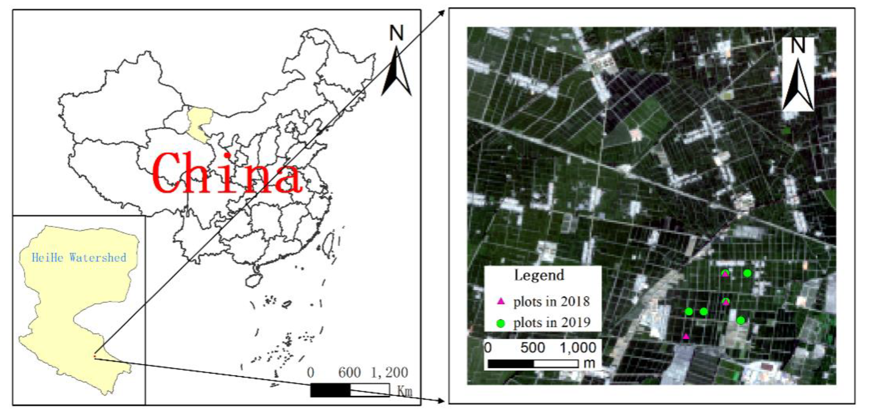
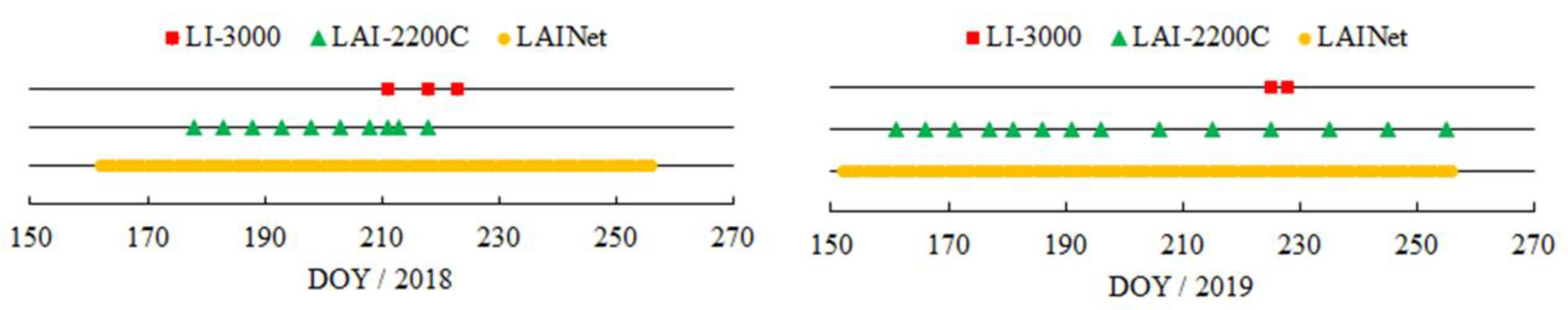
2.1. Study Area and Field Data Collection

The study site is approximately 4 × 4 km, located in the middle reach of the Heihe watershed, an artificial oasis in northwest China (38°80′N, 100°40′E). The area is relatively flat with an average elevation of 1556 m. It belongs to the cold arid climate according to the Köben-Geiger climate classification [32,33]. The average annual temperature and precipitation are 6~8 °C and 140 mm, respectively. Corn is planted at the end of April and harvested in mid-September. Figure 1 shows the location of the study area and the spatial distribution of field observation plots.
In situ LAI was measured from June 11 to September 13 in 2018, and from June 1 to September 13 in 2019. LAI was measured using three instruments, LAINet, LAI-2200C plant canopy analyzer, and LI-3000. The frequency of measurements is shown in Figure 2. LAINet measurements were used for evaluating LAI retrievals from RS images. The algorithm to derive in situ LAI from LAINet measurements is briefly introduced in Section 2.3, and more detailed information can be found in Qu et al., 2014 [9]. In 2018, three 30 × 30 m corn plots were selected. In each plot, five nodes installed understory were deployed to measure the transmitted solar radiation, and one above-canopy node was fixed on a flux tower nearby to measure the incoming solar radiation after DOY 192. Before this, one above-canopy node was deployed per plot. In 2019, six 30 × 30 m corn plots were selected, with four below-canopy nodes and one above-canopy node per plot. The LAINet datasets of both years have been released publicly via the National Science & Technology Infrastructure (http://www.tpdc.ac.cn/zh-hans/, in Chinese). Measurements corresponding to each below-canopy node were obtained from LAI-2200C. For LAINet and LAI-2200C, field LAI measurements within a plot were averaged to represent the plot LAI. Destructive LAI was measured using LI-3000 from three corn plants per plot.

2.2. Remote-Sensing Data

The satellite data used in this study were acquired by Landsat 7 the Enhanced Thematic Mapper Plus (ETM+) (Level-2), Landsat 8 the Operational Land Imager (OLI) (Level-2), and Sentinel-2A/B Multispectral Instrument (MSI) (Level-1C) (Table 1).
Level-2 surface reflectance images acquired by ETM+ and OLI were downloaded from the United States Geological Survey (USGS) Land Product Characterization System (https://earthexplorer.usgs.gov/). The data have a spatial resolution of 30m in the Universal Transverse Mercator (UTM) projection. Both ETM+ and OLI have a similar band setting. No missing data were used in the Landsat ETM+ SLC−off product, as nothing was done to fill the gaps. The quality assessment values stored in the quality assessment band (BQA) were used for removing pixels influenced by cloud, and only pixels marked as clear terrain were selected. For Landsat 7, Band 2 (G: green, 0.519–0.601 nm), Band 3 (R: red, 0.631–0.692 nm), Band 4 (NIR: near-infrared, 0.772–0.898 nm), Band 5 (SWIR-1: shortwave infrared 1, 1.547–1.749 nm), and Band 6 (SWIR-2: shortwave infrared 2, 2.064–2.345 nm) were used for LAI retrieval. For Landsat 8, Band 3 (G: green, 0.533–0.590 nm), Band 4 (R: red, 0.636–0.673 nm), Band 5 (NIR: near-infrared, 0.851–0.879 nm), Band 6 (SWIR-1: shortwave infrared 1, 1.566–1.651 nm), and Band 7 (SWIR-2: shortwave infrared 2, 2.107 – 2.294 nm) were used for LAI retrieval. The blue band was excluded because of strong atmospheric interference in this band. In addition, three vegetation indices (VIs), including the normalized difference vegetation index (NDVI), the enhanced vegetation index (EVI2), and a chlorophyll index - Green (CIgreen) were also derived for inversion. NDVI was considered, as it has been widely used for estimating vegetation biophysical parameters [23,34,35]. Both EVI2 and CIgreen have a stronger correlation with LAI, especially when LAI is large [35]. The details on using these spectral bands and VIs are presented in methodology in Section 2.4.
Sentinel-2A/B Level-1C images were also obtained from the USGS website. The European Space Agency’s Sen2Cor V2.5.5, a specialized processor to perform atmospheric correction, was used to derive Level-2 surface reflectance [36]. Band 3 (G: green, central wavelength at 0.560 nm), Band 4 (R: red, 0.665 nm), Band 8 (NIR: near-infrared, 0.842 nm), Band 5 (red-edge 1, 705 nm), Band 6 (red-edge 2, 740 nm), and Band 7 (red-edge 3, 783 nm) were used in this study. All image bands were resampled to 20 m in UTM projection using the Sen2Cor tool. In addition to NDVI, EVI2, CIgreen, a chlorophyll index—Red-edge (CIred-edge) was derived for LAI estimation, because the red-edge index has been found to be more sensitive to LAI [35].

2.3. LAI Measurement Using LAINet

LAINet was calibrated using an integrating sphere in the laboratory before it was deployed in the fields. LAI is measured through its relationship with light transmission via the Beer-Lambert law
T ( θ , θ L )   =   e G ( θ L , θ ) LAI / cos ( θ )
where T is light transmission through the canopy, and is calculated as the ratio of solar downwelling radiation measured by below-canopy nodes to that measured by above-canopy nodes, G is the extinction coefficient, θ L is the leaf inclination angle, and θ is the solar zenith angle. Following the method in Demon instruments [37], Equation (1) can also be expressed as follows
T ( θ )   =   e 0 π / 2 A ( θ L , θ ) g ^ ( θ L ) LAI d θ L
where A ( θ L , θ ) is a trigonometric function, and g ^ ( θ L ) is a distribution function of θ L . The detailed algorithm principle of LAINet can be found in Qu, et al. [10,38]. The leaf inclination angle of corn can be represented by probability density function with a vertically dominated orientation of leaf tissues, with an average inclination angle of 63.2° [10,38].
LAINet measured multi-angle light transmittance through vegetation canopy during the day from 06:00 am to 18:30 pm on a daily basis, with a 10 min interval. All the measurements were used to estimate daily LAI. To reduce the error of daily LAI values introduced by weather conditions, LAINet measurements were smoothed using a 7-day moving window. Generally, a window of 3 to 8 days was acceptable to capture crop growth dynamics [38]. The performance of LAINet was evaluated by comparing its measurements with LAI measured by LAI-2200C and LI-3000. We characterized the measurement uncertainty of LAINet and LAI-2200C by relative predictive error (RPE) [39]
RPE = LAI indirect LAI Ref LAI Ref × 100 %
where LAI indirect represents LAI measured by LAINet and LAI-2200C, and LAI Ref represents LAI measured by LI-3000 as LAI true-values.

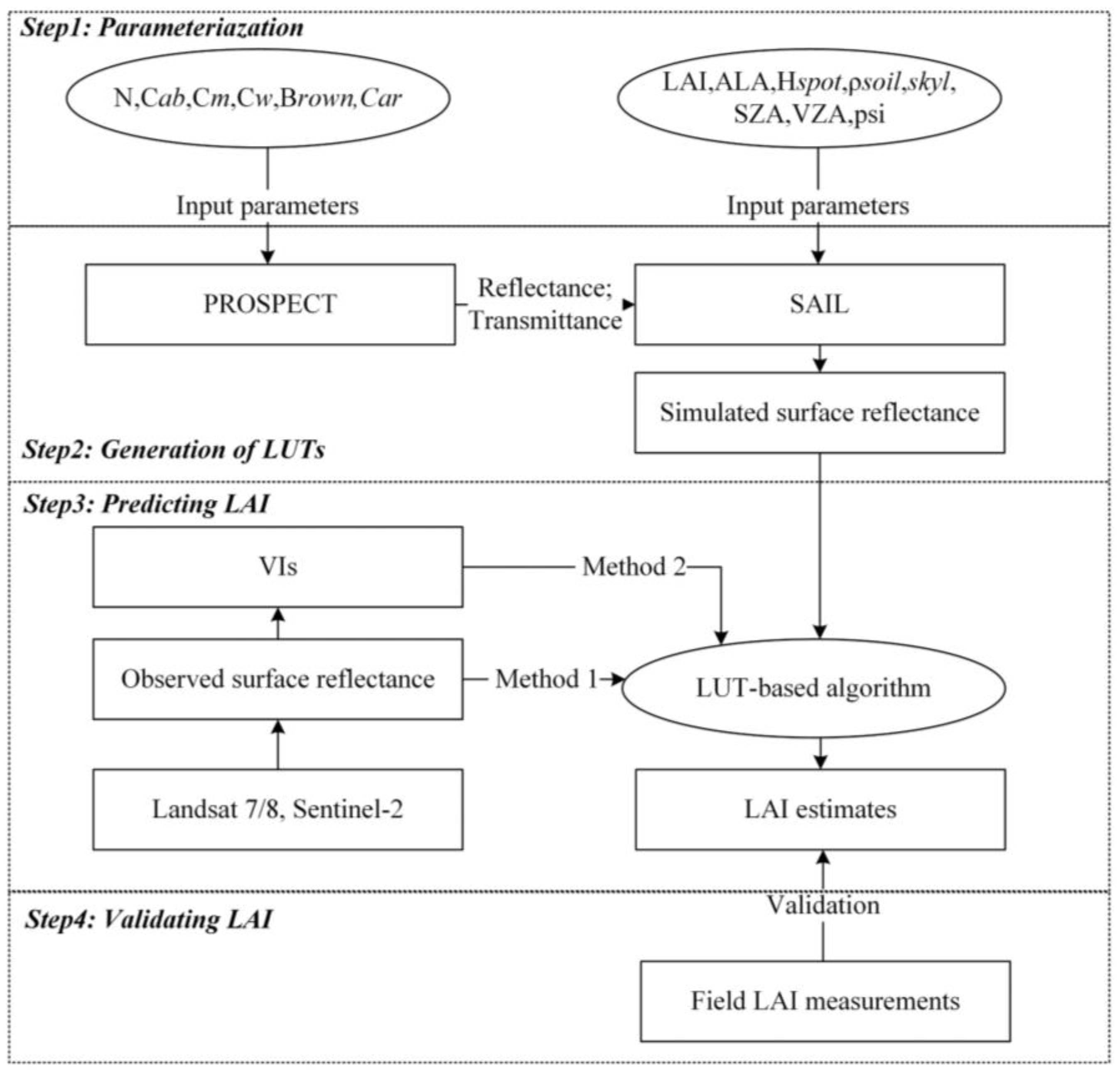
2.4. Estimation and Validation of LAI Retrieved from Remote-Sensing Data

Statistical methods based on regression functions are not general, and the model parameters should be recalibrated when the site and time change. Hence, the physical method using the PROSAIL model was applied to LAI inversion in this study. The PROSAIL model has been widely used to simulate canopy spectral reflectance in croplands and grassland [31]. It combines the SAIL canopy reflectance model and the PROSPECT leaf optical model. For the leaf model (PROSPECT 5), six leaf parameters are needed, which include leaf structural parameter (N), leaf chlorophyll content (Cab), equivalent water thickness (Cw), leaf dry matter content (Cm), brown pigment content (Brown), and carotenoid content (Car). For the canopy model (4SAIL), eight parameters are needed, which include leaf area index (LAI), average leaf angle (ALA), diffuse/total radiation (skyl), soil brightness coefficient ( ρ soil ), hot spot effect (Hspot), solar zenith angle (SZA), view zenith angle (VZA), and relative azimuth angle (psi) (see Table 2). The reflectance and transmittance of leaf simulated from PROSPECT are used as inputs into SAIL.
In this study, reflectance and VIs were employed separately to invert the PROSAIL model for LAI estimation. An LUT-based method was used to determine acceptable LAI solutions by matching the measured and simulated spectral reflectance or VI. Figure 3 shows the process flow of LAI estimation and validation from multi-source satellite data.
  • Step1: Parameterization of the PROSAIL model
Previous studies [40,41] showed that the reflectance at visible and NIR regions was weakly affected by Cm, N, and Cw but strongly influenced by ALA and LAI. Therefore, Cm, N, and Cw were generally given constant values [41]. In this study, the values and ranges of all parameters are listed in Table 2.
  • Step2: Creation of sensor-specific LUTs
Sensor-specific LUTs on reflectance were generated using the Latin hypercube sampling method. When given the ranges, probability distribution or sampling intervals of each of the sensitive parameters, the model obtains the reflectance values over a specific band. Canopy reflectance was determined with the leaf-level models (i.e., PROSPECT 5) and canopy-level models (i.e., SAIL). The process to generate an LUT is to run the forward PROSAIL model using given model parameters (Table 2). The total number of records simulated in an LUT was 100,000. For the convenience of LAI inversion at subsequent steps and computational efficiency, simulated reflectance stored in LUTs was resampled to Landsat 7/8 and Sentinel-2 bands based on their corresponding spectral response functions.
  • Step3: LAI estimation
Two strategies can be used for LAI estimation from an LUT. Method 1 is to match satellite-derived reflectance with simulated reflectance in the LUT in order to find corresponding parameters, e.g., LAI. For Landsat, four cases including single R, the combination of R and NIR, the combination of R, NIR, SWIR1 and SWIR 2, the combination of SWIR1 and SWIR 2, were used in the inversion. For Sentinel-2, four cases including single G, R and NIR, Red-edge1 and NIR, a combination of three Red-edge bands, were used in the inversion. Method 2 is to match VI derived from satellite data with VI derived from simulated reflectance in the LUT. Table 3 shows four VIs in this study, and the reasons for selecting these indices are presented in Section 2.2. By comparing accuracies of LAI retrieved from different VIs and reflectance, the VI or spectral bands with the best accuracy was selected for LAI estimation.
A simple cost function (CF) based on the Root Mean Square Error (RMSE) between simulations and observations was used to help obtain acceptable LAI solutions
CF Ref = 1 n i = 1 n ( Ref observed ( i ) Ref simulated ( i ) ) 2
CF VI = ( VI observed VI simulated ) 2
where n is the total number of bands used in the inversion (e.g., n = 2 for the combination of R and NIR bands ), Ref observed ( i ) is the satellite-observed reflectance of band i , Ref simulated ( i ) is the simulated reflectance of band i in an LUT, VI observed is the value of VI calculated from satellite-observed reflectance, VI simulated is the value of VI calculated from simulated reflectance in an LUT. Some studies suggested that the threshold of 10% was a good tradeoff between LAI accuracy and computing resources according to previous studies [31,45]. Some studies used threshold of less than 20% [46,47]. The selection of from 50 to 20% records is considered as a reasonable threshold range [31]. In this study, the first 100 records with the smallest CF values were selected, and the corresponding LAI values were averaged as estimated LAI [27].
  • Step4: Validation of LAI retrievals
The field LAI measured using LAINet was used to validate LAI retrievals. Referring to a previous study [9], LAINet data seem to be closer to LAIt, possibly due to the leaf angle distribution adopted in LAINet algorithm. LAINet data were further adjusted with a scaling factor of 1.3 in this study. A total of 104 samples from the two years were available for the evaluation of LAI retrievals, 16 for Landsat 8, 31 for Landsat 7, and 57 for Sentinel-2. Reflectance and VIs corresponding to each plot were derived from all satellite images. At each sample location, a 3 × 3 pixels window for Sentinel-2 and a 2 × 2 pixels window for Landsat 7/8 were used, and the average values were derived to reduce the potential geo-positioning errors. The RS-derived LAI were validated at the plot-scale using field LAI measurements collected by LAINet. Both the coefficient of determination (R2) and the root mean square error (RMSE) were used to quantify the performance and uncertainty of LAI estimates

3. Results

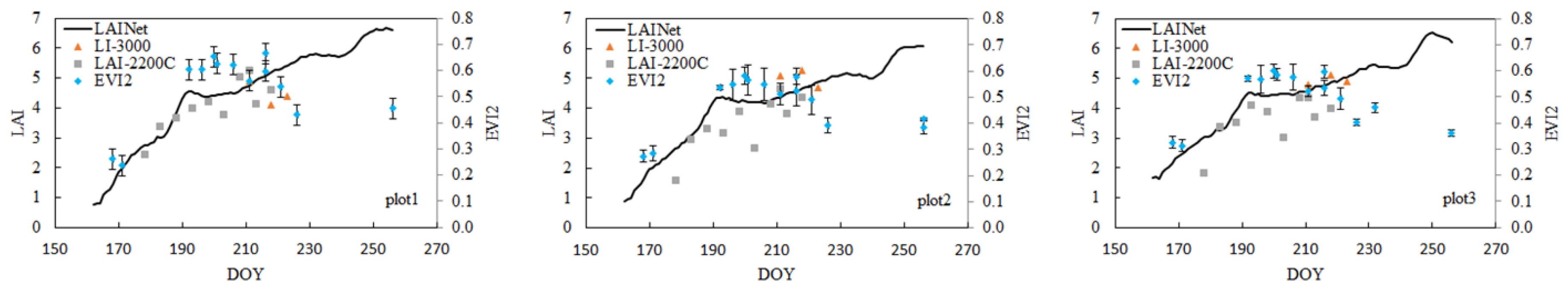
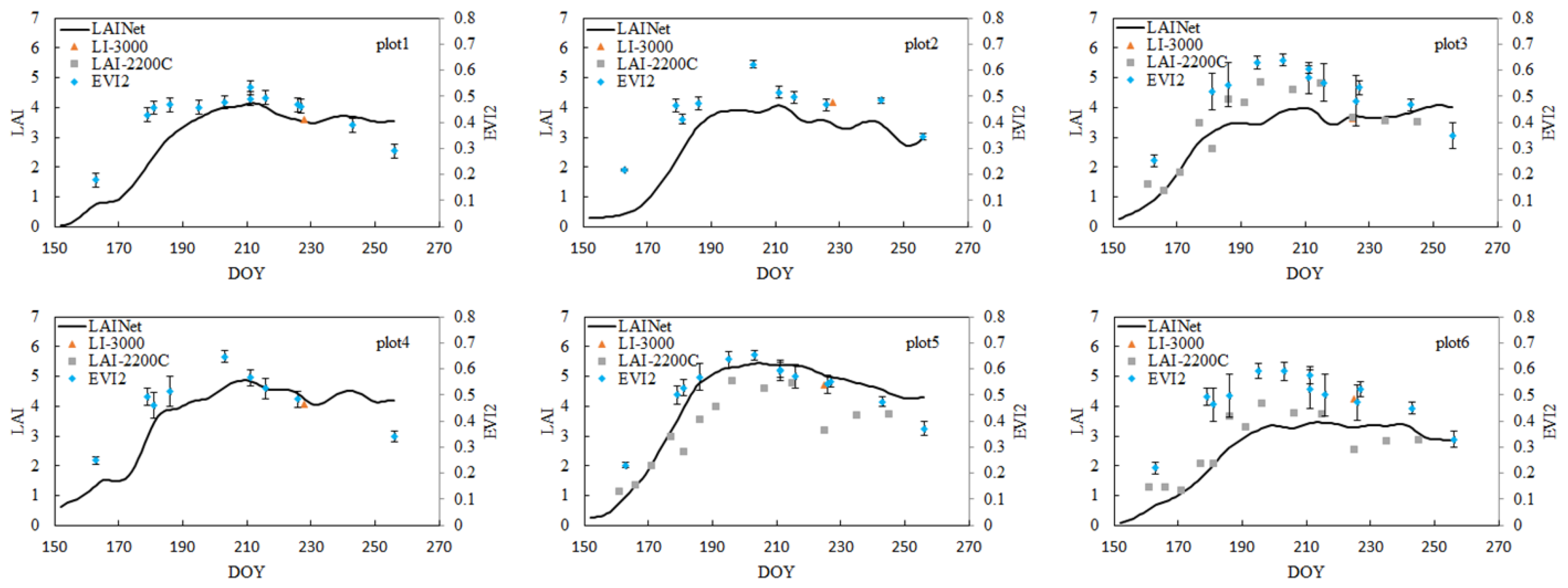
3.1. Seasonal Changes of Field LAI using LAINet

Seasonal variations of in situ LAI, as measured by LAINet, LAI-2200C, and LI-3000, are shown in Figure 4 for 2018 and Figure 5 for 2019. LAINet data shown in Figure 5 were smoothed with a moving window average algorithm. For both years, from June to September, LAI measured by LAINet ranged from 0.76 to 6.70 in 2018, and from 0.41 to 5.45 in 2019.
The dynamics of LAI for different corn plots measured by LAINet show similarity in the same year. A peak was found in the seasonal profile of measured LAI around DOY 192 in 2018. This was probably due to a change in the observation conditions of LAINet in the year, and weather conditions. The field deployment and installation of LAINet were improved in 2019. LAI measured in 2018 and 2019 show an opposite trend later in the season (after DOY around 212). LAI at the later season (after DOY around 212) shows an increased trend in 2018 (Figure 4) but a slightly declining trend in 2019 (Figure 5). To inspect this phenomenon, we compared the trends of LAINet to that of EVI2 derived from multiple RS images. The temporal variations in EVI2 and LAINet are also shown in Figure 4 and Figure 5. For both years, EVI2 showed a decreasing trend after DOY 212, in conformity with the trends of measured LAI using the LAINet in 2019. This shows a potential measurement issue during senescent stage in 2018. The relationship between LAINet measurements and EVI2 are shown by the scatterplot in Figure 6. The figure reveals that in 2018, EVI2 decreased when LAINet measurements increased beyond 3.5, whereas this was not the case in 2019. Based on the aforementioned analysis, the LAINet measurements in 2018 appeared to be subjected to an overestimation at the later stage. Thus, LAI measured during that period were not used in subsequent validation of the remote-sensing retrievals. As a result, two Sentinel-2 images acquired on 13 September 2018 (DOY 256) and 14 August (DOY 2213 September 2018Sep 13th 2018 and 11 July 2018 (DOY 192), were excluded.
LAI measured using LAI-2200C and LI-3000 on a few days in the two years generally followed the same trend as that measured using LAINet. There were three paired measurements (see Table 4) among three types of measurements on DOY 225 in 2019 to compute the RPE (see Equation (3)). LAI values from LAINet and LAI-2200C underestimated LAIt values with a mean RPE of 4.4% and 23.7%, respectively. According to the statistics, the averaged LAI from LAINet, LAI-2200C, and LI-3000 was 4.0, 3.1 and 4.2, respectively. Compared with measurement using LAI2200C, LAI derived from LAINet was more consistent with that of LI-3000. The ratio of averaged LAI value between LAINet (4.0) and LAI-2200C (3.1) was 1.3, which was used to adjust LAINet data so that measurements between the two sensors were consistent. After being adjusted, the absolute bias between LAINet and LAI-2200C decreased from 0.87 to 0.05.

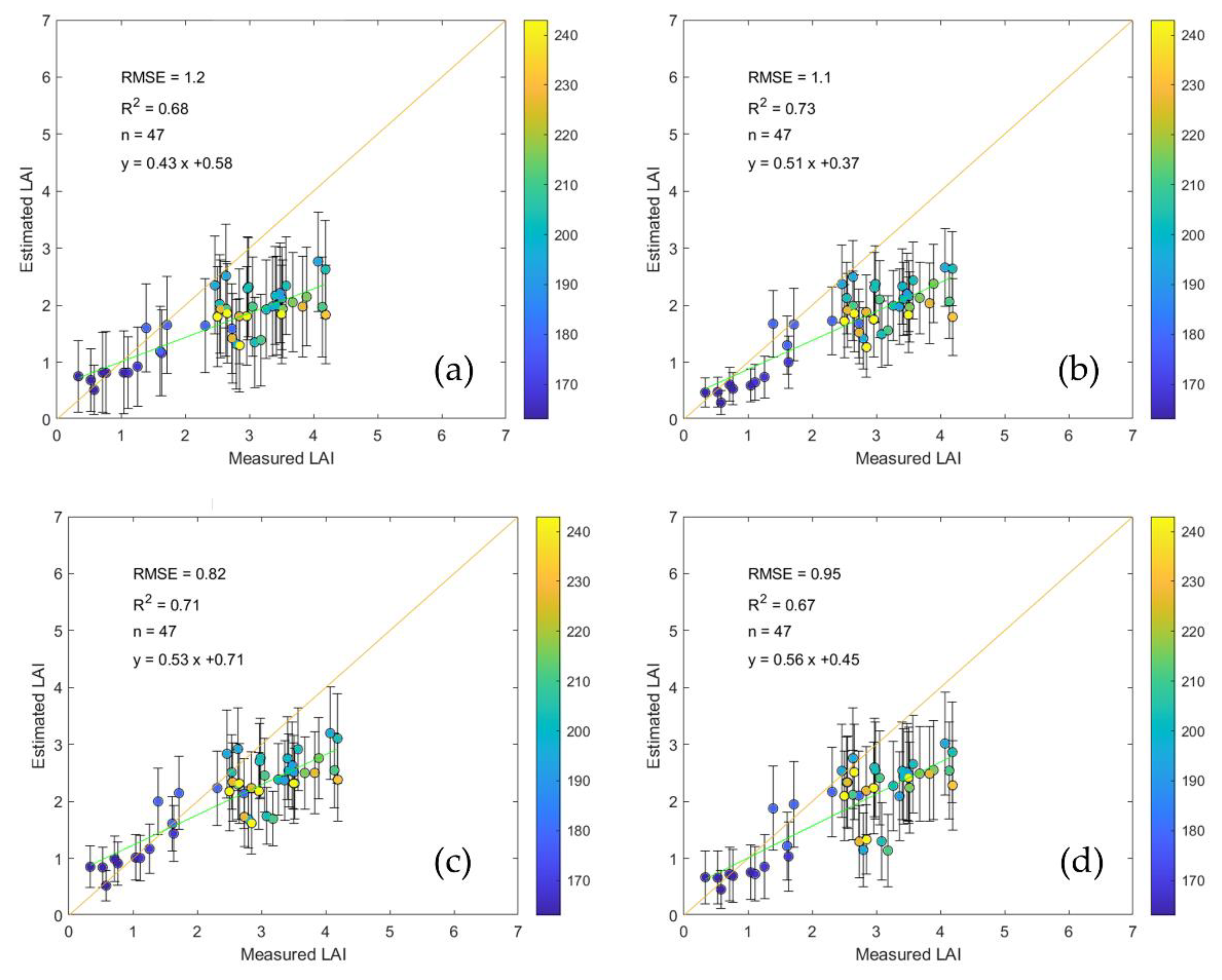
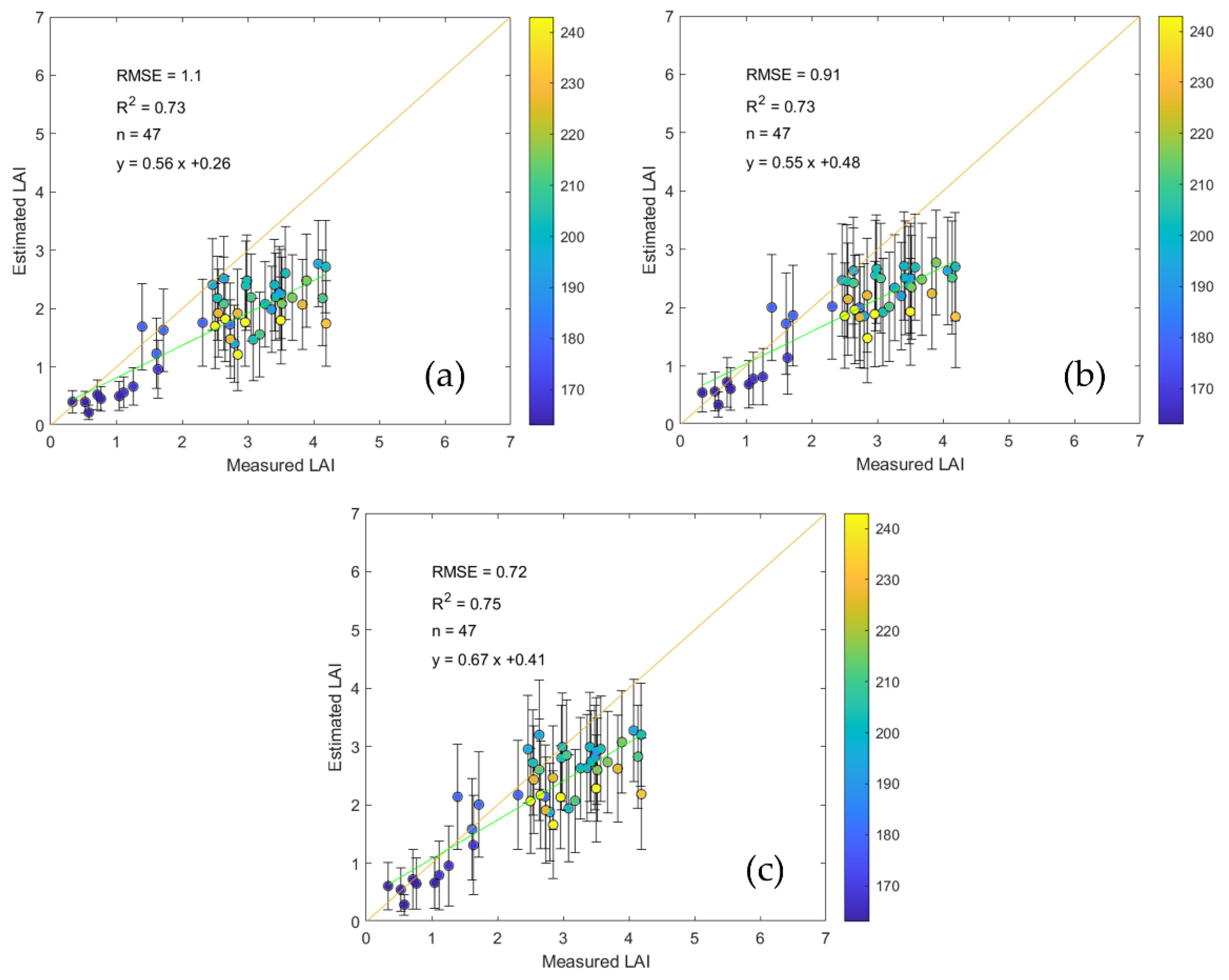
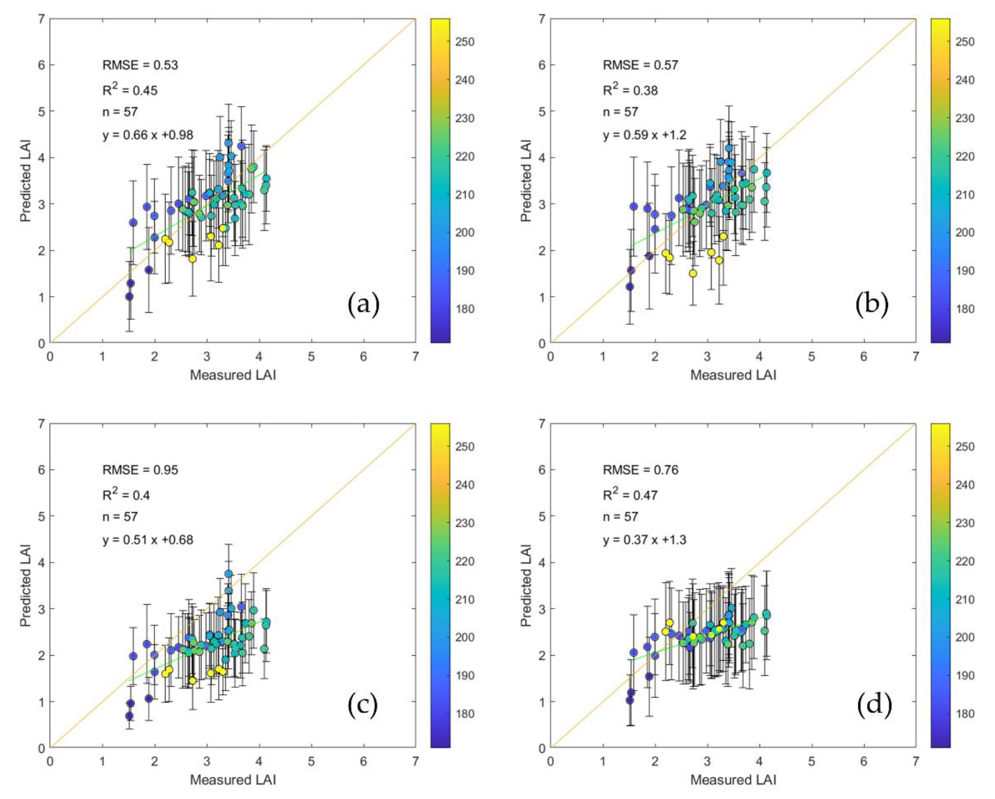
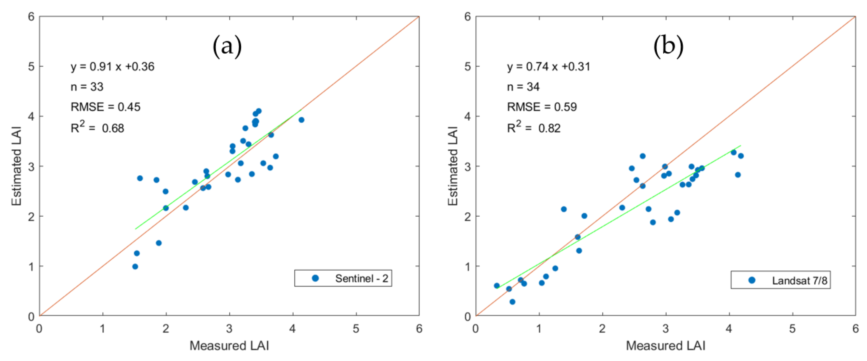
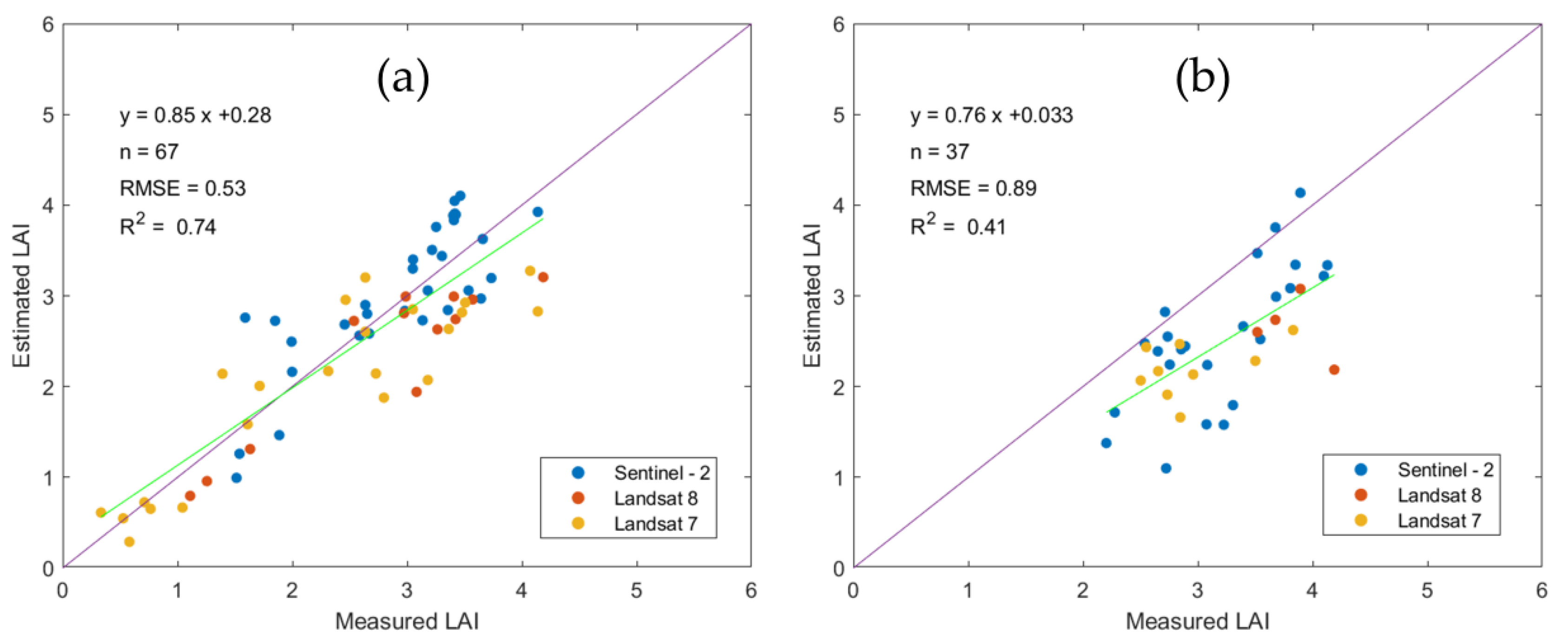
3.2. LAI Inversion from Landsat and Sentinel-2 Data

For Landsat data, four combinations of band reflectance and three VIs (see Table 3) were used to estimate LAI. Figure 7 shows the comparison of LAI retrieved from Landsat surface reflectance with that measured using LAINet. Among the four band combinations, the combination of R, NIR, SWIR1 and SWIR2 reflectance performed the best for LAI estimation, with the lowest RMSE of 0.82 (Figure 7c). LAI estimation was the least successful when only the red band reflectance was used, with an R2 of 0.68 and the highest RMSE of 1.2.
Figure 8 shows the comparison of LAI retrieved from Landsat VIs with that measured using LAINet. CIgreen performed the best in estimating LAI, with the lowest RMSE of 0.72 and highest R2 of 0.75 among the three selected VIs. Moreover, both Figure 7 and Figure 8 showed an underestimation corresponding to both slope < 0.7 and negative bias when LAI is larger than 2.5.
For Sentinel-2, four combinations of spectral bands and four VIs (see Table 3) were used to estimate LAI. Figure 9 shows the performance of LAI estimation among four combinations of spectral bands tested with Sentinel-2. The green band performed the best for LAI estimation (Figure 9a), with the lowest RMSE of 0.57. Similarly, LAI was not well estimated using Sentinel-2 red and NIR (Figure 9b). The other three situations performed similarly well with RMSE < 0.64. Compared to Green band, the combination of three red-edge bands yielded less accurate LAI estimation with a RMSE of 0.64. In addition, an LAI that is larger than 3.0 was more accurately estimated using the combination of three red-edge bands, which resulted in a slope of 0.81 between the measured and estimated LAI.
Figure 10 shows the performance of LAI estimation from VIs tested with Sentinel-2. LAI estimated using CIgreen performed best with RMSE of 0.53 (see Figure 10a). Similarly, the CIgreen derived from Sentinel-2 resulted in the best accuracy of LAI than both EVI2 and NDVI. In particular, LAI at high value was more accurately estimated using CIgreen than suing EVI2 and NDVI. However, a low LAI was less accurately estimated using CIgreen than using EVI2. The possible reason could be that CIgreen is affected more by soil reflectance than EVI2, and there is a greater proportion of exposed soil when LAI is low. The CIred-edge has similar performance with the CIgreen, while LAI at low value was not well estimated using the CIred-edge.

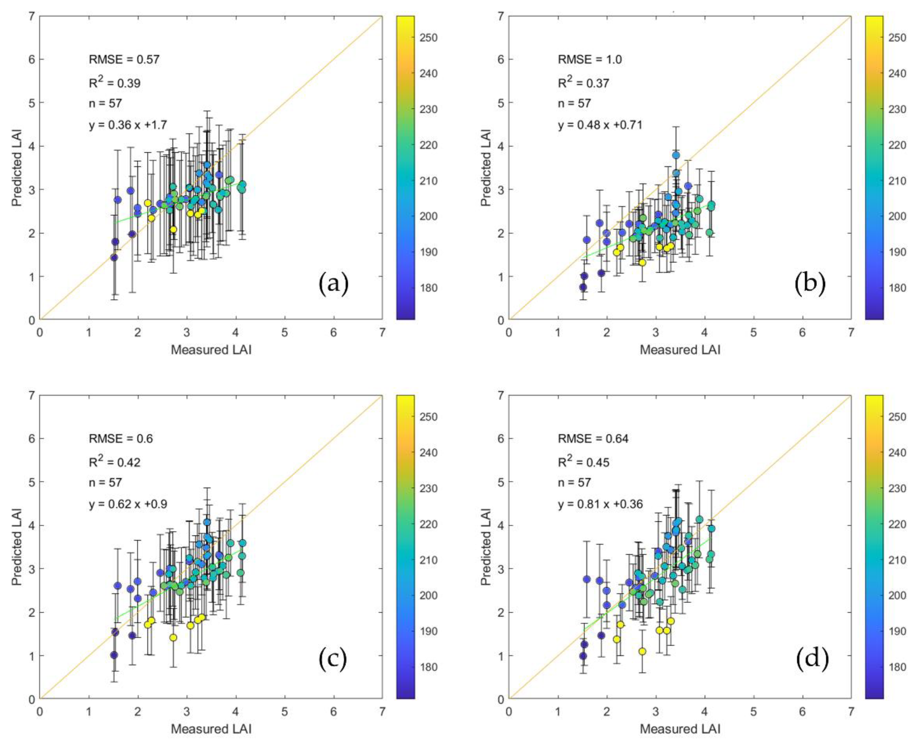
3.3. Accuracy of LAI Inversion at Different Growth Stages

Based on the above comparison of LAI estimations using different inversion strategies, comparable results were obtained for either Landsat 7/8 or Sentinel-2 data. In the following analysis, CIgreen for Landsat 7/8 and a combination of the three Red-edge bands for Sentinel-2 were used as the optimum inversion strategies for their lower RMSE. It was observed that LAI retrieved from the three red-edge bands of Sentinel-2 (Figure 9d) was more accurate (RMSE = 0.64) than LAI derived from CIgreen of Landsat (RMSE = 0.72) during the entire growth season (Figure 8c). In particular, LAI derived from Sentinel-2 performed better around the 1:1 line at high LAI (>3) regions. Similar underestimation was observed at the later growth stages. To further compare the accuracy between Landsat-derived LAI and Sentinel-2-derived LAI, the estimated LAI and measured LAI during the vegetative stage (before DOY 212) was compared. Figure 11a shows that the accuracy of LAI derived from Sentinel-2 improved as RMSE decreased from 0.64 to 0.45 when observation at the reproductive stage was removed (n decreased from 57 to 33) and R2 also increased from 0.45 to 0.68. Figure 11b shows that the accuracy of LAI derived from Landsat improved as RMSE decreased from 0.72 to 0.59 when only LAI estimation at the vegetative stage was validated (n decreased from 47 to 34) and R2 also increased from 0.75 to 0.82. The result indicates that Sentinel-2 still performed better than Landsat at the vegetative stage. Overall, LAI derived from different satellite sensors with high accuracy can be obtained. A combination of multiple RS data can improve the temporal resolution of LAI estimation during the whole growing season.
It is widely acknowledged that crop phenology has great influence on canopy reflectance. To illustrate this further, the accuracies of combined LAI retrievals from three sensors between the vegetative stage (before DOY 212) and the reproductive stage (after DOY 212) were compared. At the vegetative stage, the validation achieved an R2 of 0.74 with a lower RMSE of 0.53 (Figure 12a), which showed much higher accuracy than that at the reproductive stage (0.89 LAI in terms of RMSE and R2 = 0.41 (Figure 12b).

4. Discussion

4.1. Potential and Limitations of LAINet

Compared to the mainstream hand-held LAI measurement instruments (e.g., LAI-2200C), LAINet has an advantage in acquiring time-series field LAI automatically. Compared with other existing automated measurement methods using photos and TLS [11,12,13,14,15,16], the file size of WSN-based LAINet is less bandwidth-intensive, hence, post-processing is less computationally demanding. In principle, both LAINet and PASTIS-57 are based on radiation transmittance to measure PAI, without distinguishing leaves with different chlorophyll contents and from other plant tissues [9,11]. Calibration among all sensors deployed above and below the canopy is a must. For photography-based methods [13,14,15], the calculation of gap fraction from image classification can be a source of uncertainty. These measurement techniques are all vulnerable to adverse weather conditions. The same as in the developing and emerging methods including the LAINet system, there is still a long way to go before operational deployment.
The systematic errors of LAINet measurements should be reduced first. Firstly, elimination of or reduction in the influence by the light environment should be considered. For example, radiation calibration using an integrating sphere ensures consistent quantification of radiation above and below canopy. Multi-day aggregation on daily LAINet measurement is another approach to reduce the influence of daily variation in light environment. Secondly, apparent outliers should be removed to avoid error propagation. For instance, the unrealistic LAI after DOY 212 in 2018 were removed in this study. In addition, an adjustment on LAINet data was done in this study based on field LAI data. A scale of 1.3 was used to adjust LAINet data for improved consistency with LAI-2200C. This was based on an observation by Qu et al. [10] that LAINet seems to be closer to LAIt than LAI-2000 for corn during the 2012 ground experiment in the same study area. Possibly leaf angle distribution (LAD) adopted in the LAINet algorithm may not reflect the true condition of the corn canopy. Deeper analysis on the algorithm may help reveal the issue. However, this is out of the scope of this study. To further investigate this phenomenon, future efforts are needed to explore its authenticity or physical reasons.

4.2. Impact of Inversion Strategies on LAI Estimations

Based on the above comparison of LAI estimations using different inversion strategies in Section 3.2, comparable results were obtained for either Landsat 7/8 or Sentinel-2 among all cases tested. This indicates that the PROSAIL RTM inversion with LUT-based methods is suitable for tracking LAI evolutions with good accuracy. However, the LAI values retrieved using different inversion strategies are slightly different for different satellite data. Overall, the LAIs using CIgreen for Landsat 7/8 and the combination of three Red-edge bands for Sentinel-2 were analyzed ultimately as the optimum inversion strategy for their lower RMSE. LAI derived from Sentinel-2 with an RMSE of 0.64 was more accurate than that derived from Landsat (RMSE = 0.72).
In addition to LAI, other leaf or canopy parameters such as leaf angle distribution and leaf chlorophyll content, also have a substantial contribution to the variability of visible and NIR reflectance. In comparison with the use of band reflectance, the accuracy of LAI retrieval was generally improved when VIs were used. In particular, CIgreen performed the best at estimating LAI with the lowest RMSE (see Figure 8c and Figure 10a). VI was designed to improve the sensitivity to canopy variables (such as LAI), at the same time as suppressing the influence of other influential factors, e.g., impacts from soil reflectance and leaf chlorophyll absorption. From previous studies, CIgreen and EVI2 show a stronger capability to overcome the saturation issues at a high LAI and minimize background influence [48,49]. Spectral reflectance from satellite sensors will be affected by variation of interference factors in the signal path [50]. Hence, the combination of several bands can improve the performance of LAI inversion by weakening these effects partially. Anthony et al. monitored GLAI using the green and red-edge bands [51]. A good performance of the combination of three red-edge bands shown in Figure 9d was found, which was consistent with work demonstrating the value of the red-edge spectral bands in Sentinel-2. EVI2 shows a better performance than NDVI because it is less prone to saturation [50]. In terms of uncertainty, the chlorophyll indices (including CIgreen, and CIred-edge) are sensitive across the entire range of LAI [52] and yielded the lowest RMSE compared with the optical VIs including NDVI and EVI2.

4.3. Difference between LAI Measurement and RS Inversion

The decline in leaf chlorophyll content at the reproductive stage and spectral saturation are potential factors inducing the substantial differences between LAI inversion and field measurement.
Firstly, the variability of leaf chlorophyll content at the vegetative stage is higher than that at the reproductive stage when the proportion of non-photosynthetic components is large. Some research shows that a positive relationship between corn canopy chlorophyll and green LAI goes from linear to non-linear due to the decline in leaf chlorophyll content at the reproductive stage [53]. As satellite remote-sensing is more sensitive to plant photosynthetic components, LAI estimation tends to decrease quickly at the reproductive stage. However, LAINet is sensitive not only to photosynthetic components, but also to non-photosynthetic components to a certain extent. In this respect, the discrepancy between the measured and the estimated LAI can be attributed to the difference in the physical meaning of LAI, namely PAI vs. green LAI.
In addition, when LAI is large, LAI retrievals may underestimate measured LAI due to saturation of spectrum. This phenomenon is more obvious for Landsat-derived LAI (Figure 8c) when CIgreen was used for the inversion.

5. Conclusions

We assessed cornfield LAI estimates derived from Sentinel-2/MSI, Landsat 8/OLI, and Landsat-7/ETM+ through comparison with continuous field LAI measurements collected by LAINet. Based on the results of this experiment, the following conclusions can be made:
(1) The PROSAIL RTM inversion with LUT-based methods is suitable for tracking LAI evolutions with good accuracy. However, the performances of different inversion strategies vary among different satellite data. In this study, CIgreen was optimal to derive Landsat LAI, while a combination of three red-edge bands was optimal to derive Sentinel-2 LAI;
(2) The accuracies of LAI retrievals vary at different phenological growing stages. From the vegetative stage to the reproductive stage, R2 decreased from 0.74 to 0.41 and RMSE increased from 0.53 to 0.89. The decline in leaf chlorophyll content at the reproductive stage and saturation of spectrum are potential factors inducing the differences between LAI inversion and field measurement;
(3) LAINet, a continuous LAI measurement system based on a wireless sensor network technology, has the potential to validate time-series LAI at very low cost. However, more intensive field LAI measurements at different phenological stages and for different crop types will be acquired in future work to diagnose whether LAI measured using LAINet is closer to LAIt or not;
Overall, this study suggests that time-series LAI can be retrieved from multi-source satellite data through model inversion. Our findings will contribute to enhancing the confidence in validating coarse long-term LAI products with time-series measurements by LAINet and multi-source RS data. In the near future, continuous field campaigns using LAINet will be carried out to collect LAI measurements of different crop types.

Author Contributions

Y.Q. provided self-designed LAINet and finalized the scheme design of the field experiments. L.Y., Z.G., Z.W., L.T., and D.W. participated in the LAI field campaigns. T.C. and R.J. also made great contribution in LAI collection using LI-3000 and LAI-2200C. L.Y. conducted data processing, analysis, and original manuscript drafting. J.L., Y.Q., J.S., and Z.C. validated the methods and results. All coauthors have contribution in revising the manuscript. All authors have read and agreed to the published version of the manuscript.

Acknowledgments

We are grateful to the China Scholarship Council (CSC) for providing a scholarship for Yu Lihong to pursue studies at Agriculture and Agri-Food Canada as a joint Ph.D. student.

Funding

This research was supported by the National Natural Science Foundation of China (Grant No. 41671333 and 41531174).

Conflicts of Interest

The authors declare no conflict of interest.

References

  1. Chen, J.M.; Black, T.A. Defining leaf area index for non-flat leaves. Plant Cell Environ. 1992, 15, 421–429. [Google Scholar] [CrossRef]
  2. Chen, J.M.; Pavlic, G.; Brown, L.; Cihlar, J.; Leblanc, S.; White, H.P.; Hall, R.; Peddle, D.; King, D.; Trofymow, J.; et al. Derivation and validation of Canada-wide coarse-resolution leaf area index maps using high-resolution satellite imagery and ground measurements. Remote Sens. Environ. 2002, 80, 165–184. [Google Scholar] [CrossRef]
  3. Myneni, R.B.; Hoffman, S.; Knyazikhin, Y.; Privette, J.L.; Glassy, J.; Tian, Y.; Wang, Y.; Song, X.; Zhang, Y.; Smith, G.R.; et al. Global products of vegetation leaf area and fraction absorbed PAR from year one of MODIS data. Remote Sens. Environ. 2002, 83, 214–231. [Google Scholar] [CrossRef] [Green Version]
  4. GCOS. The Global Observing System for Climate: Implementation Needs (GCOS-200); WMOP: Geneva, Switzerland, 2016. [Google Scholar]
  5. Dong, T.; Liu, J.; Qian, B.; He, L.; Liu, J.; Wang, R.; Jing, Q.; Champagne, C.; McNairn, H.; Powers, J.; et al. Estimating crop biomass using leaf area index derived from Landsat 8 and Sentinel-2 data. ISPRS J. Photogramm. Remote Sens. 2020, 168, 236–250. [Google Scholar] [CrossRef]
  6. Xie, X.; Li, A.; Jin, H.; Tan, J.; Wang, C.; Lei, G.; Zhang, Z.; Bian, J.; Nan, X. Assessment of five satellite-derived LAI datasets for GPP estimations through ecosystem models. Sci. Total. Environ. 2019, 690, 1120–1130. [Google Scholar] [CrossRef]
  7. Waldner, F.; Horan, H.; Chen, Y.; Hochman, Z. High temporal resolution of leaf area data improves empirical estimation of grain yield. Sci. Rep. 2019, 9, 15714. [Google Scholar] [CrossRef] [Green Version]
  8. Yan, G.; Hu, R.; Luo, J.; Weiss, M.; Jiang, H.; Mu, X.; Xie, D.; Zhang, W. Review of indirect optical measurements of leaf area index: Recent advances, challenges, and perspectives. Agric. For. Meteorol. 2019, 265, 390–411. [Google Scholar] [CrossRef]
  9. Qu, Y.; Han, W.; Fu, L.; Li, C.; Song, J.; Zhou, H.; Bo, Y.; Wang, J. LAINet—A wireless sensor network for coniferous forest leaf area index measurement: Design, algorithm and validation. Comput. Electron. Agric. 2014, 108, 200–208. [Google Scholar] [CrossRef]
  10. Qu, Y. Leaf Area Index: Advances in Ground-Based Measurement. In River Basin Management; Springer Science and Business Media LLC: Berlin/Heidelberg, Germany, 2019; pp. 359–378. [Google Scholar]
  11. Brede, B.; Gastellu-Etchegorry, J.-P.; Lauret, N.; Baret, F.; Clevers, J.G.P.W.; Verbesselt, J.; Herold, M. Monitoring Forest Phenology and Leaf Area Index with the Autonomous, Low-Cost Transmittance Sensor PASTiS-57. Remote Sens. 2018, 10, 1032. [Google Scholar] [CrossRef] [Green Version]
  12. Fang, H.; Ye, Y.; Liu, W.; Wei, S.; Ma, L. Continuous estimation of canopy leaf area index (LAI) and clumping index over broadleaf crop fields: An investigation of the PASTIS-57 instrument and smartphone applications. Agric. For. Meteorol. 2018, 2018, 48–61. [Google Scholar] [CrossRef]
  13. Brown, L.A.; Ogutu, B.O.; Dash, J. Tracking forest biophysical properties with automated digital repeat photography: A fisheye perspective using digital hemispherical photography from below the canopy. Agric. For. Meteorol. 2020, 287, 107944. [Google Scholar] [CrossRef]
  14. Toda, M.; Richardson, A.D. Estimation of plant area index and phenological transition dates from digital repeat photography and radiometric approaches in a hardwood forest in the Northeastern United States. Agric. For. Meteorol. 2018, 249, 457–466. [Google Scholar] [CrossRef]
  15. Ryu, Y.; Verfaillie, J.; Macfarlane, C.; Kobayashi, H.; Sonnentag, O.; Vargas, R.; Ma, S.; Baldocchi, D. Continuous observation of tree leaf area index at ecosystem scale using upward-pointing digital cameras. Remote Sens. Environ. 2012, 126, 116–125. [Google Scholar] [CrossRef]
  16. Culvenor, D.S.; Newnham, G.J.; Mellor, A.; Sims, N.C.; Haywood, A. Automated In-Situ Laser Scanner for Monitoring Forest Leaf Area Index. Sensors 2014, 14, 14994–15008. [Google Scholar] [CrossRef] [PubMed] [Green Version]
  17. Atzberger, C.; Darvishzadeh, R.; Schlerf, M.; Le Maire, G. Suitability and adaptation of PROSAIL radiative transfer model for hyperspectral grassland studies. Remote Sens. Lett. 2013, 4, 55–64. [Google Scholar] [CrossRef]
  18. Jacquemoud, S.; Baret, F. PROSPECT: A model of leaf optical properties spectra. Remote Sens. Environ. 1990, 34, 75–91. [Google Scholar] [CrossRef]
  19. Verhoef, W. Light scattering by leaf layers with application to canopy reflectance modeling: The SAIL model. Remote Sens. Environ. 1984, 16, 125–141. [Google Scholar] [CrossRef] [Green Version]
  20. Banskota, A.; Serbin, S.P.; Wynne, R.H.; Thomas, V.A.; Falkowski, M.J.; Kayastha, N.; Gastellu-Etchegorry, J.-P.; Townsend, P.A. An LUT-Based Inversion of DART Model to Estimate Forest LAI from Hyperspectral Data. IEEE J. Sel. Top. Appl. Earth Obs. Remote Sens. 2015, 8, 3147–3160. [Google Scholar] [CrossRef]
  21. Campos-Taberner, M.; García-Haro, F.J.; Camps-Valls, G.; Grau-Muedra, G.; Nutini, F.; Crema, A.; Boschetti, M. Multitemporal and multiresolution leaf area index retrieval for operational local rice crop monitoring. Remote Sens. Environ. 2016, 187, 102–118. [Google Scholar] [CrossRef]
  22. Jin, H.; Xu, W.; Li, A.; Xie, X.; Zhang, Z.; Xia, H. Spatially and Temporally Continuous Leaf Area Index Mapping for Crops through Assimilation of Multi-resolution Satellite Data. Remote Sens. 2019, 11, 2517. [Google Scholar] [CrossRef] [Green Version]
  23. Fang, H.; Baret, F.; Plummer, S.; Schaepman-Strub, G. An Overview of Global Leaf Area Index (LAI): Methods, Products, Validation, and Applications. Rev. Geophys. 2019, 57, 739–799. [Google Scholar] [CrossRef]
  24. Yang, W.; Tan, B.; Huang, D.; Rautiainen, M.; Shabanov, N.V.; Wang, Y.; Privette, J.L.; Huemmrich, K.; Fensholt, R.; Sandholt, I.; et al. MODIS leaf area index products: From validation to algorithm improvement. IEEE Trans. Geosci. Remote Sens. 2006, 44, 1885–1898. [Google Scholar] [CrossRef]
  25. Liang, S.; Fang, H.; Chen, M.; Shuey, C.J.; Walthall, C.; Daughtry, C.S.T.; Morisette, J.; Schaaf, C.B.; Strahler, A. Validating MODIS land surface reflectance and albedo products: Methods and preliminary results. Remote Sens. Environ. 2002, 83, 149–162. [Google Scholar] [CrossRef]
  26. Morisette, J.; Baret, F.; Privette, J.; Myneni, R.; Nickeson, J.; Garrigues, S.; Shabanov, N.; Weiss, M.; Fernandes, R.; Leblanc, S.; et al. Validation of global moderate-resolution LAI products: A framework proposed within the CEOS land product validation subgroup. IEEE Trans. Geosci. Remote Sens. 2006, 44, 1804–1817. [Google Scholar] [CrossRef] [Green Version]
  27. Fang, H.; Zhang, Y.; Wei, S.; Li, W.; Ye, Y.; Sun, T.; Liu, W. Validation of global moderate resolution leaf area index (LAI) products over croplands in northeastern China. Remote Sens. Environ. 2019, 233, 111377. [Google Scholar] [CrossRef]
  28. Yan, K.; Park, T.; Chen, C.; Xu, B.; Song, W.; Yang, B.; Zeng, Y.; Liu, Z.; Yan, G.; Knyazikhin, Y.; et al. Generating Global Products of LAI and FPAR from SNPP-VIIRS Data: Theoretical Background and Implementation. IEEE Trans. Geosci. Remote Sens. 2018, 56, 2119–2137. [Google Scholar] [CrossRef]
  29. Xiao, Z.; Liang, S.; Wang, J.; Xiang, Y.; Zhao, X.; Song, J. Long-Time-Series Global Land Surface Satellite Leaf Area Index Product Derived from MODIS and AVHRR Surface Reflectance. IEEE Trans. Geosci. Remote Sens. 2016, 54, 5301–5318. [Google Scholar] [CrossRef]
  30. Verger, A.; Baret, F.; Weiss, M. GEOV2/VGT: Near real time estimation of global biophysical variables from VEGETATION-P data. In Proceedings of the MultiTemp 2013: 7th International Workshop on the Analysis of Multi-temporal Remote Sensing Images, Banff, AB, Canada, 25–27 June 2013; pp. 1–4. [Google Scholar]
  31. Kimm, H.; Guan, K.; Jiang, C.; Peng, B.; Gentry, L.F.; Wilkin, S.C.; Wang, S.; Cai, Y.; Bernacchi, C.J.; Peng, J.; et al. Deriving high-spatiotemporal-resolution leaf area index for agroecosystems in the U.S. Corn Belt using Planet Labs CubeSat and STAIR fusion data. Remote Sens. Environ. 2020, 239, 111615. [Google Scholar] [CrossRef]
  32. Beck, H.E.; Zimmermann, N.E.; McVicar, T.R.; Vergopolan, N.; Berg, A.; Wood, E.F. Present and future Köppen-Geiger climate classification maps at 1-km resolution. Sci. Data 2018, 5, 180214. [Google Scholar] [CrossRef] [Green Version]
  33. Peel, M.C.; Finlayson, B.L.; McMahon, T.A. Updated world map of the Köppen-Geiger climate classification. Hydrol. Earth Syst. Sci. 2007, 11, 1633–1644. [Google Scholar] [CrossRef] [Green Version]
  34. Yan, K.; Park, T.; Yan, G.; Liu, Z.; Yang, B.; Chen, C.; Nemani, R.; Knyazikhin, Y.; Myneni, R.B. Evaluation of MODIS LAI/FPAR Product Collection 6. Part 2: Validation and Intercomparison. Remote Sens. 2016, 8, 460. [Google Scholar] [CrossRef] [Green Version]
  35. Dong, T.; Liu, J.; Shang, J.; Qian, B.; Ma, B.; Kovacs, J.M.; Walters, D.; Jiao, X.; Geng, X.; Shi, Y. Assessment of red-edge vegetation indices for crop leaf area index estimation. Remote Sens. Environ. 2019, 222, 133–143. [Google Scholar] [CrossRef]
  36. Main-Knorn, M.; Pflug, B.; Louis, J.; Debaecker, V.; Müller-Wilms, U.; Gascon, F. Sen2Cor for Sentinel-2. In Proceedings of the Image and Signal Processing for Remote Sensing XXIII, Warsaw, Poland, 11–13 September 2017; SPIE: Bellingham, WA, USA, 2017; p. 1042704. [Google Scholar]
  37. Lang, A. Simplified estimate of leaf area index from transmittance of the sun’s beam. Agric. For. Meteorol. 1987, 41, 179–186. [Google Scholar] [CrossRef]
  38. Qu, Y.; Zhu, Y.; Han, W.; Wang, J.; Ma, M. Crop Leaf Area Index Observations with a Wireless Sensor Network and Its Potential for Validating Remote Sensing Products. IEEE J. Sel. Top. Appl. Earth Obs. Remote Sens. 2014, 7, 431–444. [Google Scholar] [CrossRef]
  39. Fu, G.; Wu, J.-S. Validation of MODIS collection 6 FPAR/LAI in the alpine grassland of the Northern Tibetan Plateau. Remote Sens. Lett. 2017, 8, 831–838. [Google Scholar] [CrossRef]
  40. Wang, T.; Qu, Y.; Xia, Z.; Ma, T.; Liu, Z. Multi-Scale Validation of MODIS LAI Products Based on Crop Growth Period. ISPRS Int. J. Geo-Inf. 2019, 8, 547. [Google Scholar] [CrossRef] [Green Version]
  41. Qu, Y.; Han, W.; Ma, M. Retrieval of a Temporal High-Resolution Leaf Area Index (LAI) by Combining MODIS LAI and ASTER Reflectance Data. Remote Sens. 2014, 7, 195–210. [Google Scholar] [CrossRef]
  42. Rouse, J.; Haas, R.; Schell, J.; Deering, D.W. Monitoring Vegetation Systems in the Great Plains with ERTS; NASA: Washington, DC, USA, 1974; Volume 351, p. 309.
  43. Jiang, Z.; Huete, A.; Didan, K.; Miura, T. Development of a two-band enhanced vegetation index without a blue band. Remote Sens. Environ. 2008, 112, 3833–3845. [Google Scholar] [CrossRef]
  44. Gitelson, A.A.; Gritz, Y.; Merzlyak, M.N. Relationships between leaf chlorophyll content and spectral reflectance and algorithms for non-destructive chlorophyll assessment in higher plant leaves. J. Plant Physiol. 2003, 160, 271–282. [Google Scholar] [CrossRef]
  45. Li, H.; Liu, G.; Liu, Q.; Chen, Z.; Huang, C. Retrieval of Winter Wheat Leaf Area Index from Chinese GF-1 Satellite Data Using the PROSAIL Model. Sensors 2018, 18, 1120. [Google Scholar] [CrossRef] [Green Version]
  46. Richter, K.; Hank, T.B.; Vuolo, F.; Mauser, W.; D’Urso, G. Optimal Exploitation of the Sentinel-2 Spectral Capabilities for Crop Leaf Area Index Mapping. Remote Sens. 2012, 4, 561–582. [Google Scholar] [CrossRef] [Green Version]
  47. Verger, A.; Baret, F.; Camacho, F. Optimal modalities for radiative transfer-neural network estimation of canopy biophysical characteristics: Evaluation over an agricultural area with CHRIS/PROBA observations. Remote Sens. Environ. 2011, 115, 415–426. [Google Scholar] [CrossRef]
  48. Gitelson, A.A.; Viña, A.; Ciganda, V.; Rundquist, D.C.; Arkebauer, T.J. Remote estimation of canopy chlorophyll content in crops. Geophys. Res. Lett. 2005, 32, 32. [Google Scholar] [CrossRef] [Green Version]
  49. Zou, X.; Mõttus, M. Sensitivity of Common Vegetation Indices to the Canopy Structure of Field Crops. Remote Sens. 2017, 9, 994. [Google Scholar] [CrossRef] [Green Version]
  50. Liu, J.; Pattey, E.; Jégo, G. Assessment of vegetation indices for regional crop green LAI estimation from Landsat images over multiple growing seasons. Remote Sens. Environ. 2012, 123, 347–358. [Google Scholar] [CrossRef]
  51. Nguy-Robertson, A.; Peng, Y.; Gitelson, A.A.; Arkebauer, T.J.; Pimstein, A.; Herrmann, I.; Karnieli, A.; Rundquist, D.C.; Bonfil, D.J. Estimating green LAI in four crops: Potential of determining optimal spectral bands for a universal algorithm. Agric. For. Meteorol. 2014, 192, 140–148. [Google Scholar] [CrossRef]
  52. Viña, A.; Gitelson, A.A.; Nguy-Robertson, A.; Peng, Y. Comparison of different vegetation indices for the remote assessment of green leaf area index of crops. Remote Sens. Environ. 2011, 115, 3468–3478. [Google Scholar] [CrossRef]
  53. Gitelson, A.A.; Peng, Y.; Arkebauer, T.J.; Schepers, J. Relationships between gross primary production, green LAI, and canopy chlorophyll content in maize: Implications for remote sensing of primary production. Remote Sens. Environ. 2014, 144, 65–72. [Google Scholar] [CrossRef]
Figure 1. The study area (left) and field observation plots in 2018 and 2019 (right). The background map was a color composite Sentinel-2B image (Band 4-3-2) acquired on 30th July 2019.
Remotesensing 12 03304 g001
Figure 2. Temporal distribution of in situ leaf area index (LAI) measurement using three instruments during the 2018 and 2019 seasons. DOY stands for day of year (for instance, DOY 210 is the 210th day of this year).
Remotesensing 12 03304 g002
Figure 3. Process flow of model derivation and validation
Remotesensing 12 03304 g003
Figure 4. Temporal variation in field LAI measurements collected by LAINet, LAI-2200C, and LI-3000 at 3 corn plots in 2018. DOY stands for day of year.
Remotesensing 12 03304 g004
Figure 5. Temporal variation in field LAI measurements collected by LAINet, LAI-2200C, and LI-3000 at 6 corn plots in 2019. DOY stands for day of year.
Remotesensing 12 03304 g005
Figure 6. Relationship between field LAI measurements and EVI2 for 2018 (a) and 2019 (b). The color bar indicates observation dates (i.e., DOY, day of year).
Remotesensing 12 03304 g006
Figure 7. Comparison of estimated and measured LAI using reflectance-based look-up-table (LUT) for Landsat 7/8. The spectral bands used for inversion correspond to (a) R; (b) R and NIR; (c) R, NIR, SWIR1 and SWIR2; (d) SWIR1 and SWIR2. Error bar represents the standard deviation of LAI retrievals. Color bar represents DOY (i.e., day of year) of images.
Remotesensing 12 03304 g007
Figure 8. Comparison of estimated and measured LAI using VI-based LUT for Landsat 7/8. The VIs used for inversion correspond to (a) NDVI; (b) EVI2; (c) CIgreen. Error bar represents the standard deviation of LAI retrievals. Color bar represents DOY (i.e., day of year) of images.
Remotesensing 12 03304 g008
Figure 9. Comparison of LAI measured in situ and that estimated from reflectance-based LUT from Sentinel-2 data. The spectral bands used for inversion correspond to (a) G; (b) R, and NIR; (c) red-edge 1 and NIR; (d) red-edge 1, red-edge 2 and red-edge 3. Error bar represents the standard deviation of LAI retrievals. Color bar represents DOY (i.e., day of year) of images.
Remotesensing 12 03304 g009
Figure 10. Comparison of LAI measured in situ and that estimated from VI-based LUT from Sentinel-2 data. The VIs used for inversion correspond to (a) CIgreen; (b) CIred-edge1; (c) NDVI; (d) EVI2. Error bar represents the standard deviation of LAI retrievals. Color bar represents DOY (i.e., day of year) of images.
Remotesensing 12 03304 g010
Figure 11. Comparison between measured and estimated LAI (a) derived from Sentinel-2, (b) Landsat 7/8 before DOY (i.e., day of year) 212. (The 1:1 line is shown in red)
Remotesensing 12 03304 g011
Figure 12. Comparison between measured and estimated LAI (a) before and (b) after DOY (i.e., day of year) 212.
Remotesensing 12 03304 g012
Table 1. Acquisition dates of remote-sensing (RS) data collected over the study area for 2018 and 2019. DOY stands for day of year.
YearsSensorsDOY
2018Sentinel-2 MSI171, 196, 201, 206, 211, 216, 221, 226, 256
Landsat 8 OLI168, 200, 216, 232
Landsat 7 ETM+192, 256
2019Sentinel-2 MSI181, 186, 211, 216, 226, 256
Landsat 8 OLI203
Landsat 7 ETM+163, 179, 195, 211, 227, 243
Table 2. List of canopy and leaf parameters applied in PROSAIL radiative transfer modelling (RTM) for modeling canopy surface reflectance.
ParametersUnitsValue/Range
N –leaf structural parameter 1–2.5
C a b –leaf chlorophyll content μ g / cm 2 5–90
C w –equivalent water thickness cm 0.004–0.07
C m –leaf dry matter content g / cm 2 0.0026–0.0132
Brown–brown pigment content 0
Car–carotenoid content μ g / cm 2 0.6–15.91
LAI–leaf area index m 2 / m 2 0–7.0
ALA–average leaf angle degree 20–80
s k y l –diffuse/total radiation 0.1
ρ s o i l –soil brightness coefficient 0–1
H s p o t –hot spot effect 0.05–0.1
S Z A –solar zenith angle degree acquired from metadata
V Z A –view zenith angle degree acquired from metadata
psi –relative azimuth angle degree 0
Table 3. Vegetation indices used in this study.
Vegetation IndexFormulasSensorReferences
Normalized Difference Vegetation Index NDVI=(NIR−R)/(NIR+R)Landsat/Sentinel-2[42]
Enhanced Vegetation Index 2EVI2=2.5(NIR−R)/(NIR+2.4R+1)Landsat/Sentinel-2[43]
Green Chlorophyll index CIgreen=NIR/G-1Landsat/Sentinel-2[44]
Red-edge Chlorophyll index CIred-edge=NIR/Red-edge 1Sentinel-2[44]
Table 4. Statistics of three kinds of field LAI measurements in 2019.
PlotLAINetLAI-2200CLI-3000RPE/LAINetRPE/LAI-2200C
Plot33.713.663.642.18%0.76%
Plot55.043.204.707.13%−31.88%
Plot63.292.544.23−22.36%−40.01%
Mean4.013.144.19−4.35%−23.71%

