Article

Ensemble Learning Approaches Based on Covariance Pooling of CNN Features for High Resolution Remote Sensing Scene Classification

1
CNRS, IMS, UMR n∘5218, Groupe Signal et Image, University of Bordeaux, F-33405 Talence, France
2
RIKEN Center for Advanced Intelligence Project (AIP), RIKEN, Tokyo 103-0027, Japan
*
Author to whom correspondence should be addressed.
Remote Sens. 2020, 12(20), 3292; https://doi.org/10.3390/rs12203292
Submission received: 31 August 2020 / Revised: 23 September 2020 / Accepted: 2 October 2020 / Published: 10 October 2020
(This article belongs to the Special Issue Feature-Based Methods for Remote Sensing Image Classification)

Abstract

:
Remote sensing image scene classification, which consists of labeling remote sensing images with a set of categories based on their content, has received remarkable attention for many applications such as land use mapping. Standard approaches are based on the multi-layer representation of first-order convolutional neural network (CNN) features. However, second-order CNNs have recently been shown to outperform traditional first-order CNNs for many computer vision tasks. Hence, the aim of this paper is to show the use of second-order statistics of CNN features for remote sensing scene classification. This takes the form of covariance matrices computed locally or globally on the output of a CNN. However, these datapoints do not lie in an Euclidean space but a Riemannian manifold. To manipulate them, Euclidean tools are not adapted. Other metrics should be considered such as the log-Euclidean one. This consists of projecting the set of covariance matrices on a tangent space defined at a reference point. In this tangent plane, which is a vector space, conventional machine learning algorithms can be considered, such as the Fisher vector encoding or SVM classifier. Based on this log-Euclidean framework, we propose a novel transfer learning approach composed of two hybrid architectures based on covariance pooling of CNN features, the first is local and the second is global. They rely on the extraction of features from models pre-trained on the ImageNet dataset processed with some machine learning algorithms. The first hybrid architecture consists of an ensemble learning approach with the log-Euclidean Fisher vector encoding of region covariance matrices computed locally on the first layers of a CNN. The second one concerns an ensemble learning approach based on the covariance pooling of CNN features extracted globally from the deepest layers. These two ensemble learning approaches are then combined together based on the strategy of the most diverse ensembles. For validation and comparison purposes, the proposed approach is tested on various challenging remote sensing datasets. Experimental results exhibit a significant gain of approximately 2 % in overall accuracy for the proposed approach compared to a similar state-of-the-art method based on covariance pooling of CNN features (on the UC Merced dataset).

Graphical Abstract

1. Introduction

The aim of a supervised classification algorithm consists of labeling an image with the corresponding class according to its content. Conventional approaches are based on encoding handcrafted features with, for example, the bag of words model (BoW) [1], the vector of locally aggregated descriptors (VLAD) [2,3] or the Fisher vectors (FV) [4,5,6]. These latter strategies have proved successful results in a wide range of applications such as image classification [4,7,8], text retrieval [9], action and face recognition [10], etc.
Recently, the emergence of deep learning algorithms has been demonstrated to outperform benchmark machine learning methods in many situations. In fact, neural networks are constructed to model the human brain, where each layer is responsible for automatically extracting and learning specific features from the input images [11]. One of the most popular neural networks is the convolutional neural network (CNN), which has become a standard for image classification problems [12,13]. CNN is built from various hidden layers performing different kinds of transformation, such as convolutions, pooling, and activation functions.
In recent years, in order to benefit from both CNN architectures and encoding methods, many authors have focus on proposing hybrid architectures that consist of combining deep neural network architecture with FV/VLAD descriptors. For example, Perronnin et al., have introduced, in [14] a network of fully connected layers trained on the FV descriptors. Inspired by the multi-layer structure of neural networks, Simonyan et al., proposed, in [15], the Fisher network, which is composed of several stacked FV layers. In the same spirit, the NetVLAD layer has been proposed in [16] to mimick a VLAD layer. To benefit of multi-layer representation, other strategies include the FV or VLAD encoding of CNN features from different layers of the network [17,18,19,20]. Nevertheless, all these strategies do not exploit second-order statistics, i.e., dependencies between features, which have been shown to be important in the human visual recognition process [21].
To this aim, some authors have dedicated their works to exploiting the information behind second-order statistics using covariance matrix features. These have proved to be highly effective in diverse classification tasks, including person re-identification, texture recognition, material categorization or EEG classification in brain–computer interfaces to cite a few of them [10,22,23,24]. Several works have been proposed to extend the encoding formalism to covariance matrix descriptors. Therefore, since covariance matrices are symmetric positive definite (SPD) matrices, conventional Euclidean tools are not adapted. To deal with covariance matrices geometry, two Riemannian metrics are usually considered: the log-Euclidean and the affine-invariant Riemannian metrics. Since then, some authors have proposed to extend the usual coding methods to these two metrics, yielding to the proposition of the following approaches: the log-Euclidean bag of words (LE BoW) [25,26], the bag of Riemannian words (BoRW) [27], the log-Euclidean vector of locally aggregated descriptors (LE VLAD) [10] and the intrinsic Riemannian vector of locally aggregated descriptors (RVLAD) [10]. Recently, FV descriptors extended to SPD matrices have been proposed. This has involved the log-Euclidean Fisher vectors (LE FV) [28] and the Riemannian Fisher vectors (RFV) [29,30,31]. When analyzing those two metrics, log-Euclidean and affine-invariant Riemannian metrics offer several invariance properties and can obtain comparable results for a large variety of applications [31,32] compared to the Euclidean metric. However, the log-Euclidean approach is much more straightforward. To model covariance matrices that lie in a Riemannian manifold, it merely consists in projecting them in a tangent space of a reference point classically chosen equal to the identity matrix.
On the other hand, traditional CNN models capture only first-order statistics. To benefit from both second-order statistics and deep learning architectures, different second-order convolutional neural networks architectures have recently emerged [33,34,35,36,37,38,39,40] for many applications including fine-grained classification. One first attempt was the pooled covariance matrix from CNN outputs [33]. Later, He et al. presented in [35] a multi-layer version: the multi-layer stacked covariance pooling (MSCP). One other way to exploit second-order statistics in a deep neural network is the Riemannian SPD matrix network (SPDNet) [36]. The idea behind this network is to mimick the classical CNN fully connected convolution-like layers and rectified linear units (ReLU)-like layers to data, which do not lie in an Euclidean space. For that, the bilinear mapping (BiMap) layers and eigenvalue rectification (ReEig) layers were proposed. Inspired by this work, Yu et al. have introduced in [37] a second-order CNN (SO-CNN), which is trained in an end-to-end manner. However, for these models, second-order representation is introduced only for the deepest layers. To overcome this issue, Gao et al. [39] have proposed the global second-order pooling (GSoP) convolutional networks which permit to introduce higher-order representation in earlier layers. Nevertheless, training such a deep CNN model from scratch requires a huge labeled training set. Recently, the remote sensing community has started to build large scale datasets that can serve as pre-training, such as the BigEarthNet composed by Sentinel-2 image patches [41]. However, for many practical applications, most of the remote sensing datasets are quite small.
Many authors have proposed several ideas to overcome this issue such as using a new kind of neural network called capsule network [42] which has the ability to work with a small amount of training data. Compared to convolutional neural network, capsule network allows to address the “Picasso problem" in image recognition, i.e., images that show the right components but have not the right spatial relationships. For example, for a face image, the location of the eye and ear are swapped. For our application of remote sensing scene classification, this is not critical. For instance, in an harbour scene, the location of the scene elements (boats, pontoon, …) in the image is not so important. The key point is that the network is able to recognize them. Another effective solution for limited training set consists of transfer learning. In that case, CNN models are considered as feature extractors. Classically, deep CNN models pre-trained on the ImageNet dataset are used. Then, features are extracted from a single or multiple layers and processed with some machine learning algorithms. This technique has been proved to be efficient and permits outperforming traditional handcrafted feature-based methods [13]. In a recent paper, Pires de Lima et al. have shown that transfer learning strategies based on feature extraction are among the best approaches for remote sensing scene classification, especially for the dataset with a low number of training samples [
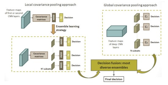
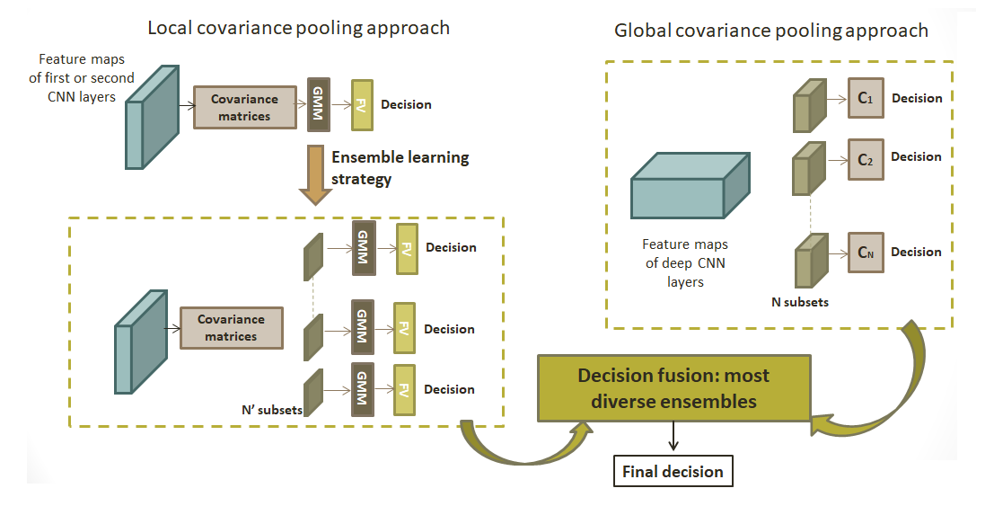
43]. In this context, in order to the benefit of pre-trained deep neural networks and second-order representations, this work aims at proposing a novel ensemble learning approach based on covariance pooling of CNN features for remote sensing scene classification. It consists of a combination of two hybrid architectures exploiting second-order features. The former is based on the log-Euclidean Fisher vector encoding of region covariance matrices computed locally on the first layers of a CNN [28] and its extension to the use of an ensemble learning strategy to combine multiple classifiers. The latter concerns an ensemble learning approach based on the covariance pooling of CNN features extracted from deeper layers [44].
In summary, second-order representation (i.e., covariance pooling) has been shown to be useful for many signal and image processing tasks. Recently, in the remote sensing community, some works have shown interest in these second-order features for various remote sensing applications (e.g., remote sensing scene classification, texture recognition) [35,40,45,46]. Motivated by these works and the success of deep neural networks, we have recently proposed two hybrid transfer learning approaches based on covariance pooling of CNN features [28,44]. These two methods use either local or global second-order representation of CNN features. The main motivation of this journal paper is to unify these works by presenting a transfer learning approach which benefit of these approaches. The main contributions of the paper can be summarized as follows:
  • We propose a transfer learning approach, which efficiently combine local and global second-order representation of CNN features. For the local one, an ensemble learning extension of our log-Euclidean Fisher vector encoding of region covariance matrices [28] is introduced. For the global one, our covariance pooling of deepest CNN features is considered [44].
  • An ensemble learning approach based on the most diverse ensembles is proposed to combine these decisions and enhance the classification performance.
  • This transfer learning is validated on different labeled remote sensing datasets to illustrate its efficiency. Three are publicly available, namely UC Merced Land Use, SIRI-WHU and AID datasets. Two others are internal datasets, oyster racks and maritime pine forest datasets, which are manually labeled by thematic experts.
The paper is structured as follows. Since the second-order representation of CNN features is at the core of the paper, Section 2 gives the mathematical background for the log-Euclidean representation of a covariance matrix. Next, Section 3 introduces the proposed ensemble learning approach based on the log-Euclidean Fisher vector encoding of region covariance matrices. Then, Section 4 recalls our ensemble learning approach based on covariance pooling (ELCP) of CNN features. In order to combine these two methods, Section 5 presents the fusion scheme based on the most diverse ensembles. Next, Section 6 summarizes a series of experiments performed on remote sensing scene classification. And finally, Section 7 provides the main conclusions and perspectives of this work.

2. Log-Euclidean Framework for Second-Order Statistics of CNN Features

In the literature, second-order statistics have been proved to play an important role in the human visual recognition process [21]. In practice, the covariance matrix of handcrafted descriptors, textural or deep convolutional features is computed and integrated into the classification algorithm. Since covariance matrices are symmetric positive definite (SPD) matrices, they have a specific geometry, and standard Euclidean tools are not adapted. The present section aims at explaining the geometry of SPD matrices and classical metrics used to manipulate these data. In fact, these datapoints lie inside the cone of positive definite matrices that is a Riemannian manifold.
Therefore, applying standard Euclidean operations on covariance matrices, for instance, computing the Euclidean distance between two covariance matrices, may lead to undesirable results such as the swelling effect as observed in [47]. Many authors have raised the need of intrinsic tools to analyze SPD matrices [32,48]. As pointed out by Pennec et al., the log-Euclidean and the affine invariant Riemannian metrics enjoy desirable invariance properties compared to the Euclidean metric. The affine invariant Riemannian distance has the property of being invariant by affine transformations.
Even if the log-Euclidean metric does not yield full affine invariance, it is invariant by similarity (orthogonal transformation and scaling). The computations using this metric could be invariant with respect to a change of coordinates obtained by a similarity. From a practical point of view, Arsigny et al., have shown in [32] that affine invariant and log-Euclidean frameworks perform better than the Euclidean one for the interpolation and regularization of their synthetic and clinical 3D diffusion tensor magnetic resonance imaging (DT-MRI) data. This has the advantage of more accurately capturing the underlying scatter of the data points (that are covariance matrices) than is possible with methods that treat data points as elements in a vector space. For many applications, the log-Euclidean framework has shown competitive results compared to the affine invariant Riemannian one [31,
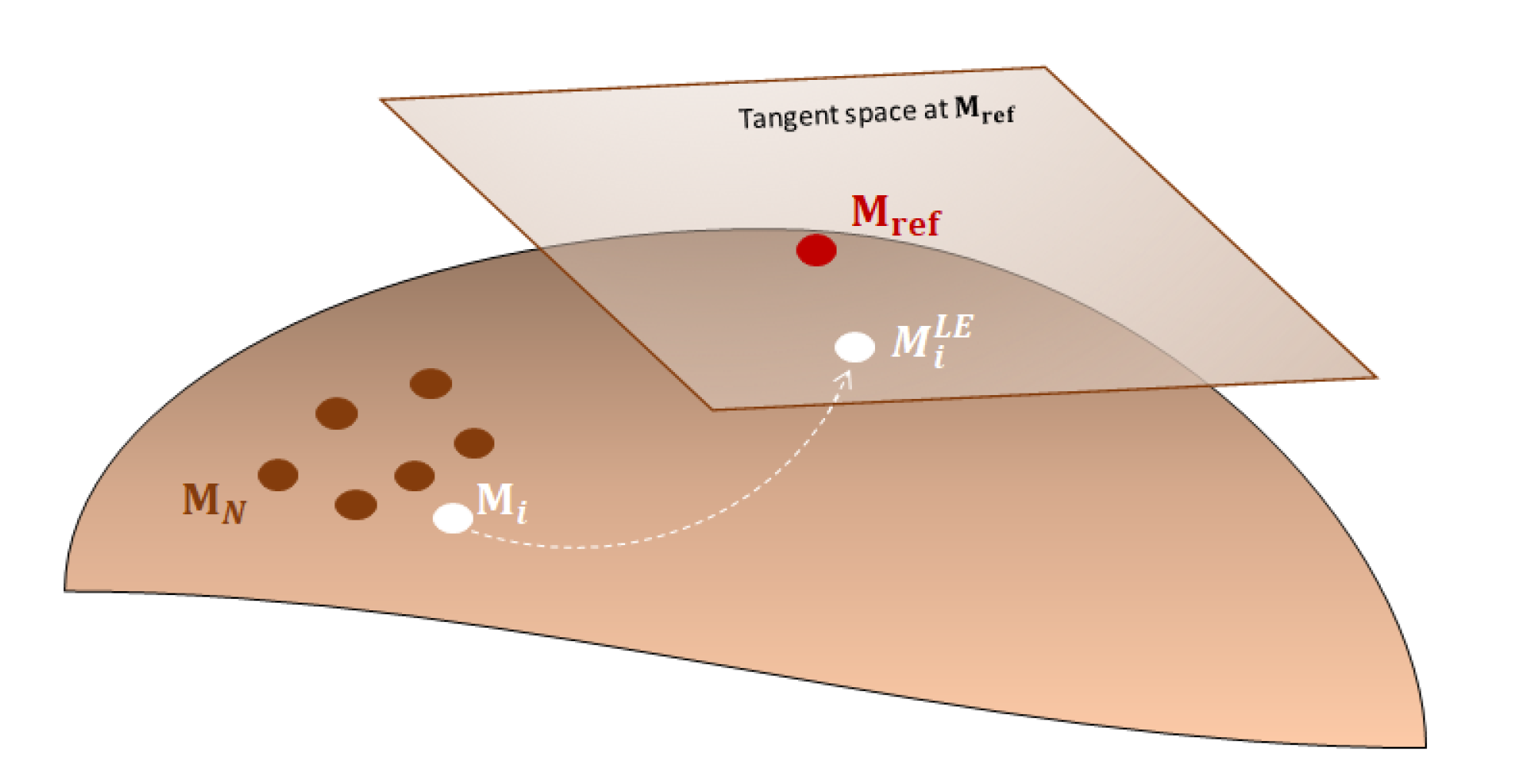
32]. This log-Euclidean framework is considered in this paper for its efficiency and ease of use. The basic principle is the following. Each covariance matrix M n is mapped on the tangent space, as illustrated in Figure 1 that locally flattens the manifold via the tangent space approximation. This consists of projecting covariance matrices onto a common tangent space of this manifold at the reference point M r e f via the log map operator [26,32,45] defined as:
m n T M r e f = Log M r e f M n
= M r e f log M r e f 1 M n .
m n T M r e f means that covariance matrix M n is projected on the tangent space at the reference point M r e f . Then, to get the vector representation, a vectorization operation Vec() is performed such that:
Vec ( X ) = X 11 , 2 X 12 , , 2 X 1 d , X 22 , 2 X 23 , , X d d ,
with X i j the elements of X at row i and column j. Those two operations yield to the definition of the log-Euclidean vector representation of M n computed at the reference point M r e f , denoted m n T M r e f R d ( d + 1 ) 2 where:
m n T M r e f = Vec Log M r e f ( M n ) .
These covariance matrices are projected on the tangent space at M r e f ; they lie in a vector space where conventional image processing and machine learning methods can be used. Within this framework, the tangent space is computed at a reference point M r e f as shown in (1). Different choices can be made for this reference point, such as the identity matrix, the center of mass or the median. The use of the identity matrix I d for this latter is undoubtedly the simplest and the most usual way to map covariance matrices on the tangent space. This choice will be made for the following. In that case, the log map operator in Equation (1) vanishes to:
Log I d ( M n ) = log ( M n ) .
This consists of computing the ordinary matrix logarithm. Let A = V D V T be the eigenvalue decomposition of an SPD matrix, the logarithm is defined as: log ( A ) = V log ( D ) V T . Since D is the diagonal matrix of eigenvalues, log ( D ) is also a diagonal matrix whose diagonal elements are the logarithm of the eigenvalues. In the next two sections, this log-Euclidean framework is employed for two hybrid architectures where the covariance matrix is computed for CNN features.

3. Local Covariance Pooling: Ensemble Log-Euclidean Fisher Vector Architecture

A scene image is composed by a set of visual elements. For example, an harbour scene is formed by many objects such as boat, water, pontoon, … In this context, coding based methods such as FV or VLAD descriptors have reached the state-of-the-art at the beginning of the 2000’s [2,3,4]. These methods relies on the creation of a codebook where codewords represent meaningful object parts of the scene. More recently, deep learning models (and CNN in particular) have shown to outperform these coding methods by a significant margin. For instance, on the ImageNet large scale visual recognition challenge, deep learning based methods have won since 2012 [13]. In order to benefit from both strategies, in the recent literature on scene classification, many authors have introduced hybrid architectures that combine CNN with some coding methods. For example, Perronnin et al. [14] have proposed a network of fully connected layers trained on the FV descriptors. Simonyan et al. introduced in [15] the Fisher network, which is composed of several stacked FV layers. Later, Arandjelovic et al. [16] proposed the NetVLAD layer, which mimicks the VLAD layer. Building on the success of those latter hybrid architectures, more attention is given to a particular approach introduced in [20]. In that paper, Li et al. have proposed a hybrid structure, which consists of encoding each output of the convolutional layers of a pre-trained neural network with FV. This technique has demonstrated competitive results for remote sensing scene classification. To capture various scale phenomenons when applying the FV encoding, a Gaussian pyramid is considered. This permits generating multiscale images by using a Gaussian smoothing and sub-sampling at different scales as detailed in [20]. Classification results have demonstrated the interest of using multiscale images compared to a single input image. Therefore, a pyramid of three scale levels is retained in the following. Those multiscale images are fed into the CNN model, allowing the extraction of convolutional features which are then concatenated before being encoded with FV. Note that CNN models are used only to extract deep features without any retraining from scratch or fine-tuning. In fact, once the multiscale features are extracted from each convolutional layer, an individual codebook is generated. In this approach, the dimension K of the codebook is the same for all the layers. The CNN features are then encoded with the improved FV [
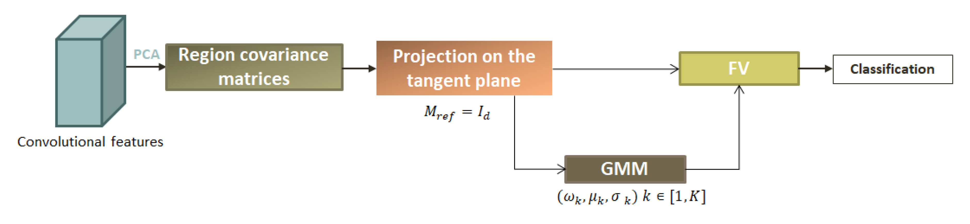
5]. Next, those FVs are fused to represent the mid-level feature vectors of a scene image. Therefore, this approach does not consider second-order features, which have proved to be efficient in many classification problems and have shown to outperform first-order features for many image processing applications, including material recognition and person re-identification. To this aim, we have proposed in [28] a novel hybrid architecture named Hybrid LE FV, which integrates second-order features in the classification algorithm, as illustrated in Figure 2. This consists of the log-Euclidean Fisher Vector (LE FV) encoding of the covariance matrices of CNN features computed locally on layers output. The next Section 3.1 presents in details the principle of this Hybrid LE FV approach starting from the extraction of region covariance matrices to the FV encoding with the learned codebook [28]. Then, aiming at improving the classification performance, a proposition of an ensemble learning version of Hybrid LE FV strategy is detailed in Section 3.2.

3.1. Hybrid Log-Euclidean Fisher Vector (Hybrid LE FV)

3.1.1. Region Covariance Matrices

The first step is to extract the region covariance matrices computed on a sliding window on the feature map of a CNN. Hence, each image is represented by a set 𝓜 = { M n } n = 1 : N of covariance matrices M n P d . As the size of the output CNN layer depends on layer depth, only the first and second layers of a CNN are considered for computing local covariance matrices. Indeed, for the deepest layers, the feature maps are of small spatial dimension which does not allow the extraction of a large set of covariance matrices. For this purpose, a particular attention is given to the choice of the CNN model. Here, the employed CNN model is a very deep convolutional network named vgg-vd-16 [49]. It is composed of 16 weight layers and is characterized by using a simple 3 × 3 convolutional layer stack with a stride fixed to 1 pixel and a spatial padding of 1 pixel. Therefore, the size of the output feature map is preserved through the first two layers that permit the extraction of a sufficient set of region covariance matrices. Then, according to the log-Euclidean framework detailed in Section 2, these region covariance matrices are encoded with the LE FV. For that, a codebook is first learned by considering a Gaussian mixture model on the manifold of SPD matrices.

3.1.2. Gaussian Mixture Model and Codebook Creation

Let’s consider the following GMM model:
p ( M | ω , M ¯ , Σ ) = k = 1 K ω k p ( M | M ¯ k , Σ k ) ,
where p ( M | M ¯ k , Σ k ) is a multivariate Gaussian distribution defined on the tangent space of the identity matrix. Its probability density function is given by:
p ( M | M ¯ k , Σ k ) = exp 1 2 Vec log ( M ) Vec log ( M ¯ k ) T Σ k 1 Vec log ( M ) Vec log ( M ¯ k ) ( 2 π ) d ( d + 1 ) 4 | Σ k | 1 / 2 .
ω k [ 0 , 1 ] , M ¯ k P d and Σ k P d ( d + 1 ) 2 are respectively the weight, mean and covariance matrices for the kth component of the GMM model. In addition, the classical assumption of diagonal covariance matrices Σ k is made, i.e., σ k 2 = ( Σ k ) R d ( d + 1 ) 2 is the variance vector [4].
Moreover, Equation (7) can be rewritten as:
p ( M | M ¯ k , Σ k ) = p ( m T I d | μ k , Σ k ) = exp { 1 2 ( m T I d μ k ) T Σ k 1 ( m T I d μ k ) } ( 2 π ) d ( d + 1 ) 4 | Σ k | 1 / 2 ,
where μ k = Vec log ( M ¯ k ) R d ( d + 1 ) 2 is the log-Euclidean mean vector for the kth component of the GMM model, and m T I d is the LE vector representation of M given by Equations (4) and (5). Since covariance matrices are projected into the tangent space and represented by their corresponding LE vectors, all the algorithms developed on a vector space can be used. In particular, the EM algorithm for parameter estimation of a GMM model is used to estimate the weights, means, and dispersion parameters. The set of these estimated parameters represents the codebook that will further be used to encode the set of region covariance matrices extracted from each image.

3.1.3. Log-Euclidean Fisher Vector Encoding

Considering 𝓧 = ( m 1 T I d , m 2 T I d , , m N T I d ) be a set of d ( d + 1 ) / 2 -dimensional log-Euclidean vectors extracted locally from the first convolutional layers of an image. The LE FV encoding consists of projecting these local features onto the codebook defined in the previous subsection. The LE FV descriptor assigned to 𝓧 is obtained by computing the gradient of the log-likelihood with respect to GMM model parameters, scaled by the inverse square root of the Fisher Information Matrix (FIM) F λ [4]:
G λ 𝓧 = F λ 1 2 λ log p ( 𝓧 | λ ) .
Here, λ represents each of the distribution parameters ( ω k , μ k and σ k ). In practice, the derivatives with respect to the mean μ k ( j ) and standard deviation σ k ( j ) have been found to be the most useful [4]. Hence, the following two FVs are obtained after deriving with respect to these two elements
G μ k ( j ) 𝓧 = 1 ω k n = 1 N γ k ( m n T I d ) ( m n T I d ( j ) μ k ( j ) σ k ( j ) )
G σ k ( j ) 𝓧 = 1 2 ω k n = 1 N γ k ( m n T I d ) ( [ m n T I d ( j ) μ k ( j ) ] 2 ( σ k ( j ) ) 2 1 )
where μ k ( j ) (resp. σ k ( j ) ) is the jth element of vector μ k (resp. σ k ) and γ k ( m n T I d ) is the occupancy probability of m n T I d to the kth Gaussian component of the GMM, also named the posterior probability, and is defined as:
γ k ( m n T I d ) = ω k p k ( m n T I d | μ k , Σ k ) k = 1 K ω k p k ( m n T I d | μ k , Σ k ) .
Once FV descriptors are obtained, a post-processing step is conventionally used to enhance the classification accuracy [5,8]. This consists of a power and an 2 normalization. Furthermore, to avoid the curse of the dimensionality phenomenon when the dimensionality of the FV descriptor is high, a dimension reduction step can be used. In the following, the Kernel Discriminant Analysis (KDA) is considered [50]. Finally, a classification with a linear SVM is performed to make the decision for each test image depending on the information contained in the FV vector representation.

3.1.4. Sensitivity Analysis

As explained in the previous subsection, two parameters have to be tuned for the proposed Hybrid LE FV method, namely the number of components K in the GMM model and the dimension d of the covariance matrices. To evaluate the influence of each parameter on classification accuracy, some experiments are carried out on the UC Merced Land Use Land Cover dataset [
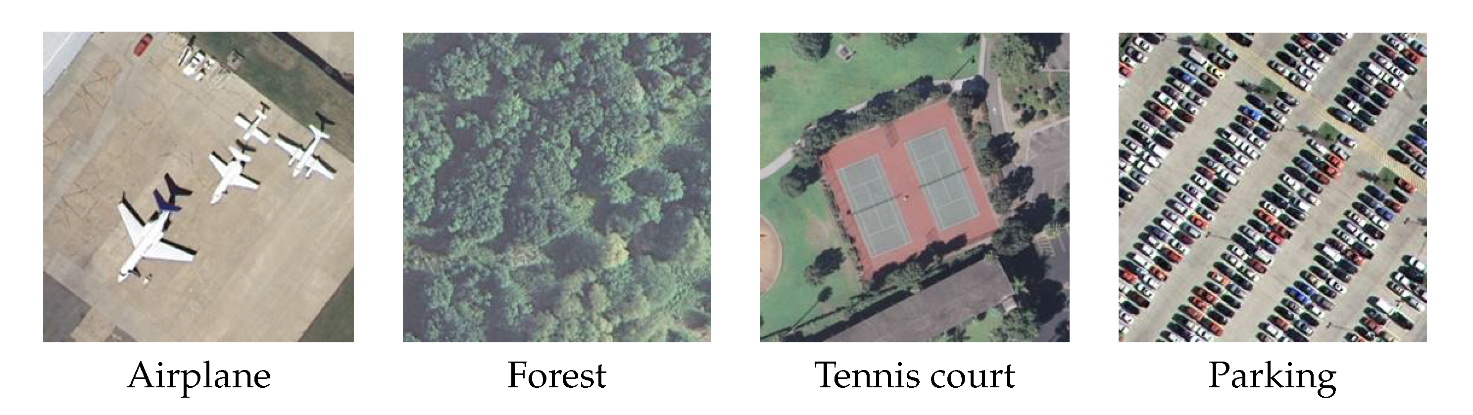
51]. This dataset is composed of 21 classes where each class contains 100 remote sensing images of dimension 256 × 256 pixels. Figure 3 shows some examples of the UC Merced dataset image classes. In order to prove the efficiency of the proposed approaches in challenging conditions, only a small set of p = 10 % images is retrained for training for all experiments and the remaining images are used for testing. Classification results are evaluated in terms of overall accuracy averaged on five runs.
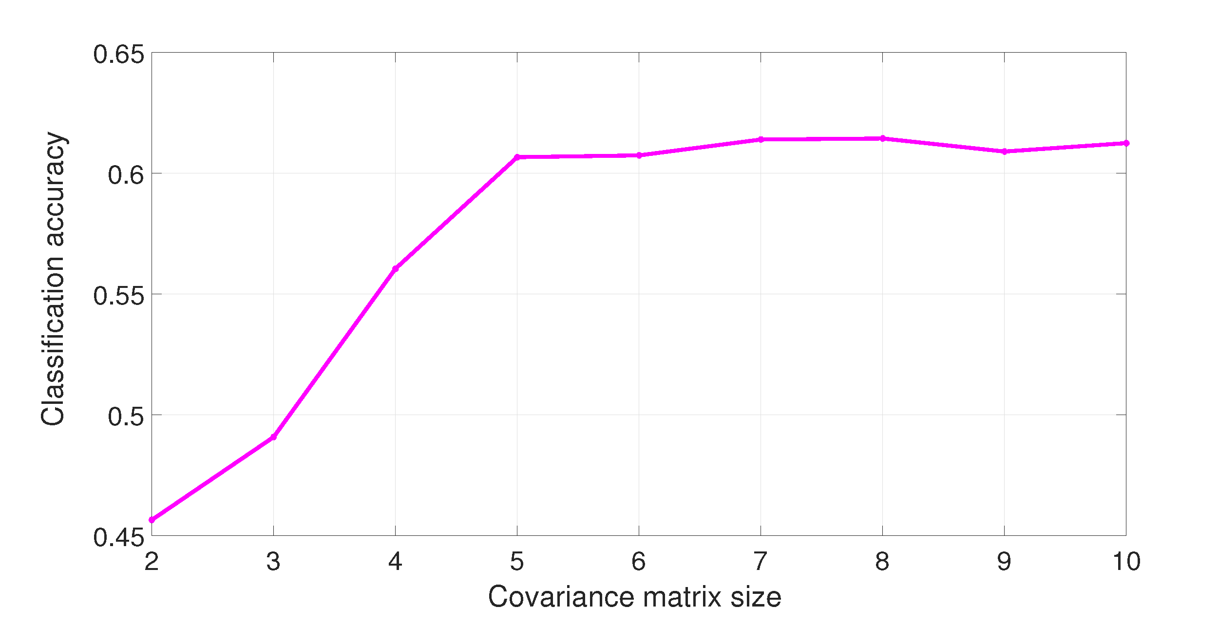
Figure 4 draws the evolution of the classification accuracy of the proposed Hybrid LE FV approach for the first convolutional layer as a function of the dimension d of the covariance matrix. Here, the number of GMM components is fixed equal to 30. The dimension d is the number of selected principal components. If d is too small, a low number of principal components is retained. All the variability is not well explained, which leads to low classification accuracy. When d increases, more variability is explained, and the classification performance also increases. But after a certain value ( d = 5 in our experiments), the variance gain is not so important and the classification performance remains quite stable. Hence, it is recommended to consider a covariance matrix size greater than a value of d = 5 .
To evaluate the sensitivity of the proposed approach to number of GMM components, Table 1 shows the classification accuracy using three values of K in the GMM model. As observed, the approach isn’t sensitive to the codebook dimension.

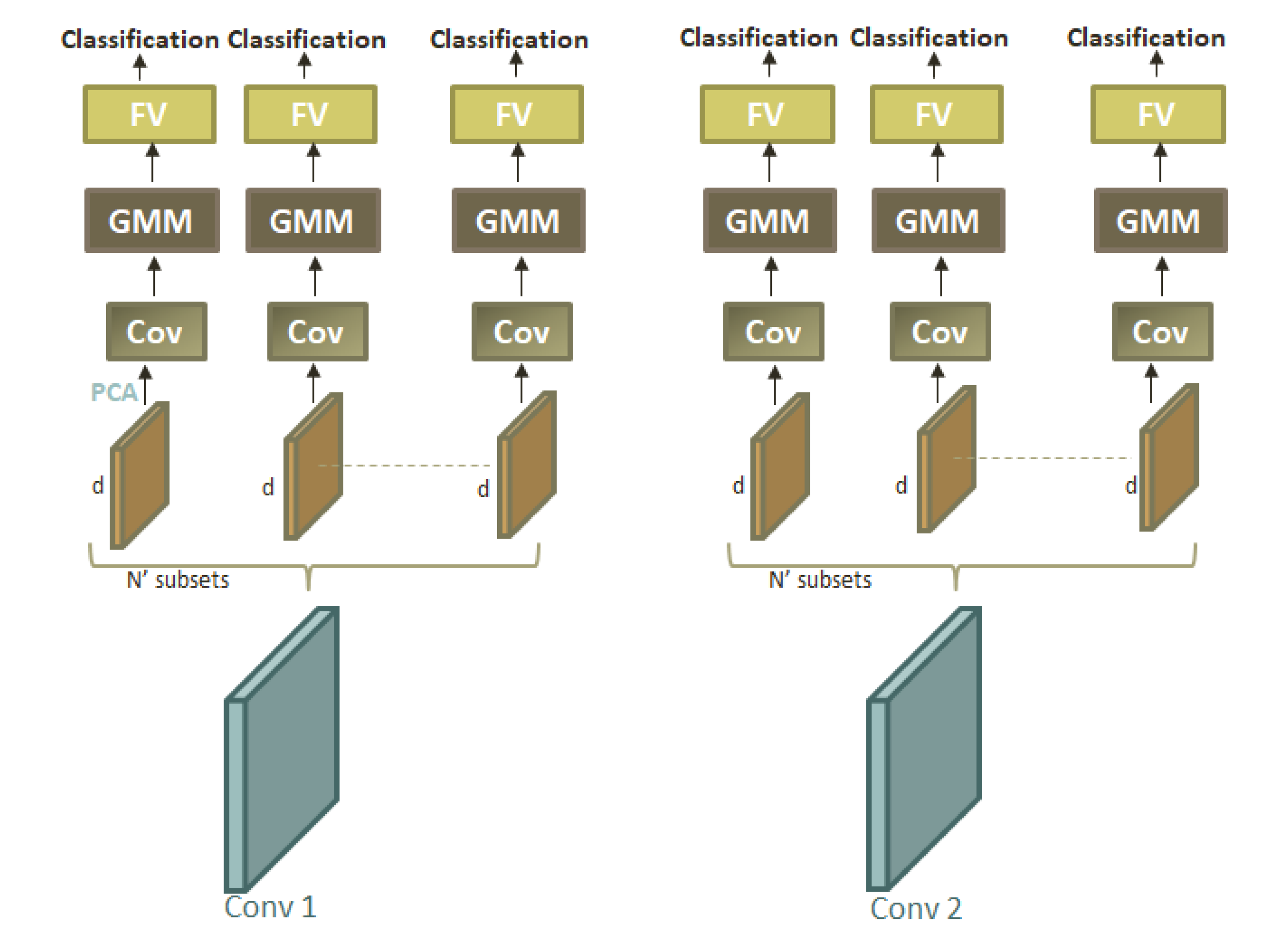
3.2. Ensemble Hybrid Log-Euclidean Fisher Vector (Ens. Hybrid LE FV)

In machine learning, ensemble learning strategies have become more and more popular [52,53]. They rely on the combination of multiple weak classifiers to form a stronger one, hence allowing improvements to the classification performance. Inspired by this idea, we introduce an ensemble learning approach for the hybrid log-Euclidean Fisher vector presented in the previous subsection. The workflow of this method named “Ens. Hybrid LE FV”, is shown in Figure 5. As observed, for each convolutional layer (conv 1 and/or conv 2), N subsets are considered. For each subset, d feature maps are randomly selected with replacement. Then, the hybrid log-Euclidean Fisher vector presented before is applied to obtain a decision for this subset. In the end, a majority vote over these decisions is considered to obtain the final prediction.
A first experiment is conducted in order to evaluate the sensitivity of the proposed approach. This consists of evaluating the influence of the number of subsets N . Table 2 shows the classification accuracy of the “Ens. Hybrid LE FV” strategy regarding the first convolutional layer of Vgg-vd-16 model. Five values of N are experimented (5, 7, 9, 11, and 13) for p = 10 % of training images of the UC Merced dataset.
One can observe that results remain quite stable of the considered subsets N . For further experiments, the number of subsets N will be fixed to 7. Table 3 highlights the classification results obtained on the UC Merced dataset for the first (conv 1) and second (conv 2) convolutional layers of vgg-vd-16 network. The proposed ensemble learning approach, “Ens. Hybrid LE FV”, is compared to two closely related state-of-the-art strategies. The first one, named “Hybrid FV”, consists of encoding the output of the convolutional layers with FV [20]. Note that this approach considers only first-order statistics. The second one, named “Hybrid LE FV” is the one presented in Section 3.1. It exploits second-order statistics but not in an ensemble learning approach [28].
As observed in Table 3, the benefit of exploiting second-order statistics is clearly demonstrated for the first and second CNN convolutional layers. A significant gain of 20% to 25% is reported for the proposed “Hybrid LE FV” and “Ens. Hybrid LE FV” methods compared to the conventional “Hybrid FV” approach. In addition, for these first two layers, a significant gain is observed when exploiting an ensemble learning strategy compared to the use of a single classifier. In this approach, only covariance matrices computed on the first layers of a CNN have been encoded with the LE FV. Indeed, as the deepest convolutional layers of the 
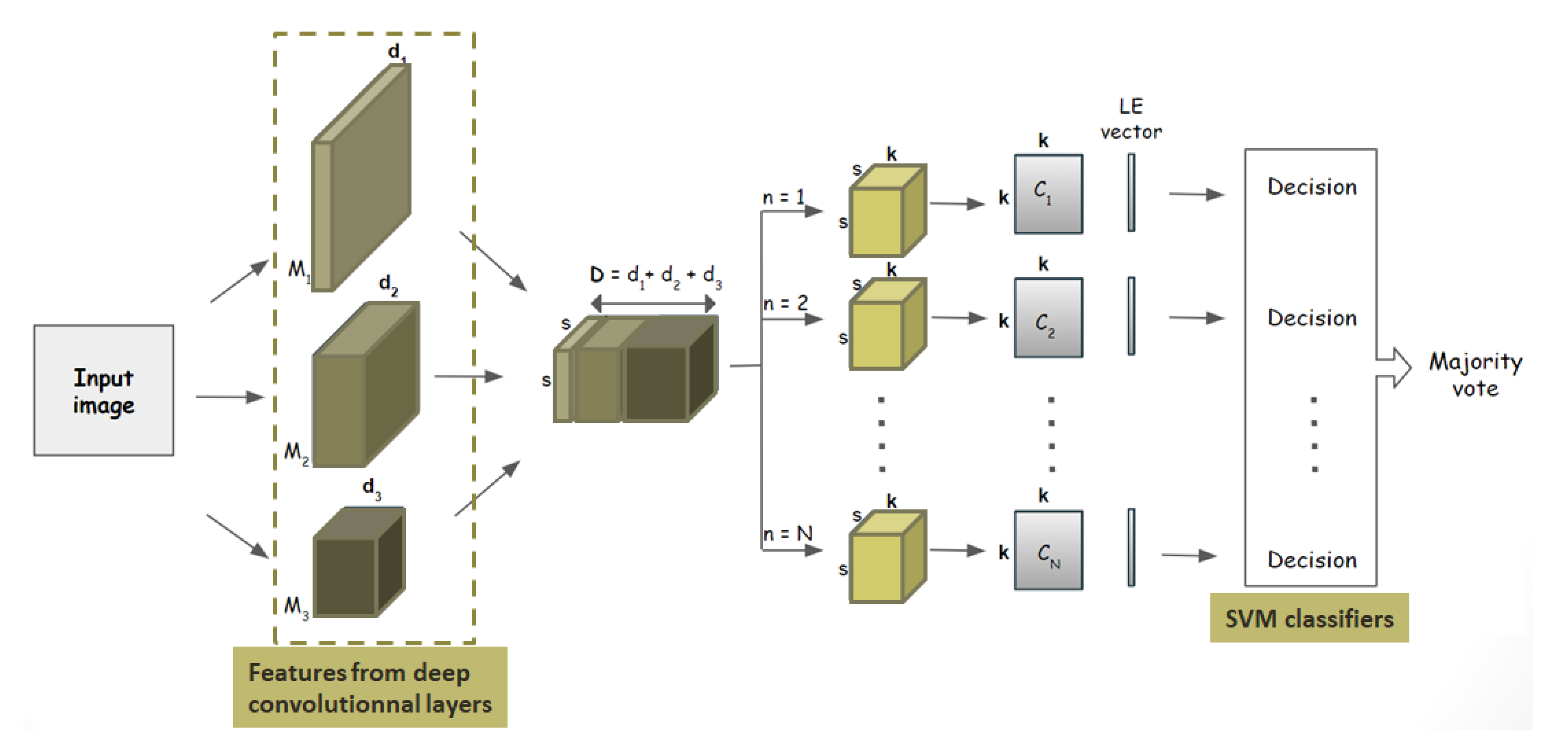
vgg-vd-16 network are of relatively small spatial dimensions, it is irrelevant to compute a sufficient number of region covariance matrices. Nevertheless, the deepest layers may provide useful features for the classification. To alleviate this issue, instead of considering a local approach, the covariance matrix will be computed globally for the deepest feature maps. For that, Section 4 introduces our ensemble learning approach based on a global covariance pooling of CNN features [44].

4. Global Covariance Pooling: Ensemble Learning Based on Covariance Pooling of CNN Features (ELCP)

4.1. Main Motivations and Global Principle

Willing to exploit second-order statistics on deep convolutional layers of a CNN, He et al., have proposed in [35] a strategy named multilayer stacked covariance pooling (MSCP). The originality lies in the replacement of the usual first-order pooling (i.e., average or max pooling) in a CNN by a second-order pooling (i.e., covariance pooling). Note also that, in contrast with the ensemble hybrid LE FV method introduced in Section 3.2, where each layer is presented by a set of covariance matrices computed locally on the feature maps, a single covariance matrix is computed for MSCP, which can significantly speed up the computation time. MSCP has successfully been validated for remote sensing scene classification, but it suffers from two main drawbacks. First, it does not exploit an ensemble learning approach. A single decision is obtained at the end. Second, and probably the main drawback, is that the averaging operator used before the covariance pooling may lead to a not well-conditioned covariance matrix. There is no practical reason that the average descriptor obtained on one subset should be different from the one calculated on another subset. To overcome these problems, we have introduced in [44] a novel hybrid approach named ELCP, which consists of an ensemble learning approach based on covariance pooling of CNN features. The global principle is shown in Figure 6.
First, the features M 1 , M 2 and M 3 produced by three deep convolutional layers ( c o n v 3 3 , c o n v 4 3 and c o n v 5 3 ) are considered. Commonly, CNN layers have different spatial dimensions. For example, for the vgg-vd-16 model, dimensions are M 1 R 56 × 56 × 256 , M 2 R 28 × 28 × 512 and M 3 R 14 × 14 × 512 . A downsampling to the smallest spatial dimension is performed using a bilinear interpolation to stack the feature maps of these latter layers. Furthermore, for each image, an ensemble learning approach is considered where the stacked feature maps generated by the convolutional layers are split into N subsets of k features each. This splitting is achieved by random sampling with replacement. Then, for each subset n, a covariance pooling strategy is adopted. It consists in computing the k × k covariance matrix C n . The log-Euclidean framework presented in Section 2 is then adopted to represent C n in the tangent plane of the identity matrix by c n T I d according to Equation (4). Then, for each subset, these log-Euclidean vectors are fed to a base linear SVM classifier allowing them to obtain a decision. The final prediction is obtained as the most represented decision among the N subsets.
For more details on the sensitivity of ELCP to its input parameters, the interested reader is referred to [44]. Since the classification results for this method are stable and not so sensitive to parameter tuning, the number of subsets N and the number of feature maps k per subset retained in the following will, respectively be equal to 20 and 170 as suggested on [44].

4.2. Experimental Results

This subsection presents some comparison of the proposed ELCP approach with some standard and recent state-of-the-art approaches on the UC Merced dataset where 10 % ( p = 10 % ) of the samples are used for training. A first approach is the FV encoding of handcrafted SIFT features (FV SIFT) [5]. The next approaches are transfer learning methods based on the vgg-vd 16 pre-trained CNN model on the ImageNet dataset. A fine-tuning of this model is first considered (CNN (vgg-vd-16 fine-tuned)). For that, the convolutional layers are frozen, and a fully connected layer is added and trained on the UC Merced dataset. The second transfer learning approach (vgg-vd-16 feat. extraction + SVM) consists in considering the CNN model as a feature extractor. CNN features are then fed to an SVM classifier. Finally, the two second-order based methods, namely MSCP and the proposed ELCP approaches, are compared. Table 4 summarizes the classification results obtained for these five methods.
As observed in Table 4, several conclusions can be drawn. First, deep learning-based methods outperform traditional handcrafted based ones. Second, since a low number of samples is used for training in this experiment, a fine-tuning strategy does not provide the best results. It is better to consider a pre-trained CNN model as the feature extractor [43,55]. A gain of more than 20 % is observed between these strategies. Third, among the transfer learning strategies based on feature extraction, methods exploiting second-order statistics of CNN features (MSCP and ELCP) outperform the first-order one. Fourth, by exploiting an ensemble strategy, the proposed ELCP significantly outperform MSCP. A gain of about 2 % is observed.

5. Decision Combination

5.1. Comparison Between Ens. Hybrid LE FV and ELCP Methods

Two transfer learning approaches have been presented, namely Ens. Hybrid LE FV in Section 3 and ELCP in Section 4. There are some similarities between these two methods. Both are based on covariance pooling of CNN features, where the log-Euclidean framework presented in Section 2 is adopted. They also exploit an ensemble learning approach. The main difference is that second-order statistics of CNN feature maps are computed locally on the first layers for Ens. Hybrid LE FV, while they are computed globally on deeper layers for ELCP. Unsurprisingly, as observed in Table 3 and Table 4, ELCP has better classification performance than Ens. Hybrid LE FV since it exploits deeper CNN features. A gain of 26 % and 20 % are, respectively, observed for ELCP compared to the first and second layers of Ens. Hybrid LE FV. However, by looking closely at the classification results, it is possible to find some images that are well classified only by Ens. Hybrid LE FV, whereas ELCP fails at this task. Figure 7 shows some images from the UC Merced dataset with the predicted class by these methods. As observed, the first two ones are correctly classified only by Ens. Hybrid LE FV, while for the last two ones, only ELCP succeeds. By taking a closer look at these results, it can be observed that, for the first two images which belong to the baseball diamond class, ELCP seems to focus on the road and building located at the top of the images. Since it exploits deeper layers of a CNN, ELCP learns high-level features that are not so useful for these particular images. Low-level features are sufficient for these images. On the other hand, the third and fourth images of Figure 7, are well classified only by ELCP; since the scene is more complex, high-level features are helpful. It therefore seems natural to combine Ens. Hybrid LE FV and ELCP in order to benefit from both low-level and high-level features. Based on the principle of the most diverse ensembles, the next subsection presents a simple fusion scheme between these two approaches.

5.2. Fusion Scheme

As previously mentioned, Ens. Hybrid LE FV and ELCP methods can be complementary since they exploit features extracted from different layers. To benefit from both strategies, many multiple classifier systems have been proposed in the literature, such as dynamic selection techniques [56]. However, the goal here is not to provide the best way to combine Ens. Hybrid LE FV and ELCP methods but rather to show the potential of their fusion. For that, we will focus on two standard and straightforward strategies. The first one, denoted as Fusion Ens. Hybrid LE FV-ELCP (MV), is simply a majority vote on the decision obtained on the output of each subset of Ens. Hybrid LE FV and ELCP. The second one, denoted as Fusion Ens. Hybrid LE FV-ELCP (MDE+MV), selects the most diverse ensembles (MDE) from these methods according to the disagreement diversity measure and greedy optimization [53]. In the end, a majority vote on these selected ensembles is performed. Table 5 summarizes the main results obtained on the UC Merced dataset for the original Ens. Hybrid LE FV and ELCP approaches and their fused versions. As observed, since the classification performances are significantly better for ELCP than Ens. Hybrid LE FV, a simple majority vote is not adapted. The accuracy of this fusion scheme (MV) is profoundly affected by the Ens. Hybrid LE FV scheme. However, by selecting the most diverse ensembles (MDE+MV), a slight gain is observed compared to ELCP, illustrating its potential.

6. Experiments on Other Datasets

In this section, experiments on other remote sensing scene classification datasets are conducted to evaluate the effectiveness of the proposed approach. For that, the SIRI-WHU Google dataset [57], the AID dataset and two real texture datasets, respectively, for maritime pine forest and on oyster fields [58,59] were tested. In order to prove the efficiency of the proposed approaches in challenging conditions, only 10 % of images were considered for training.
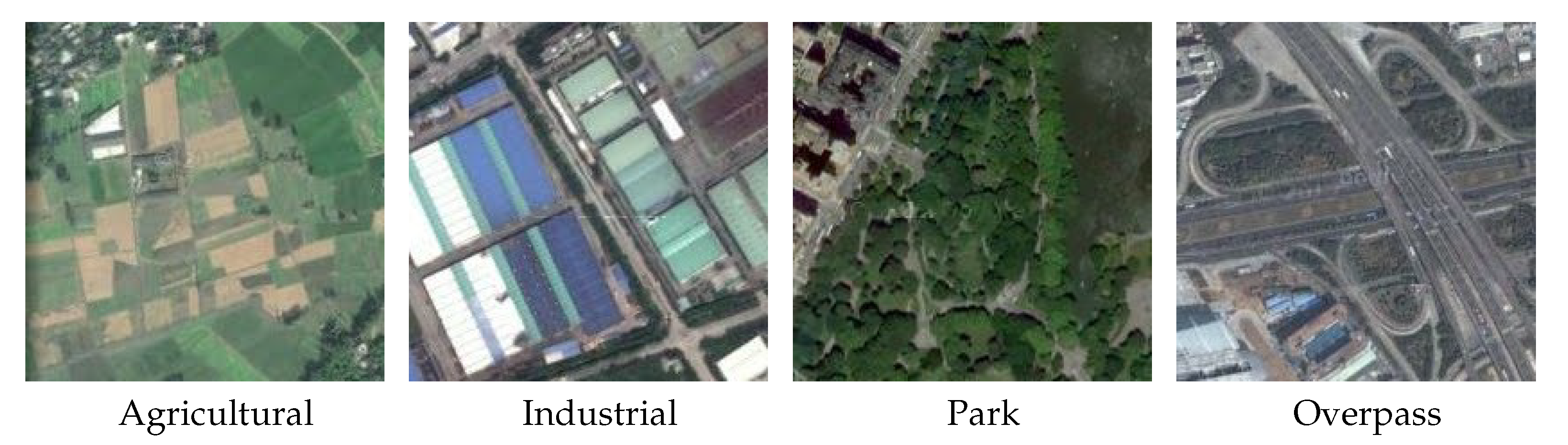
SIRI-WHU:
This is a 12-class Google image dataset, where each class contains 200 images of 200 × 200 pixels, with a 2-m spatial resolution. This dataset was acquired from Google Earth and covers urban areas in China. Figure 8 shows some image examples of the dataset.
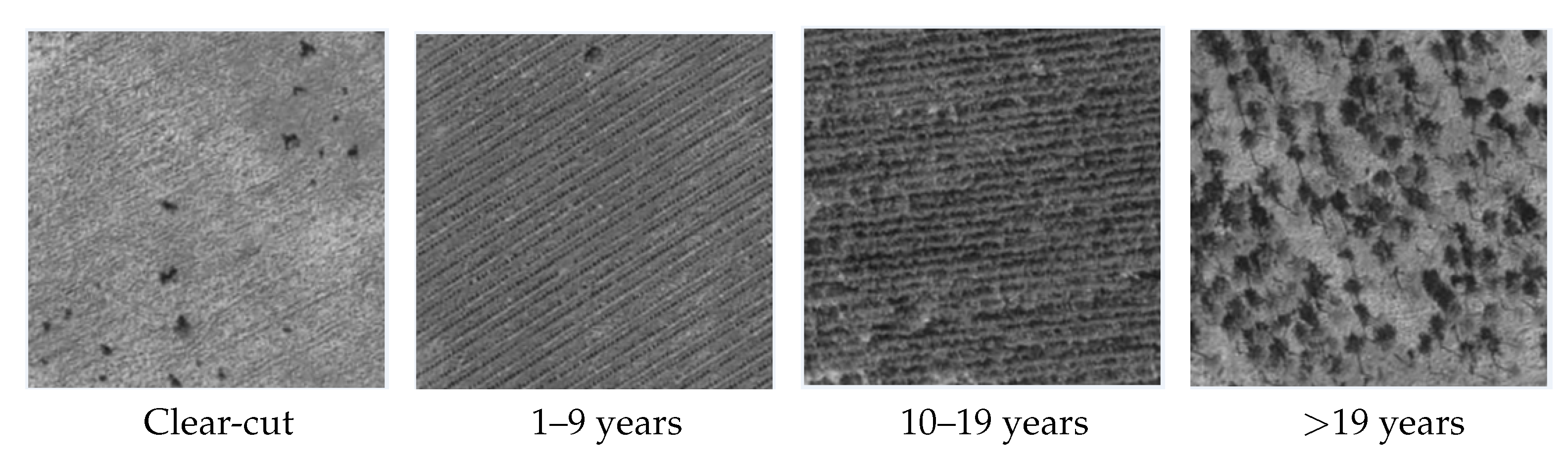
Maritime pine forest:
This dataset comprises four classes of panchromatic Pléiades satellite images with a spatial resolution of 50 cm, which represent a monitoring of growing maritime pine tree stands. Figure 9 illustrates one image from each age class.
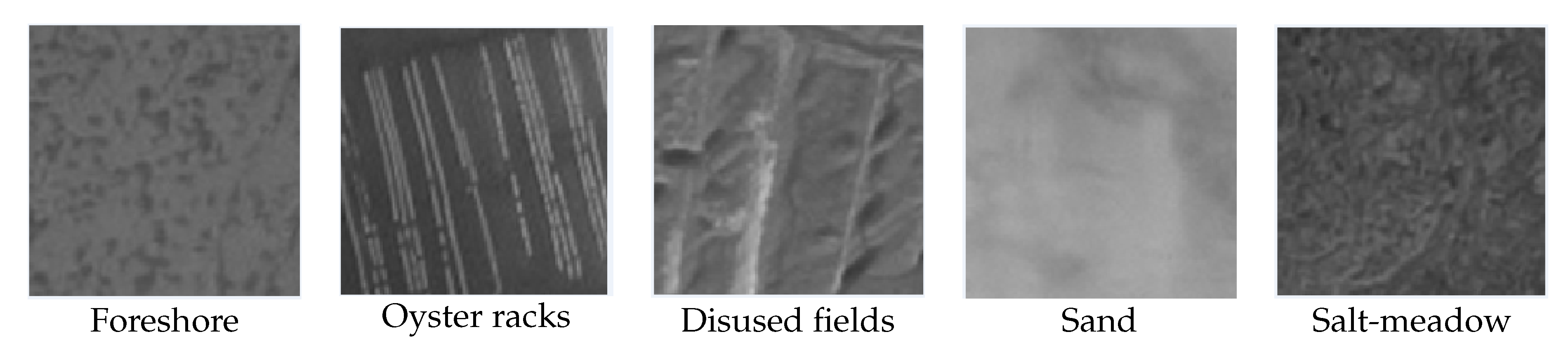
Oyster racks:
This five-class dataset is also formed from panchromatic Pléiades satellite high-resolution images. It is comprised, in particular, of images representing cultivated oyster racks and abandoned fields. Figure 10 shows one image of each class of the oyster dataset.
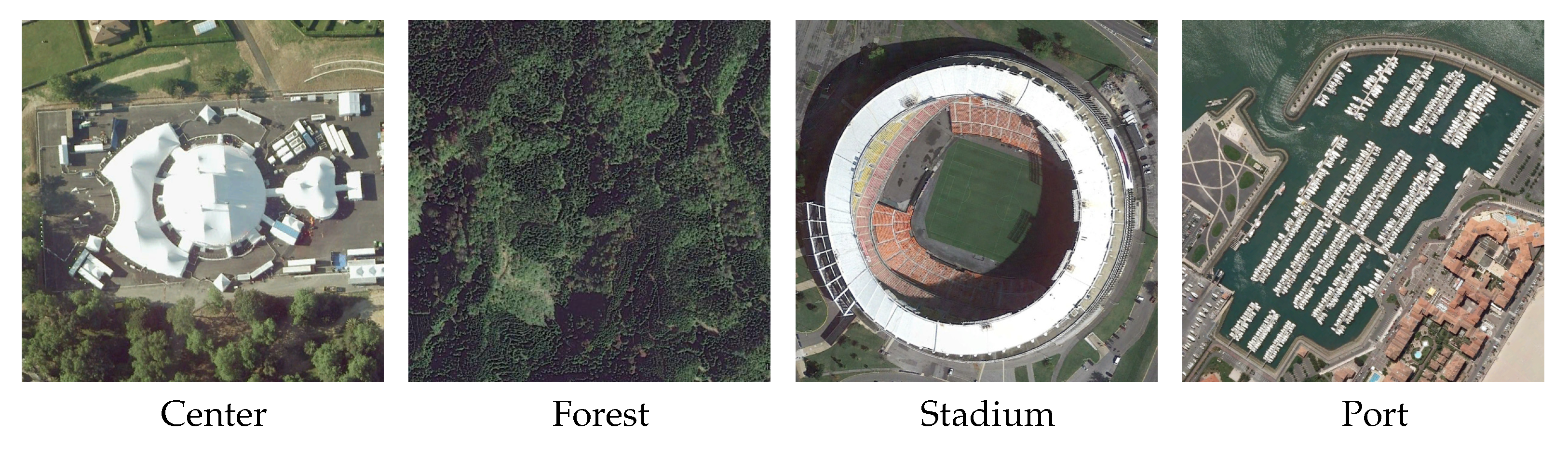
AID:
This dataset contains 10,000 aerial images of dimension 600 × 600 pixels partitioned into 30 classes, with a 2-m spatial resolution. Figure 11 illustrates some dataset images.
Table 6 below summarizes the main characteristics of the considered datasets.
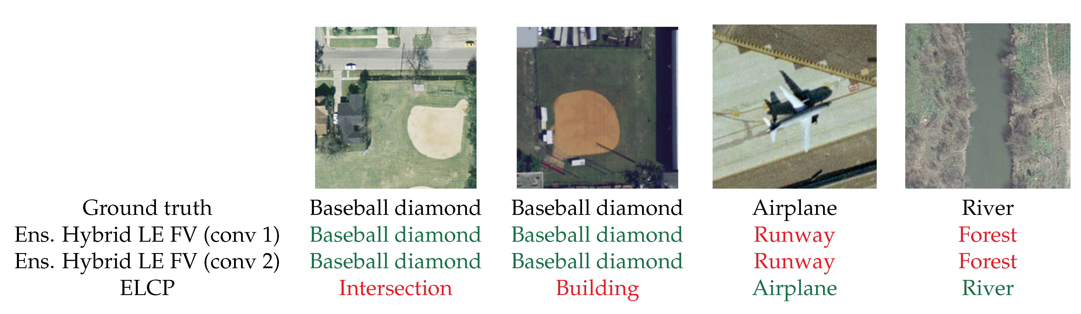
The experiments carried out consist of validating the proposed fusion scheme of the two proposed ensemble learning approaches, namely the Fusion Ens. Hybrid LE FV-ELCP (MDE+MV) strategy.
Table 7 summarizes the main results. As observed, a similar conclusion can be draw from these four datasets. Firstly, the ELCP approach performs better than Ens. Hybrid LE FV on first and second CNN convolutional layers due to the considered convolutional layer depth. This clearly illustrates the interest of exploiting deep feature maps from CNN model, which characterizes high-level features compared to the first ones. Secondly, a similar conclusion can be drawn to the one obtained from the UC Merced dataset: the fusion of both local and global second-order statistics computation strategies permits enhancing classification performance, which illustrates the multi-layer fusion efficiency.

7. Conclusions

This paper has introduced a new transfer learning approach based on the covariance pooling of CNN features maps. The proposed ensemble learning approach consists of the fusion of two hybrid architectures. These two strategies use features extracted from models pre-trained on the ImageNet dataset. The former exploits low-level features extracted from the first and second layers. It consists of the log-Euclidean Fisher vector encoding of region covariance matrices computed locally, while the latter uses high-level features issued from deeper layers that are pooled together by computing their covariance matrix. These two strategies share many similarities. They are ensemble learning strategies based on the log-Euclidean representation of the covariance matrix of these CNN features. However, since they exploit feature maps extracted from different layers, they can be considered as complementary. These two ensemble learning strategies were hence combined together using the strategy of the most diverse ensembles. The proposed approach was then successfully validated on various dataset for remote sensing scene classification, illustrating its efficiency and the interest of second-order features. Competitive results have been obtained, with a gain of about 1 to 2 % in term of overall accuracy, compared to the recent state-of-the-art.
Since the proposed approach is based on covariance pooling of CNN features, any deep convolutional neural network can be used as backbone. Future works will concerns the adaptation of the proposed strategy to multispectral or hyperspectral images dataset, where a CNN will be used for this kind of data [60,61].

Author Contributions

Conceptualization, S.A., L.B. and Y.B.; Formal analysis, S.A. and L.B.; Funding acquisition, L.B., J.X. and C.G.; Methodology, S.A., L.B., J.X., Y.B. and C.G.; Project administration, C.G.; Software, S.A., L.B. and J.X.; Supervision, L.B., Y.B. and C.G.; Validation, L.B., J.X. and Y.B.; Writing—original draft, S.A. and L.B.; Writing—review and editing, S.A., L.B., J.X., Y.B. and C.G. All authors have read and agreed to the published version of the manuscript.

Funding

This work was financially supported by the “PHC Sakura” program (project number 45095SK), implemented by the French Ministry for Europe and Foreign Affairs, the French Ministry of Higher Education, Research and Innovation and the Japan Society for Promotion of Science. The authors would also acknowledge the financial support of Bordeaux Sciences Agro and the Regional Council of Nouvelle Aquitaine, France.

Acknowledgments

The authors would like to thank S. D. Newsam and G. Xia for providing the UC Merced and AID datasets. The authors would also like to thank Centre National d’Etudes Spatiales (CNES, France) and its Thematic Users Commissioning Team for providing the Pléiades data and the Telespazio and Alliance Forêt-Bois for authorizing the use of their stand age reference data. The authors would also like to thank the reviewers for their comments and corrections that helped us to improve this paper.

Conflicts of Interest

The authors declare no conflict of interest.

References

  1. Sivic, J.; Russell, B.C.; Efros, A.A.; Zisserman, A.; Freeman, W.T. Discovering objects and their location in images. In Proceedings of the Tenth IEEE International Conference on Computer Vision (ICCV’05), Beijing, China, 17–21 October 2005; pp. 370–377, volume 1. [Google Scholar] [CrossRef] [Green Version]
  2. Jégou, H.; Douze, M.; Schmid, C.; Pérez, P. Aggregating local descriptors into a compact image representation. In Proceedings of the 2010 IEEE Computer Society Conference on Computer Vision and Pattern Recognition, San Francisco, CA, USA, 13–18 June 2010; pp. 3304–3311. [Google Scholar] [CrossRef] [Green Version]
  3. Arandjelović, R.; Zisserman, A. All about VLAD. In Proceedings of the IEEE Conference on Computer Vision and Pattern Recognition, Portland, OR, USA, 23–28 June 2013; pp. 1578–1585. [Google Scholar]
  4. Perronnin, F.; Dance, C. Fisher kernels on visual vocabularies for image categorization. In Proceedings of the IEEE Conference on Computer Vision and Pattern Recognition, Minneapolis, MN, USA, 17–22 June 2007; pp. 1–8. [Google Scholar]
  5. Perronnin, F.; Sánchez, J.; Mensink, T. Improving the Fisher kernel for large-scale image classification. In Proceedings of the 11th European Conference on Computer Vision: Part IV, Heraklion, Greece, 5–11 September 2010; Springer-Verlag: Berlin/Heidelberg, Germany, 2010; pp. 143–156. [Google Scholar]
  6. Perronnin, F.; Liu, Y.; Sánchez, J.; Poirier, H. Large-scale image retrieval with compressed Fisher vectors. In Proceedings of the The Twenty-Third IEEE Conference on Computer Vision and Pattern Recognition, San Francisco, CA, USA, 13–18 June 2010; pp. 3384–3391. [Google Scholar] [CrossRef]
  7. Douze, M.; Ramisa, A.; Schmid, C. Combining attributes and Fisher vectors for efficient image retrieval. In Proceedings of the IEEE Conference on Computer Vision and Pattern Recognition, Providence, RI, USA, 20–25 June 2011; pp. 745–752. [Google Scholar] [CrossRef] [Green Version]
  8. Sánchez, J.; Perronnin, F.; Mensink, T.; Verbeek, J. Image classification with the Fisher vector: Theory and practice. Int. J. Comput. Vis. 2013, 105, 222–245. [Google Scholar] [CrossRef]
  9. Salton, G.; Buckley, C. Term-weighting approaches in automatic text retrieval. Inf. Process. Manag. 1988, 24, 513–523. [Google Scholar] [CrossRef] [Green Version]
  10. Faraki, M.; Harandi, M.T.; Porikli, F. More about VLAD: A leap from Euclidean to Riemannian manifolds. In Proceedings of the IEEE Conference on Computer Vision and Pattern Recognition, Boston, MA, USA, 7–12 June 2015; pp. 4951–4960. [Google Scholar] [CrossRef]
  11. Kriegeskorte, N. Deep neural networks: A new framework for modelling biological vision and brain information processing. bioRxiv 2015. [Google Scholar] [CrossRef]
  12. Le Cun, Y.; Boser, B.E.; Denker, J.S.; Henderson, D.; Howard, R.E.; Hubbard, W.E.; Jackel, L.D. Handwritten digit recognition with a back-propagation network. In Advances in Neural Information Processing Systems 2; Touretzky, D.S., Ed.; Morgan-Kaufmann: Berlington, MA, USA, 1990; pp. 396–404. [Google Scholar]
  13. Krizhevsky, A.; Sutskever, I.; Hinton, G.E. ImageNet classification with deep convolutional neural networks. In Proceedings of the 25th International Conference on Neural Information Processing Systems (NIPS’12), Lake Tahoe, NV, USA, 3–6 December 2012; Curran Associates Inc.: Red Hook, NY, USA, 2012; Volume 1, pp. 1097–1105. [Google Scholar]
  14. Perronnin, F.; Larlus, D. Fisher vectors meet neural networks: A hybrid classification architecture. In Proceedings of the 2015 IEEE Conference on Computer Vision and Pattern Recognition (CVPR), Boston, MA, USA, 7–12 June 2015; pp. 3743–3752. [Google Scholar] [CrossRef]
  15. Simonyan, K.; Vedaldi, A.; Zisserman, A. Deep Fisher networks for large-scale image classification. In Proceedings of the 26th International Conference on Neural Information Processing Systems (NIPS’13), Lake Tahoe, NV, USA, 5–10 December 2013; Curran Associates Inc.: Red Hook, NY, USA, 2013; Volume 1, pp. 163–171. [Google Scholar]
  16. Arandjelovic, R.; Gronát, P.; Torii, A.; Pajdla, T.; Sivic, J. NetVLAD: CNN architecture for weakly supervised place recognition. In Proceedings of the IEEE Conference on Computer Vision and Pattern Recognition, Las Vegas, NV, USA, 27–30 June 2016. [Google Scholar]
  17. Ng, J.; Yang, F.; Davis, L.S. Exploiting local features from deep networks for image retrieval. In Proceedings of the 2015 IEEE Conference on Computer Vision and Pattern Recognition Workshops (CVPRW), Boston, MA, USA, 7–12 June 2015. [Google Scholar]
  18. Cimpoi, M.; Maji, S.; Kokkinos, I.; Vedaldi, A. Deep filter banks for texture recognition, description, and segmentation. Int. J. Comput. Vis. 2016, 118, 65–94. [Google Scholar] [CrossRef] [PubMed] [Green Version]
  19. Diba, A.; Pazandeh, A.M.; Gool, L.V. Deep visual words: Improved Fisher vector for image classification. In Proceedings of the 2017 Fifteenth IAPR International Conference on Machine Vision Applications (MVA), Nagoya, Japan, 8–12 May 2017; pp. 186–189. [Google Scholar] [CrossRef]
  20. Li, E.; Xia, J.; Du, P.; Lin, C.; Samat, A. Integrating multilayer features of convolutional neural networks for remote sensing scene classification. IEEE Trans. Geosci. Remote Sens. 2017, 55, 5653–5665. [Google Scholar] [CrossRef]
  21. Julesz, B.B.; Gilbert, E.N.; Shepp, L.A.; Frisch, H.L. Perception. Inability of humans to discriminate between visual textures that agree in second-order statistics-revisited. Perception 1973, 2, 391–405. [Google Scholar] [CrossRef]
  22. Barachant, A.; Bonnet, S.; Congedo, M.; Jutten, C. Classification of covariance matrices using a Riemannian-based kernel for BCI applications. NeuroComputing 2013, 112, 172–178. [Google Scholar] [CrossRef] [Green Version]
  23. Said, S.; Bombrun, L.; Berthoumieu, Y. Texture classification using Rao’s distance on the space of covariance matrices. In Proceedings of the Geometric Science of Information, Palaiseau, France, 28–30 October 2015; Volume 9389, pp. 371–378. [Google Scholar] [CrossRef] [Green Version]
  24. Kong, S.; Fowlkes, C. Low-rank Bilinear Pooling for Fine-Grained Classification. arXiv 2016, arXiv:cs.CV/1611.05109. [Google Scholar]
  25. Yuan, C.; Hu, W.; Li, X.; Maybank, S.; Luo, G. Human action recognition under log-Euclidean Riemannian metric. In Proceedings of the Computer Vision—ACCV 2009: 9th Asian Conference on Computer Vision, Xi’an, China, 23–27 September 2009; pp. 343–353. [Google Scholar] [CrossRef]
  26. Faraki, M.; Palhang, M.; Sanderson, C. Log-Euclidean bag of words for human action recognition. IET Comput. Vis. 2015, 9, 331–339. [Google Scholar] [CrossRef] [Green Version]
  27. Faraki, M.; Harandi, M.T.; Wiliem, A.; Lovell, B.C. Fisher tensors for classifying human epithelial cells. Pattern Recognit. 2014, 47, 2348–2359. [Google Scholar] [CrossRef]
  28. Akodad, S.; Bombrun, L.; Yaacoub, C.; Berthoumieu, Y.; Germain, C. Image classification based on log-Euclidean Fisher Vectors for covariance matrix descriptors. In Proceedings of the International Conference on Image Processing Theory, Tools and Applications (IPTA), Xi’an, China, 7–10 November 2018. [Google Scholar]
  29. Ilea, I.; Bombrun, L.; Germain, C.; Terebes, R.; Borda, M.; Berthoumieu, Y. Texture image classification with Riemannian Fisher vectors. In Proceedings of the IEEE International Conference on Image Processing, Phoenix, AZ, USA, 25–28 September 2016; pp. 3543–3547. [Google Scholar]
  30. Ilea, I.; Bombrun, L.; Said, S.; Berthoumieu, Y. Covariance matrices encoding based on the log-Euclidean and affine invariant Riemannian metrics. In Proceedings of the IEEE/CVF Conference on Computer Vision and Pattern Recognition Workshops (CVPRW), Salt Lake City, UT, USA, 18–22 June 2018; pp. 506–515. [Google Scholar] [CrossRef] [Green Version]
  31. Ilea, I.; Bombrun, L.; Said, S.; Berthoumieu, Y. Fisher vector coding for covariance matrix descriptors based on the log-Euclidean and affine invariant Riemannian metrics. J. Imaging 2018, 4, 85. [Google Scholar] [CrossRef] [Green Version]
  32. Arsigny, V.; Fillard, P.; Pennec, X.; Ayache, N. Log-Euclidean metrics for fast and simple calculus on diffusion tensors. Magn. Reson. Med. 2006, 56, 411–421. [Google Scholar] [CrossRef] [PubMed]
  33. Ionescu, C.; Vantzos, O.; Sminchisescu, C. Matrix backpropagation for deep networks with structured layers. In Proceedings of the IEEE International Conference on Computer Vision (ICCV), Santiago, Chile, 7–13 December 2015; pp. 2965–2973. [Google Scholar]
  34. Cai, S.; Zuo, W.; Zhang, L. Higher-Order Integration of Hierarchical Convolutional Activations for Fine-Grained Visual Categorization. In Proceedings of the 2017 IEEE International Conference on Computer Vision (ICCV), Venice, Italy, 22–29 October 2017; pp. 511–520. [Google Scholar]
  35. He, N.; Fang, L.; Li, S.; Plaza, A.; Plaza, J. Remote sensing scene classification using multilayer stacked covariance pooling. IEEE Trans. Geosci. Remote Sens. 2018, 56, 6899–6910. [Google Scholar] [CrossRef]
  36. Huang, Z.; Gool, L.V. A Riemannian network for SPD matrix learning. In Proceedings of the AAAI Conference on Artificial Intelligence, San Francisco, CA, USA, 4–9 February 2017; pp. 2036–2042. [Google Scholar]
  37. Yu, K.; Salzmann, M. Second-order convolutional neural networks. arXiv 2017, arXiv:1703.06817. [Google Scholar]
  38. Acharya, D.; Huang, Z.; Paudel, D.P.; Van Gool, L. Covariance pooling for facial expression recognition. arXiv 2018, arXiv:1805.04855. [Google Scholar]
  39. Gao, Z.; Xie, J.; Wang, Q.; Li, P. Global second-order pooling convolutional networks. In Proceedings of the 2019 IEEE/CVF Conference on Computer Vision and Pattern Recognition (CVPR), Long Beach, CA, USA, 15–20 June 2019; pp. 3019–3028. [Google Scholar]
  40. He, N.; Fang, L.; Li, S.; Plaza, J.; Plaza, A. Skip-connected covariance network for remote sensing scene classification. IEEE Trans. Neural Netw. Learn. Syst. 2020, 31, 1461–1474. [Google Scholar] [CrossRef] [Green Version]
  41. Sumbul, G.; Charfuelan, M.; Demir, B.; Markl, V. BigEarthNet: A large-scale benchmark archive for remote sensing image understanding. In Proceedings of the IEEE International Geoscience and Remote Sensing Symposium, Yokohama, Japan, 28 July–2 August 2019. [Google Scholar]
  42. Souleyman, C.; Larabi, M.; Gu, Y.; Bakhti, K.; Karoui, M.S. Very High Resolution Image Scene Classification with Capsule Network. In Proceedings of the IGARSS 2019—2019 IEEE International Geoscience and Remote Sensing Symposium, Yokohama, Japan, 28 July–2 August 2019. [Google Scholar] [CrossRef]
  43. Pires de Lima, R.; Marfurt, K. Convolutional neural network for remote-sensing scene classification: Transfer learning analysis. Remote Sens. 2019, 12, 86. [Google Scholar] [CrossRef] [Green Version]
  44. Akodad, S.; Vilfroy, S.; Bombrun, L.; Cavalcante, C.C.; Germain, C.; Berthoumieu, Y. An ensemble learning approach for the classification of remote sensing scenes based on covariance pooling of CNN features. In Proceedings of the 2019 27th European Signal Processing Conference (EUSIPCO), A Coruna, Spain, 2–6 September 2019; pp. 1–5. [Google Scholar]
  45. Rosu, R.; Donias, M.; Bombrun, L.; Said, S.; Regniers, O.; Da Costa, J.P. Structure tensor Riemannian statistical models for CBIR and classification of remote sensing images. IEEE Trans. Geosci. Remote Sens. 2017, 55, 248–260. [Google Scholar] [CrossRef]
  46. Pham, M.T.; Mercier, G.; Bombrun, L. Color Texture Image Retrieval Based on Local Extrema Features and Riemannian Distance. J. Imaging 2017, 3, 43. [Google Scholar] [CrossRef] [Green Version]
  47. Pennec, X.; Fillard, P.; Ayache, N. A Riemannian framework for tensor computing. Int. J. Comput. Vis. 2006, 66, 41–66. [Google Scholar] [CrossRef] [Green Version]
  48. Smith, S.T. Covariance, subspace, and intrinsic Cramér-Rao bounds. IEEE Trans. Signal Proces. 2005, 53, 1610–1630. [Google Scholar] [CrossRef] [Green Version]
  49. Simonyan, K.; Zisserman, A. Very deep convolutional networks for large-scale image recognition. arXiv 2014, arXiv:1409.1556. [Google Scholar]
  50. Mika, S.; Ratsch, G.; Weston, J.; Scholkopf, B.; Mullers, K.R. Fisher discriminant analysis with kernels. In Proceedings of the Neural Networks for Signal Processing IX: Proceedings of the 1999 IEEE Signal Processing Society Workshop (Cat. No.98TH8468), Madison, WI, USA, 25 August 1999; pp. 41–48. [Google Scholar] [CrossRef]
  51. Yang, Y.; Newsam, S. Bag-of-visual-words and Spatial Extensions for Land-use Classification. In Proceedings of the 18th SIGSPATIAL International Conference on Advances in Geographic Information Systems (GIS ’10), San Jose, CA, USA, 2–5 November 2010; ACM: New York, NY, USA, 2010; pp. 270–279. [Google Scholar] [CrossRef]
  52. Breiman, L. Random forests. Mach. Learn. 2001, 45, 5–32. [Google Scholar] [CrossRef] [Green Version]
  53. Kuncheva, L.I.; Whitaker, C.J. Measures of diversity in classifier ensembles and their relationship with the ensemble accuracy. Mach. Learn. 2003, 51, 181–207. [Google Scholar] [CrossRef]
  54. Chatfield, K.; Simonyan, K.; Vedaldi, A.; Zisserman, A. Return of the devil in the details: Delving deep into convolutional nets. arXiv 2014, arXiv:1405.3531. [Google Scholar]
  55. Cheng, G.; Xie, X.; Han, J.; Guo, L.; Xia, G.S. Remote sensing image scene classification meets deep learning: challenges, methods, benchmarks, and opportunities. IEEE J. Sel. Top. Appl. Earth Obs. Remote Sens. 2020, 13, 3735–3756. [Google Scholar] [CrossRef]
  56. Cruz, R.M.; Sabourin, R.; Cavalcanti, G.D. Dynamic classifier selection: Recent advances and perspectives. Inf. Fusion 2018, 41, 195–216. [Google Scholar] [CrossRef]
  57. Zhao, B.; Zhong, Y.; Xia, G.; Zhang, L. Dirichlet-derived multiple topic scene classification model for high spatial resolution remote sensing imagery. IEEE Trans. Geosci. Remote Sens. 2016, 54, 2108–2123. [Google Scholar] [CrossRef]
  58. Regniers, O.; Bombrun, L.; Guyon, D.; Samalens, J.C.; Germain, C. Wavelet-based texture features for the classification of age classes in a maritime pine forest. IEEE Geosc. Remote Sens. Lett. 2015, 12, 621–625. [Google Scholar] [CrossRef]
  59. Regniers, O.; Bombrun, L.; Lafon, V.; Germain, C. Supervised classification of very high resolution optical images using wavelet-based textural features. IEEE Trans. Geosci. Remote Sens. 2016, 54, 3722–3735. [Google Scholar] [CrossRef] [Green Version]
  60. Hu, W.; Huang, Y.; Wei, L.; Zhang, F.; Li, H. Deep Convolutional Neural Networks for Hyperspectral Image Classification. J. Sens. 2015, 2015, 258619. [Google Scholar] [CrossRef] [Green Version]
  61. Paoletti, M.; Haut, J.; Plaza, J.; Plaza, A. A new deep convolutional neural network for fast hyperspectral image classification. ISPRS J. Photogramm. Remote Sens. 2018, 145, 120–147. [Google Scholar] [CrossRef]
Figure 1. Manifold of symmetric positive definite (SPD) matrices and projection to the tangent space at M r e f .
Remotesensing 12 03292 g001
Figure 2. Principle of the proposed log-Euclidean Fisher vector encoding of region covariance matrices (Hybrid LE FV).
Remotesensing 12 03292 g002
Figure 3. Samples from the UC Merced dataset.
Remotesensing 12 03292 g003
Figure 4. Influence of dimension d of covariance matrices for Hybrid LE FV (conv 1) on the UC Merced dataset.
Remotesensing 12 03292 g004
Figure 5. Ensemble Hybrid LE FV workflow.
Remotesensing 12 03292 g005
Figure 6. Ensemble learning approach based on covariance pooling of CNN features (ELCP) workflow.
Remotesensing 12 03292 g006
Figure 7. Samples from the UC Merced dataset. Below, ground truth and class prediction by Ens. Hybrid LE FV and ELCP approaches.
Remotesensing 12 03292 g007
Figure 8. Samples from the Google image dataset of SIRI-WHU.
Remotesensing 12 03292 g008
Figure 9. Samples from the maritime pine forest dataset.
Remotesensing 12 03292 g009
Figure 10. Samples from the oyster racks dataset.
Remotesensing 12 03292 g010
Figure 11. Samples from the AID dataset.
Remotesensing 12 03292 g011
Table 1. Classification accuracy of Hybrid LE FV using three codebook dimensions K.
MethodK = 10K = 30K = 60
Hybrid LE FV (conv 1)60.5 ± 1.0%61.2 ± 0.8%61.2 ± 0.8%
Table 2. Classification accuracy of ”Ens. Hybrid LE FV" using different number of subsets N .
Method N = 5 N = 7 N = 9 N = 11 N = 13
Ens. Hybrid LE FV63.7 ± 0.6%64.0 ± 0.3%64.0 ± 0.3%63.9 ± 0.1%64.0 ± 0.5%
Table 3. Classification results on the UC Merced dataset for the first and second convolutional layers of the vgg-vd-16 network (p = 10%).
MethodConv 1Conv 2
Hybrid FV  [20]41.4 ± 0.2%43.7 ± 1.1%
Hybrid LE FV  [28]61.2 ± 0.8%65.1 ± 1.6%
Ens. Hybrid LE FV62.4 ± 0.9%68.1 ± 1.7%
Table 4. Classification performance of the proposed multi-layer architecture compared to the state-of-the-art on the UC Merced dataset (p = 10 % ).
MethodOA (Mean ± sd)
FV (SIFT)  [5]62.3 ± 1.1%
CNN (vgg-vd-16 fine-tuned)62.7 ± 1.8%
CNN (vgg-vd-16 feat. extraction + SVM)  [54]82.7 ± 0.6%
MSCP (vgg-vd-16)  [35]86.3 ± 1.0%
ELCP (vgg-vd-16)88.4 ± 1.4%
Table 5. Classification accuracy on UC Merced dataset obtained using Ens. Hybrid LE FV, ELCP and their fusion version Ens. LE FV - ELCP methods (p = 10 % ).
DatabaseMethodOA (Mean ± sd)
Ens. Hybrid LE FV (conv1)62.4 ± 0.9%
UC MercedEns. Hybrid LE FV (conv2)68.1 ± 1.7%
p = 10 % ELCP88.4 ± 1.4%
Fusion Ens. Hybrid LE FV-ELCP (MV)88.2 ± 1.2%
Fusion Ens. Hybrid LE FV-ELCP (MDE+MV)88.7 ± 1.1%
Table 6. Remote sensing scene dataset properties
DatasetResolution (m)ClassesImagesImage SizeImage Type
SIRI-WHU2122400200 × 200Aerial
Maritime pine forests0.54471256 × 256Satellite (Pléiades)
Oyster racks0.55371128 × 128Satellite (Pléiades)
AID23010,000600 × 600Aerial
Table 7. Classification accuracy on different datasets obtained using Ens. Hybrid LE FV, ELCP and their fusion version Ens. LE FV - ELCP methods ( p = 10 % ).
DatabaseMethodOA (Mean ± sd)
Ens. Hybrid LE FV (conv1)70.0 ± 0.8%
SIRI-WHUEns. Hybrid LE FV (conv2)79.1 ± 0.9%
p = 10 % ELCP88.3 ± 1.2%
Fusion Ens. Hybrid LE FV-ELCP (MDE+MV)89.9 ± 1.6%
Ens. Hybrid LE FV (conv1)86.5 ± 2.2%
Maritime pine forestEns. Hybrid LE FV (conv2)85.7 ± 0.4%
p = 10 % ELCP87.8 ± 2.3%
Fusion Ens. Hybrid LE FV-ELCP (MDE+MV)89.1 ± 1.3%
Ens. Hybrid LE FV (conv1)84. 1 ± 2.4%
Oyster racksEns. Hybrid LE FV (conv2)86.1 ± 1.1%
p = 10 % ELCP85.7 ± 1.4%
Fusion Ens. Hybrid LE FV-ELCP (MDE+MV)86.4 ± 1.4%
Ens. Hybrid LE FV (conv1)67.4 ± 0.4%
AIDEns. Hybrid LE FV (conv2)70.9 ± 0.2%
p = 10 % ELCP87.6 ± 0.2%
Fusion Ens. Hybrid LE FV-ELCP (MDE+MV)88.7 ± 0.3%

