A GA-Based Multi-View, Multi-Learner Active Learning Framework for Hyperspectral Image Classification

Abstract

This paper introduces a novel multi-view multi-learner (MVML) active learning method, in which the different views are generated by a genetic algorithm (GA). The GA-based view generation method attempts to construct diverse, sufficient, and independent views by considering both inter- and intra-view confidences. Hyperspectral data inherently owns high dimensionality, which makes it suitable for multi-view learning algorithms. Furthermore, by employing multiple learners at each view, a more accurate estimation of the underlying data distribution can be obtained. We also implemented a spectral-spatial graph-based semi-supervised learning (SSL) method as the classifier, which improved the performance of the classification task in comparison with supervised learning. The evaluation of the proposed method was based on three different benchmark hyperspectral data sets. The results were also compared with other state-of-the-art AL-SSL methods. The experimental results demonstrated the efficiency and statistically significant superiority of the proposed method. The GA-MVML AL method improved the classification performances by 16.68%, 18.37%, and 15.1% for different data sets after 40 iterations.

1. Introduction

Supervised machine learning methods require an accurate and sufficient labeled set, which is complicated and costly to obtain. In remote sensing applications, it is even more challenging to provide a labeled set for the training procedure. This is mainly because the ground truth data is generally collected through a field survey and/or visual interpretation, which are both time-consuming and expensive. Accordingly, we usually have a limited amount of sampling data with known labels. Both semi-supervised learning (SSL) and active learning (AL) are promising algorithms to address the incorporation of unlabeled data to improve the learning performance [1]. However, they follow different assumptions about how unlabeled samples can be beneficial. Generally, SSL methods attempt to extract more accurate underlying class distributions by considering the unlabeled samples.

Active learning (AL) has been proposed to build a sufficient, compact, and well-chosen training set by iteratively selecting the most discriminative and informative instances, as labels are provided by expert users [1]. Therefore, at each iteration, the most informative samples for the current classifier model are selected, labeled, and added to the training set. Various AL methods have been proposed to improve the classification performance of remote sensing data, and they clearly proved the high potential of AL and its value [2,3]. In [2], the main supervised AL methods were investigated for applying on the remote sensing images. The main difference between various AL methods lies in how they estimate the information content of unlabeled samples by query function. However, other essential specifications determine the AL scheme. AL algorithms can be divided into two broad categories based on the availability of the candidate set as a fixed pool or in a stream [3]. In the stream-based AL methods, instances appear individually in a stream, and the learner must decide about each one, whether to be select it or not. In many applications, like remote sensing image classification, all unlabeled samples are available in the pool, and at each iteration, all samples are evaluated and ranked [4], and then a batch of samples or a single sample is chosen to be labeled. In hyperspectral image classification (HIC), the limited number of the labeled samples is a serious issue with respect to the higher dimension of the data. If the classification process is formulated as the approximation of a function that identifies, then for each spectral pixel, it can be inferred that the corresponding estimation errors will increase when more parameters/features are taken into account, hampering the final classification performance. This leads to the curse of dimensionality problem that greatly affects supervised classification methods, in which the size of the training set may not be sufficient to accurately derive the statistical parameters, thereby leading the classifier to quickly over-fit (Hughes phenomenon). Thus, AL has attracted attention and proved its great potential to improve HIC performance [5].

Although the supervised methods have shown great performance when improving classification performance, there is still room for enhancement. For instance, it has been revealed that the distribution of the initial labeled training samples can affect the final achievement of AL methods [6,7]. The labeling procedure of the selected samples is also difficult because the most informative samples usually located in the shadow regions, classes’ boundaries [8]. Due to these problems, some studies have suggested utilizing a segmentation method and label segments instead of pixels [9,10]. Also, in [11] before running the AL algorithms, the candidate pool was divided into “pure” and “mixed” candidates, and pixels were selected based on its purity index.

On the other hand, some recent studies have been proposed to combine both SSL and AL to reduce the demanding number of the labeled samples [1,12,13,14]. Nowadays, deep learning (DL) in HIC is getting increasing attention and has shown outstanding performance [15]. Thus, some deep-learning-based AL methods have been proposed [16,17], contributing DL as the learner and using AL to provide suitable labeled set to feed into the DL machine.

Classical AL methods only utilize a single view of the data, but recently, many studies have been suggested to use multi-view AL (MV-AL) methods [4]. Each view is a disjoint feature subset of the original data that must be sufficient to learn the machine, and also, multiple views contain complementary information [18]. Co-training [5] and Co-EM (expectation maximization) [6] are the earliest MV methods that try to teach a single learner from dual views and maximize the mutual agreement between them. These views can be created from different sources or different feature subsets of the original data. However, the views should make some assumptions to guarantee the MV method’s achievement: sufficiency, compatibility, and conditional independence [4]. The high dimensionality of hyperspectral data provides multiple, independent, and sufficient views. Therefore, MV-AL methods can be employed to improve HIC performance, and several MV-AL methods have been proposed [7,8]. However, all of the suggested view generation methods only considered dependency and correlation between the views and did not take into account the sufficiency of the views.

On the other hand, when only one learner is used to predict the sample label, the final AL method result is intensely dependent on the efficiency and accuracy of the learner [9]. Hence, multi-learner AL (ML-AL) methods have been recommended to give a more comprehensive prediction about the sample by simultaneously integrating different and diverse learners. In [10], the idea of employing multiple learners at multiple views has been proposed, attempting to get benefits from both MV and ML methods. By employing multiple learners at each view, more diversity can be provided, and subsequently, the selection strategy is enhanced. Therefore, based on the number of the views and the number of the learners employed at each view, AL methods can be divided into four categories: (1) single-view, single-learner (SVSL); (2) single-view, multi-learner (SVML); (3) multi-view, single-learner (MVSL); and (4) multi-view, multi-learner (MVML).

In this paper, we propose a novel MVML method that is especially characterized by HIC. The views are constructed based on a novel genetic algorithm (GA) [11] subset feature selection method, which produces an optimal set of views with the maximum sufficiency for each view and the minimum mutual information between all views. We also used the graph-based semi-supervised learning (GB-SSL) method as the learning algorithm to integrate AL and SSL into a unified collaborative framework. Furthermore, the incorporation of spatial information in classification presents outstanding advantages [13,19,20].

Recent studies have been carried out on AL-SSL methods in remote sensing communities [12,13,14,15], and they have achieved notable improvements in the learning performance. Various strategies combine AL and SSL [16]. In this paper, we used an encapsulated way, which uses merely SSL as the classifier model of the AL. To produce the different learners, we used a single GB-SSL algorithm but with different kernel functions or kernel parameters’ setup.

To the best of our knowledge, all MV-AL methods which have been conducted on remote sensing data have only employed a single learner at each view. Previous studies on MVML methods have proven insufficient [21] in specific areas, which is why this paper proposes semi-supervised MVML active learning, specifically for hyperspectral data. The main contributions of this work consist of:

• The introduction of a GA-based filter-wrapper view generation method for the AL method;
• The proposal of a novel probabilistic MVML heuristic called probabilistic-ambiguity;
• The implementation of a novel MVML-AL method to improve land cover classifications from hyperspectral data for the first time.

2. Materials and Methods

2.1. Active Learning

In general, AL algorithms initialize the learning process using a limited number of labeled samples and then increase the training data set iteratively by adding the most informative ones. In this way, AL methods attempt to maximize the model’s generalization by selecting the most informative samples for the specific classifier.

Generalization is the ability of a classification algorithm to correctly predict the label of unseen data, which is not involved in the learning phase [17]. Various methods have been introduced to estimate the information content of each unlabeled sample for the current model before ranking. The classifier’s uncertainty [18] about the label of each pixel is one of the most frequently used approaches for assessing whether adding the sample to the training set can help improve performance.

Single-view single-learner (SVSL) active learning query methods utilize only one single learner of one view. As a result, they are the simplest and also the most frequently utilized approach in the remote sensing community [2]. Despite the advantages of SVSL methods, such as ease of implementation and speed, there are some drawbacks. Since only one learning hypothesis is employed in single-learner methods, AL results are strongly dependent on learner performance. Moreover, these methods only use one view or a merge of views when more than one adequate view is available. Therefore, employing SVSL is not reasonable in the multi-view problem, such as hyperspectral classification, which has enormous potential due to its high dimensionality.

2.1.1. Single-View, Multi-Learner (SVML)

The SVML active learning methods have been defined based on the idea that by employing a committee of learners with different prediction hypotheses, the classifier’s uncertainty can be estimated more accurately than when using a single learner [22]. Query by committee (QBC) [22] methods evaluate the uncertainty of a pixel by a committee of the classifiers, and the disagreement between the learners is used as the uncertainty measure. Most of the SVML active learning methods measure the degree of learner disagreement, and the sample which has the maximum disagreement is selected [3].

The main advantage of such methods is that they are model-independent and can be implemented with any single classifier or a combination of classifiers [23]. Some ensemble methods, such as normalized entropy query by bagging (nEQB) [23] and boosting [24] have been introduced to relieve the high computational cost of multi learner methods. Diverse learners can be generated by employing different: (1) kinds of kernels as the similarity measuring function (called QBC-kernels [25]) and (2) parameter configuration sets of the same base learner (called QBC-parameters [26]).

2.1.2. Multi-View, Single-Learner (MVSL)

Although high dimensionality and redundant data cause several difficulties, such as overfitting, inaccurate parameter estimation, and higher complexity, the learning task can take advantage of multiple view learning [27]. Several multiple-view learning methods have been proposed in the literature [18,28,29,30,31].

Some essential principles should be considered to ensure the success of multiple-view learning. Each view of the data must be diverse and sufficient. Considering the high dimension feature vector of hyperspectral data, feature set partitioning, or selection methods are employed to construct different views. In [18], different view generation methods for hyperspectral data were investigated, and initially, three different feature partitioning methods were compared: (1) clustering, (2) random selection, and (3) uniform band slicing. Moreover, A new view generation method has also been proposed in [18] that incorporates view updating, and feature space bagging aims to grow diversity by enlarging the number of views. Furthermore, the adaptive maximum disagreement (AMD) query approach was proposed in [28]. AMD at each iteration selects samples with the highest disagreement between the views.

2.1.3. Multi-View, Multi-Learner (MVML)

Even though multi-view, single-learner (MVSL) active learning could provide a more comprehensive perspective to choose the most informative sample to enlarge the training set, it still uses an individual learner in each view. Therefore, in this paper, we employed a group of learners in each distinct view to take advantage of both complementary information provided by multiple views and diversity provided by multiple learners. Although the proposed MVML active learning method imposes more complexity compared to other categories, it also improves the AL performance, which is worth its higher computational cost.

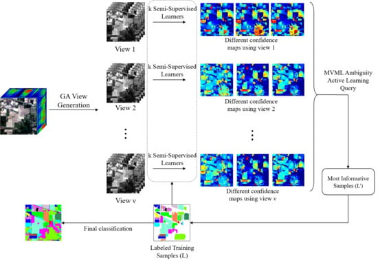
2.2. General Framework

This paper introduces an encapsulated framework designed to integrate spectral-spatial semi-supervised learning (SS-SSL) and MVML-AL, and to take advantage of both SSL and AL to incorporate unlabeled samples in different ways. In other words, we employed an SS-SSL method as the classifier and MVML-AL as a wrapper active learning method, which aims to enlarge the labeled training set intelligently. To generate different views, we adopted an automatic genetic algorithm feature subset selection (GA-FSS) method based on maximizing inter-views and intra-views confidences, which characterize dependency and sufficiency, respectively. Then, the probabilistic ambiguity measure was developed as the heuristic query function of MVML-AL. Figure 1 shows the flowchart of the proposed method in detail.

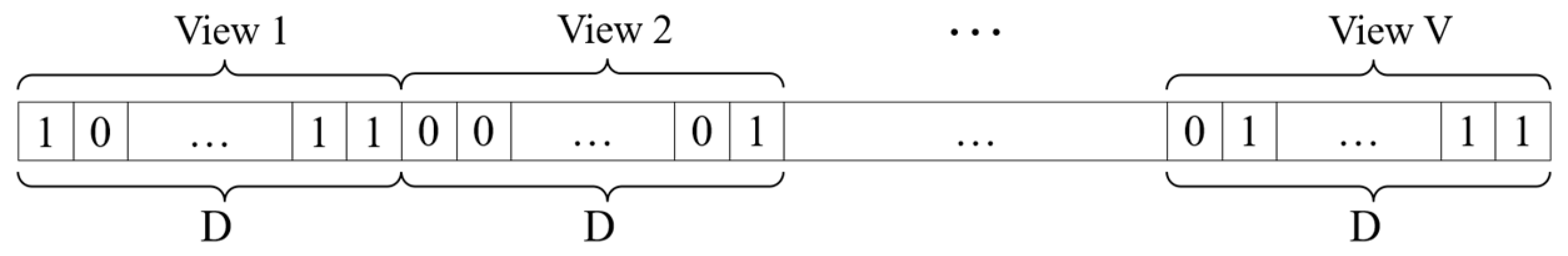
2.2.1. View Generation by GA-FSS

This stage aims to construct multiple diverse, sufficient, and as independent as possible views by employing a GA, which is one of the most famous evolutionary computation techniques for FSS [32,33,34]. Depending on whether the learning performance is used to contribute to the fitness function or not, the FSS methods are divided into two broad categories: (1) wrapper approaches and (2) filter approaches. In the proposed GA scheme, a binary chromosome is used with the size of V multiplied by D, where V is the number of views, and D represents the original feature dimension of the dataset. The first D bits denote the selected features of the first view, based on whether each band is selected or not, and the corresponding bit is 1 or 0. Figure 2 shows the chromosomal design in our proposed view generation method.

We used a hybrid approach using both filter (i.e., inter-view confidence) and wrapper (i.e., intra-view confidence) criteria to build the fitness function. A weighted summation combines these two evaluation measures with corresponding weights $w_f$ and $w_w$ for filter and wrapper, respectively. Therefore, the qualification of each chromosome of the GA population (ch) is assessed by the fitness function below.

$$Fi{t}_{\left(ch\right)}=w_f\ast Filte{r}_{\left(ch\right)}+w_w\ast Wrappe{r}_{\left(ch\right)}.$$

(1)

The weights are experimentally set to $w_f$ = $w_w$ = 0.5. The filter part of the above fitness function must be designed to ensure the maximum diversity of all distinct views. We employed the mutual information (MI) method [35] to measure the amount of independence between each different pair of views of the chromosome. Therefore, $I\left(X^i,X^j\right)$ is the MI between views i and j, where $X^i$ and $X^j$ are associated subsets of the original data set, X_N×D. N is the number of all pixels throughout the image, and D is the number of spectral bands of the image. Finally, inter-confidence criterion ($C_{inter}$) is defined as the filter part as follows:

$$Filte{r}_{\left(ch\right)}=C_{inter}\left(X\right)={\sum }_{i=1}^V{\sum }_{j=1}^V\frac{1}{I\left(X^i,X^j\right)}.$$

(2)

The view sufficiency is defined by the intra-confidence, which is the mean of the classifier performance on all views. The classifier performance on the view i is estimated by a function named P_i using the provided labeled training samples. X_L, X_U, and Y_L are the labeled samples, the unlabeled samples, and the labels provided for the training set, respectively. Consequently, $X_L^i$ and $X_U^i$, are the corresponding subsets of X_L and X_U, according to the view i. Therefore, the wrapper part of the GA fitness function that represents sufficiency is formed as follows.

$$Wrappe{r}_{\left(ch\right)}=C_{intra}\left(X\right)=\frac{1}{V}{\sum }_{i=1}^V{P}_i\left(X_L^i,X_U^i,Y_L\right).$$

(3)

To implement GA to generate an optimal subset of views, the initial population with 50 chromosomes was randomly generated. The other parameters of GA were chosen as follows: 5%, 20% and 80% as the rates of mutation, migration, and crossover; 200 as the maximum number of generations; and 20 as the maximum number of generations with no significant improvement in the fitness function, all which are common choices in similar GA optimization cases [34].

2.2.2. MVML Sampling Strategy

In our proposed method, the multiple learners at each view are adapted for a more accurate estimation of each samples’ information content. Although the entropy maximization is one of the previously used measures to compute disagreement level between learners [23], it cannot retain its different ability in the MVML framework. Therefore, the ambiguity measure was proposed in [21] and demonstrated outstanding performance. However, there is still room for improvement by incorporating the classifiers’ confidence. The original method counts merely the number of learners that agree to assign a specific label to the sample while disregarding each learner’s confidence that it has a significant influence on the selected samples. We proposed a probabilistic-ambiguity measure that contributes to the confidence level of each learner at each view and computes disagreement between all the views.

Suppose we construct V distinct views for a multi-class classification problem with Nc classes and k learners that are combined at each view. For each sample, the confidence that the view i assigns the sample to the class j, $P_j^i$ is computed as follows. k is the number of the learners combined at each view, and $p_{m,j}^i$ is the mth learner’s confidence considering the ith view to classifying the sample as class j.

$$P_j^i=\frac{r/2+{\sum }_{m=1}^k{p}_{m,j}^i}{r+k},$$

(4)

where r is a small positive constant, which is added to prevent zero value of the confidence. Then, the general confidence of each label is also calculated, which can be interpreted as the average prediction confidence of all the views.

$$P_j=\frac{r/2+{\sum }_{i=1}^V{\sum }_{m=1}^k{p}_{m,j}^i}{r+k}.$$

(5)

Although one can use an entropy measure of the calculated confidences of each class $P_j$, we adopted the ambiguity measure because of its better performance, which will be proven by the ensuing experimental results. In Equation (6), $c_i$ is the allocated label to the sample by the majority vote of all the learners at view i.

$$ambiguity\left(x\right)=C_x\left(-1-{\sum }_{i=1}^V{P}_{c_i}^i\log P_{c_i}^i\right).$$

(6)

In this definition, the variable $C_x$ indicates agreement or disagreement of the predicted labels considering their different views; hence, if $c_1=c_2=\cdots =c_V$, that means all the views predict the same label for the sample and completely agree with each other; then, $C_x=1$; otherwise, $C_x=-1$. In this way, $C_x$ plays an important role in the selection strategy, because it defines the behavior of the main ambiguity function; i.e., whether all views agree together about that sample or not. In this way, the samples with disagreement are ranked higher as the more informative samples.

2.2.3. Semi-Supervised Learning Algorithm

The primary goal of the proposed SSL algorithm is finding a real-valued labeling function $f:V\to \mathbb{R}$ on the graph G, and then assigning a label to each unlabeled sample. The f should be consistent with the initial labels of the labeled samples. Furthermore, the labeling function must be smooth over the graph G, which indicates that the samples that are close together must have a similar label, and the difference between predicted labels defines the cost function. L is the combinatorial Laplacian of the graph.

$$C\left(f\right)={\sum }_{i,j}{w}_{ij}{\left(f_i-f_j\right)}^2=2f^{T}Lf.$$

(7)

In other words, as the points are closer to each other, a severe change in the labeling function imposes a higher cost. Hence, the labeling function over the graph is provided by the optimization problem by considering the initial label samples ($X_L,Y_L$).

$$f=\arg \underset{f|X_L=Y_L}{\min }C\left(f\right).$$

(8)

To solve the above optimization problem (i.e., Equation (8)), we used harmonic cost minimization by considering the Gaussian random field [36]. In this paper, a spectral-spatial SSL algorithm was used as the base classification framework. First, two distinct spectral and spatial graphs were constructed, wherein each sample connected to it had k-nearest spectral and l-nearest spatial neighbors, respectively. In the spectral graph, each pixel in the image is connected to its k-nearest neighbors in the spectral space. The weight of the connecting edge is calculated based on the spectral similarity between the vertices [37]. The radial basis function (RBF) kernel of width σ calculates the similarity between data points:

$$w_{ij}=\exp (\frac{-\Vert x_i-x_j{\Vert }^2}{2{\sigma }^2})$$

(9)

To avoid self-similarity, $w_{ii}$ is set to zero. The spatial-based graph is constructed based on the spectral distance between each pixel and its spatial neighbors. In the conventional spatial graph, each pixel is connected to 4, 8, 12, 20, and 24 spatial neighbors, considering the size of the image. The laplacians of each graph ($L_{spect}$ and $L_{spat})$ are computed based on the weight of the existing edges; L = D − W, where W is the affinity matrix and D is the diagonal matrix defined by $D_{ii}={\sum }_j{w}_{ij}.$ Then, the graphs are combined by a weighted sum of their Laplacian matrices [38,39].

$$L_T=\gamma L_{spect}+\left(1-\gamma \right)L_{spat}$$

(10)

In this way, the weighted joint graph Laplacian (LT) is constructed and replaced in Equation (7). Then, semi-supervised learning uses a harmonic cost minimization approach to minimize the cost function on both spectral and spatial graphs simultaneously. Therefore, the labeling function for unlabeled samples is given as follows:

$$f_u=-L_{T_{uu}}^{-1}{L}_{T_{ul}}{f}_l,$$

(11)

where L_T should be partitioned into 2 × 2 blocks for labeled and unlabeled nods as $L_T=\left[\begin{array}{cc}{L}_{T_{ll}}& L_{T_{lu}}\\ L_{T_{ul}}& L_{T_{uu}}\end{array}\right]$. It can be demonstrated that for each sample $x_i$, ${\sum }_{j=1}^k{f}_{ij}=1$. Therefore, we can regard $f_{ij}$ as the probability of $x_i$ to the jth class $P\left(c^j|x_i\right)$. Each unlabeled sample is assigned to the class with the highest probability.

3. Results

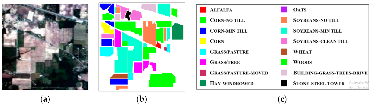
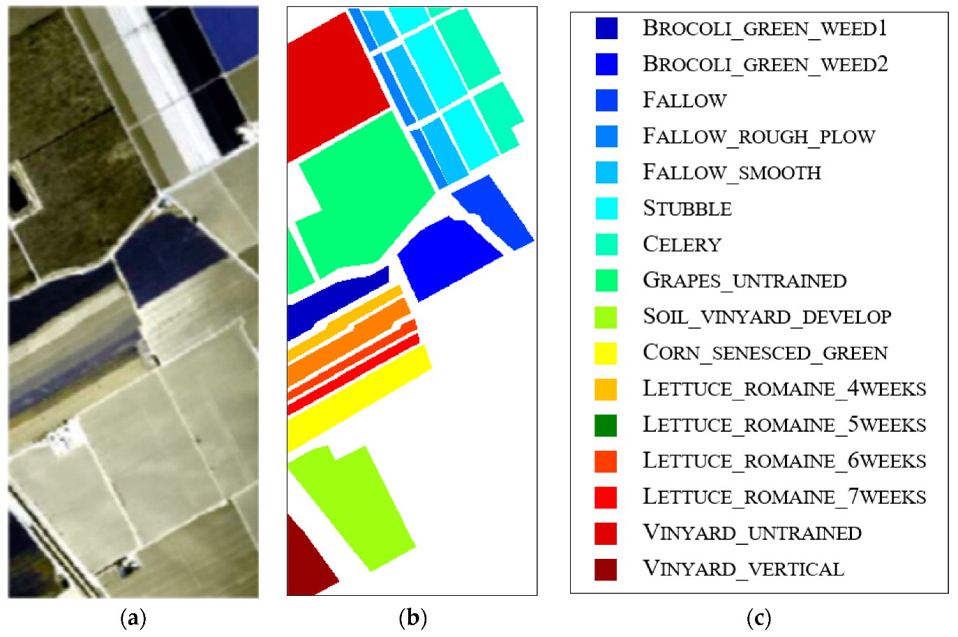
3.1. Hyperspectral Data

Our experiments, including the proposed method and the competitor methods, were conducted on three widely used hyperspectral data sets: Indian Pines, Salinas, and Pavia University. The Indian Pines and Salinas data sets were acquired by an airborne visible/infrared imaging spectrometer (AVIRIS) sensor, which initially provided 220 spectral images with different spatial resolutions of 20 m and 3.7 m in that order. An Indian Pines image with a size of 145 by 145 pixels is given in Figure 3a. The available ground truth (Figure 3b) contains 16 different agricultural land cover classes ranging in size from 20 to 2468 pixels per class.

The Salinas image was captured over Salinas Valley, California. The AVIRIS sensor measured 16 different classes from different agriculture crops. It has a precious ground truth containing more than 54,000 samples, which is an adequate number, and the smallest and largest classes have 916 and 11,271 samples, respectively. Figure 4a,b shows the true-color image of the dataset and the ground truth map.

The Pavia University data set was provided by a reflective optics system imaging spectrometer (ROSIS) 610 by 340 pixels in size. The spatial and spectral resolutions provided by the ROSIS sensor are 1.3 m and 115 bands, respectively. Pavia University is an urban area with nine different classes that are shown in Figure 5a,b.

3.2. Experimental Setup

The hyperspectral bands were normalized in the range from 0 to 1 to provide numerical stability in calculations and graph matrices. Tuning of the free parameters is one of the most sensitive and essential steps to obtaining an optimal classifier. The proposed SSL classifier has only two free parameters: the kernel width parameter (σ) and the weight of the spectral graph (γ). The best values are defined by a 2-D grid search method with a search space of 0.05, 0.1, 0.15, …, 0.95.

The experiment was conducted using a well-designed cross-validation scheme to test the model’s ability with separate training and test data sets. Two different “k-fold” and “hold-out” cross-validation methods were combined to generate a statistically unbiased classification problem, and a small labeled training set, since the AL algorithm was proposed to overcome difficulties of the inadequately labeled dataset. The worst-case scenario with the minimum number of labeled samples, i.e., only three pixels per class, was chosen as the initial state for a fair comparison between the proposed method and different conventional AL methods. At each step, the five most informative pixels were selected and added to the labeled training set. The maximum number of iterations was set to 40, which means the training set was enlarged by adding 200 samples at the end of each algorithm.

More precisely, the initial labeled samples were selected by three pixels per class; i.e., $\Vert L_0\Vert =48$ for Indian Pines and Salinas, and $\Vert L_0\Vert =27$ for Pavia University. At the final iteration, the labeled training set was enlarged by adding 200 samples, which means $\Vert L_{40}\Vert =248$, and $\Vert L_{40}\Vert =227$. The ground truth (GT) size of each data set is, respectively, 21,025, 207,400, and 111,104 samples. The final sizes of the training sets were only 1.17%, 0.11%, and 0.22% of the labeled GT samples. The average overall accuracy ($\overline{OA}$) and kappa index ($\overline{\mathrm{K}}$) over five-fold were reported as the evaluation metrics of the different baseline and proposed methods.

3.3. Experimental Results

For a comprehensive evaluation of the proposed MVML method, well-known algorithms of the other three main AL categories with the best performance were implemented and compared to the proposed method. Breaking tie (BT) [2] is one of the simplest and high-performance AL methods that was implemented here as the representative of the SVSL category. The GA-comb method was implemented from the MVSL category, which used our proposed view generation method with AMD AL query function [28]. The third comparative SVML method is mQBC-kernels [25]. It was also compared to another MVML method, named entropy to demonstrate the best performance of the proposed MVML-ambiguity method, [40].

The number of kernels and views for the proposed MVML-AL algorithm are selected using a 2D grid-search with the search space {2, 3, 4, 5, 6, 7} for the number of views and {2, 3, 4, 5} for the number of learners. Then the cost-performance trade-off is considered to find the optimal values of each parameter with the highest performance of the algorithm and the lowest computational cost. Therefore, the MVML methods were implemented by employing four different kernel type learners, including linear, polynomial, sigmoid, and RBF, which were used to compute the similarities between the connected samples in the graph. Also, there were two distinct views, which were generated by the proposed GA-Comb framework. Each experiment was conducted using five randomly selected initial training data sets, and the average overall accuracy ($\overline{\mathrm{OA}}$) in percentage was reported as the performance evaluation.

In remote sensing context, the accuracy of classification methods is usually evaluated by kappa coefficients. Therefore, the Z-value statistical test [41] will determine the significant difference of two kappa coefficients as follows. ${\widehat{k}}_1$ and ${\widehat{k}}_2$ are the mean value of the kappa coefficients derived from two different classification algorithms with different training sets, and ${\sigma }_{k_1}^2$ and ${\sigma }_{k_2}^2$ are the corresponding variances.

$$\left|Z\right|=\frac{{\widehat{k}}_1-{\widehat{k}}_2}{\sqrt{{\sigma }_{k_1}^2+{\sigma }_{k_2}^2}}.$$

(12)

Based on the test with the 5% significance level, the difference between the two algorithms are statistically significant if $\left|Z\right|>1.96$.

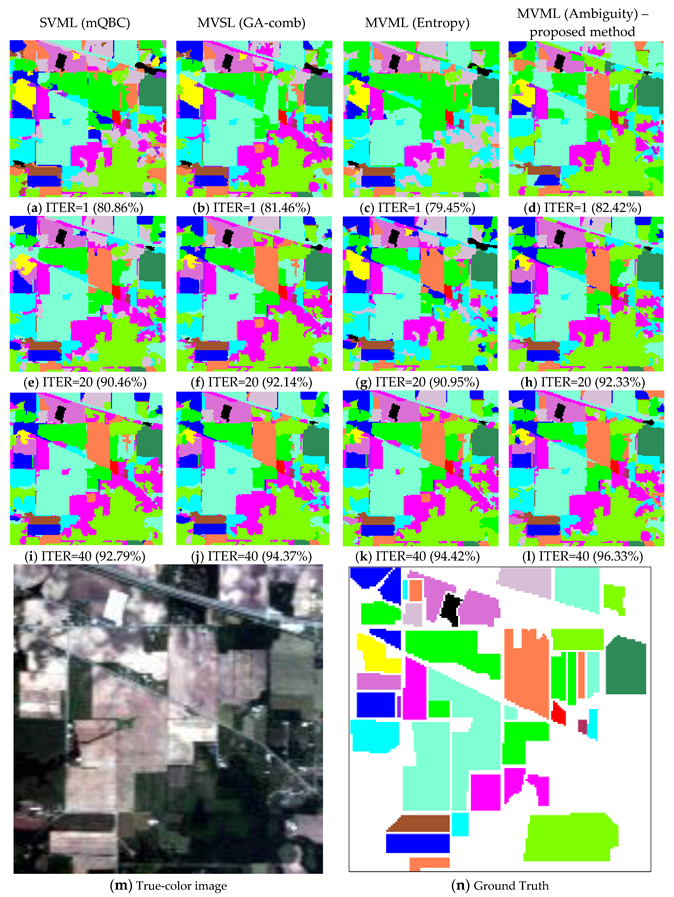
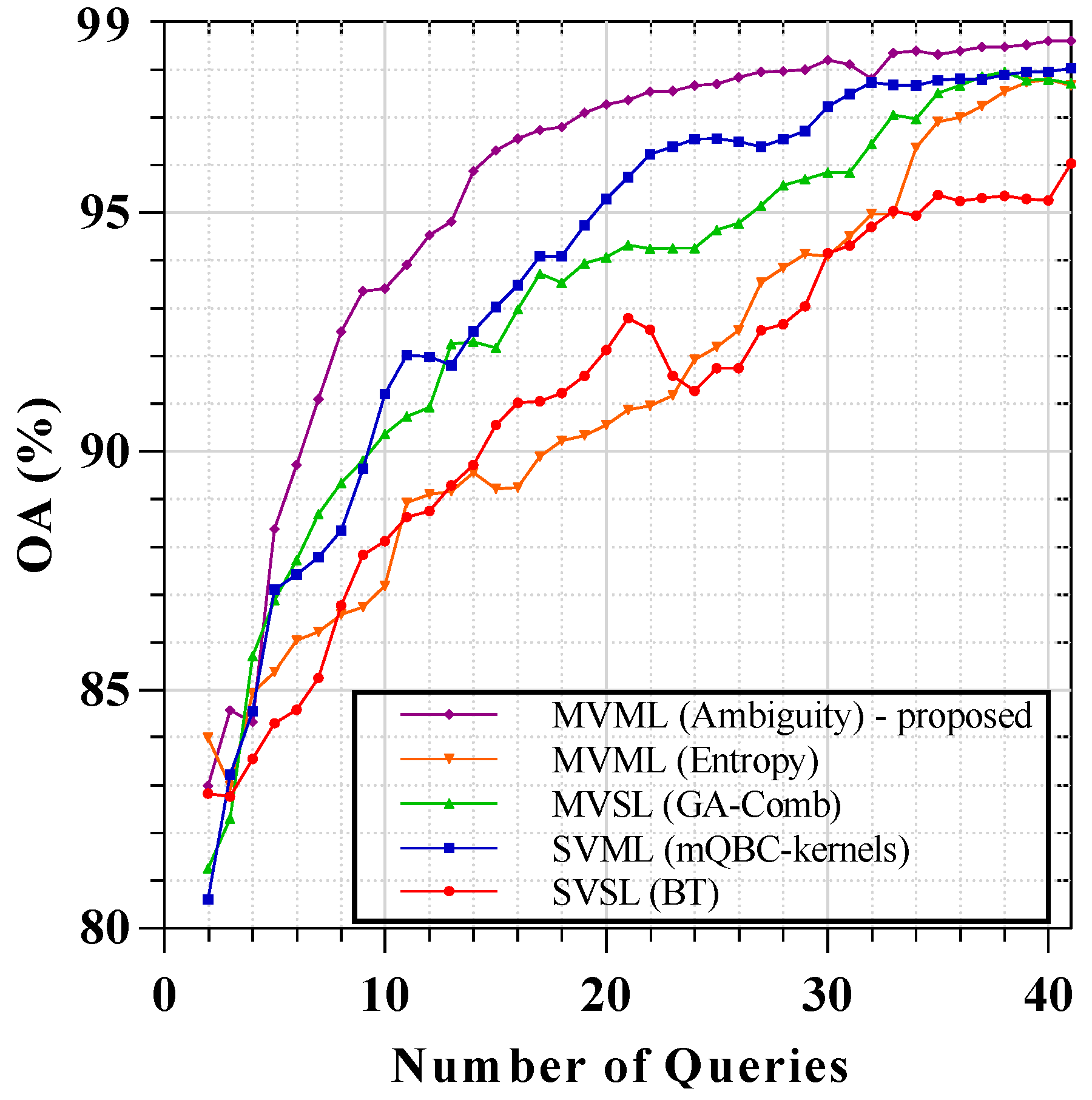
3.3.1. Results of AVIRIS Indian Pine Image

To demonstrate the superiority of the proposed MVML selection strategy, the best-performing methods of the other categories were included for comparison. Figure 6 presents the learning curve of different AL schemes for the Indian Pine data set.

Although the other traditional categories of active learning methods achieved excellent results, the MVML method, especially when using the proposed ambiguity query function, could improve the performance.

Table 1. Average overall accuracy ($\overline{\mathrm{OA}}$) achieved on the Indian pines dataset after 1, 10, 20, 30, and 40 iterations with a batch size of five samples. The average amounts of accuracy incremented over the ten prior iterations are given in the second column ($\overline{\mathrm{diff}}$). All the results were averaged over five runs, and the best results are presented in bold.

Methods	ITER = 1		ITER = 10		ITER = 20		ITER = 30		ITE = 40
	$\overline{\mathbf{OA}}$	$\overline{\mathbf{diff}}$	$\overline{\mathbf{OA}}$	$\overline{\mathbf{diff}}$	$\overline{\mathbf{OA}}$	$\overline{\mathbf{diff}}$	$\overline{\mathbf{OA}}$	$\overline{\mathbf{diff}}$	$\overline{\mathbf{OA}}$	$\overline{\mathbf{diff}}$
SVSL (BT)	76.74	0.8	83.44	0.68	87.44	0.36	90.20	0.35	91.10	0.04
SVML (mQBC-kernels)	80.36	1.06	86.49	0.62	90.58	0.39	92.57	0.18	93.07	0.08
MVSL (GA-Comb)	81.51	1.05	89.32	0.84	92.03	0.21	93.96	0.21	94.83	0.07
MVML (entropy)	78.29	0.18	87.99	0.83	90.74	0.28	93.80	0.28	95.39	0.17
MVML (ambiguity)	82.17	1.71	89.97	0.98	91.83	0.14	95.08	0.33	97.14	0.20

presents the numerical results of these different methods at iteration numbers 1, 10, 20, 30, and 40. The average overall accuracy (OA) presents the classification performances over the five runs of each algorithm by the different randomly selected initial training set. At the final iteration, BT achieved the lowest performance with an OA equal to 91.10%, which is ≈6% lower than the proposed method. As expected, SVML and MVSL methods showed a higher performance compared to BT. However, our proposed method can improve the final classification performance significantly in comparison with SVML ($\left|Z\right|=9.3704>1.96$), SVML ($\left|Z\right|=6.8599>1.96$), MVSL ($\left|Z\right|=5.1450>1.96$), and MVML-entropy ($\left|Z\right|=3.3400>1.96$). The Z-values were computed based on Equation (12). As shown in this table, except for the 20th iteration, the proposed methods achieved the best performance.

In addition, the accuracy increment averages over the ten past iterations are given in the second column as $\overline{\mathrm{diff}}$, which represents the mean slope of four equal parts of the presented accuracy curves. For the first iteration, this quantity shows the difference between the first iteration and the initial classification accuracy. Therefore, the proposed method improved the initial results at the first iteration (1.7%), more than other baseline methods. According to Table 1, the proposed method (MVML-ambiguity) has the largest slope and improvement at the first steps and converges to a higher achievement compared to the baseline methods. In addition, the classified maps of the proposed and compared methods at iteration numbers of 1, 20, and 40 are given in Figure 7a–l, respectively. Since we employed a sophisticated spectral-spatial GB-SSL classifier, the emerged maps originally had a satisfactory presentation with homogenous objects and accurate borders. However, the proposed ambiguity AL method improved the achieved accuracies and the classification performances in the largest amount at all the iterations.

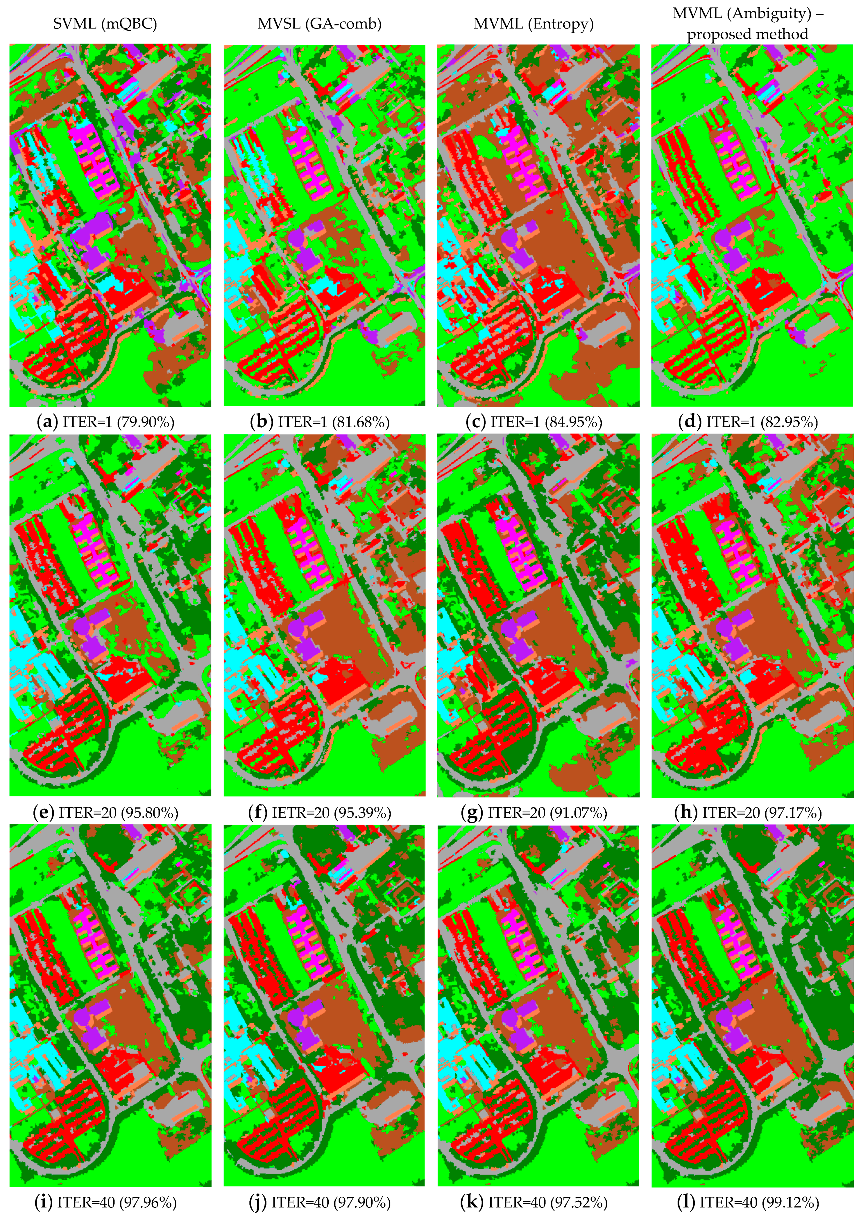
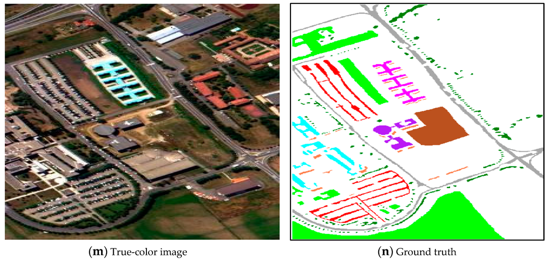
3.3.2. Results of ROSIS University of Pavia

Similar results for Pavia University data are given in Figure 8. In this data set, the observed improvement by the proposed MVML-ambiguity method is more significant, while the MVML-entropy method is more like the SVSL and MVSL methods.

The corresponding numerical results are presented in

Table 2. Average overall accuracy ($\overline{\mathrm{OA}}$) achieved on Pavia University dataset after 1, 10, 20, 30, and 40 iterations with a batch size of five samples. The average amounts of accuracy incremented over the ten prior iterations are given in the second column ($\overline{\mathrm{diff}}$). All the results were averaged over five runs, and the best results are presented in bold.

Methods	ITER = 1		ITER = 10		ITER = 20		ITER = 30		ITER = 40
	$\overline{\mathbf{OA}}$	$\overline{\mathbf{diff}}$	$\overline{\mathbf{OA}}$	$\overline{\mathbf{diff}}$	$\overline{\mathbf{OA}}$	$\overline{\mathbf{diff}}$	$\overline{\mathbf{OA}}$	$\overline{\mathbf{diff}}$	$\overline{\mathbf{OA}}$	$\overline{\mathbf{diff}}$
SVSL (BT)	82.81	0.44	88.62	0.59	92.78	0.38	94.31	0.21	96.02	0.14
SVML (mQBC-kernels)	80.60	0.33	92.01	1.15	95.75	0.42	97.48	0.15	98.03	0.03
MVSL (GA-Comb)	81.25	1.11	90.72	0.96	94.32	0.33	95.84	0.22	97.70	0.13
MVML (Entropy)	84.00	0.29	88.92	0.50	90.87	0.18	94.49	0.40	97.66	0.30
MVML (Ambiguity)	82.99	2.77	93.90	1.13	97.36	0.30	98.10	0.02	98.59	0.08

, which shows that the proposed method made the most significant improvement at the first step (2.7%), which led to a stable superiority of this method throughout almost all iterations. Although in this data set, the final performance of the proposed method was closer to the comparative methods, it achieved the highest performance (98.95%). The proposed method achieved 2.57% higher OA ($\left|Z\right|=4.4075>1.96$) at the final iteration in comparison with the SVSL method. According to Table 2, the MVSL is the nearest method in terms of numerical results to the proposed method. However, the difference between them was still statistically significant ($\left|Z\right|=3.1466>1.96$).

In addition, Figure 9a–l represents the corresponding classified maps at the first, middle, and final iterations for the different AL methods, namely, SVML (mQBC), MVSL (GA-comb), MVML (entropy), and MVML (ambiguity). Since the Pavia university data set was acquired with a higher spatial resolution, the improvements of the proposed AL method improved the final land-cover classification maps more significantly. Also, the reported numerical results in Table 2 confirm the superiority of the proposed MVML-AL method.

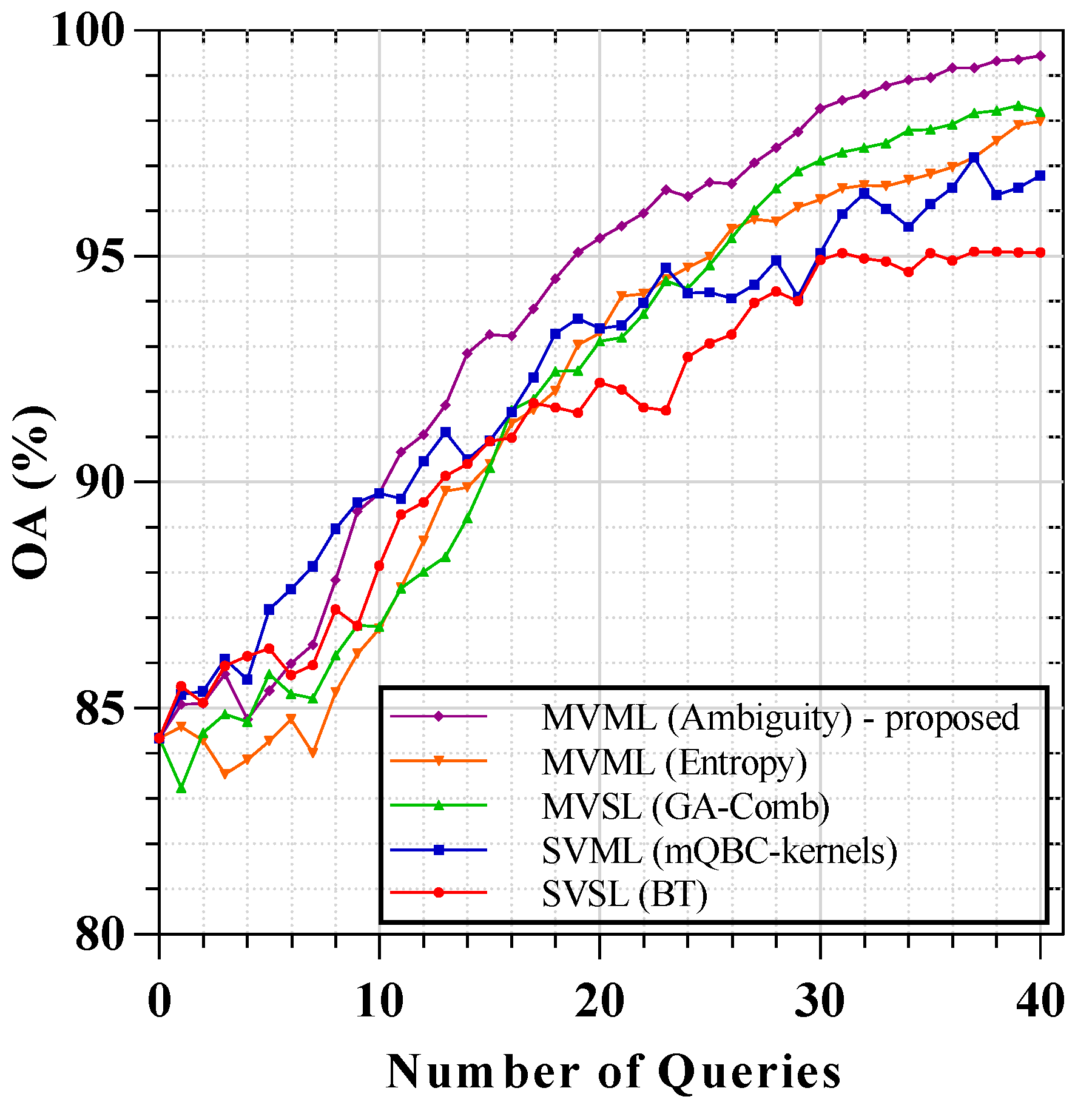
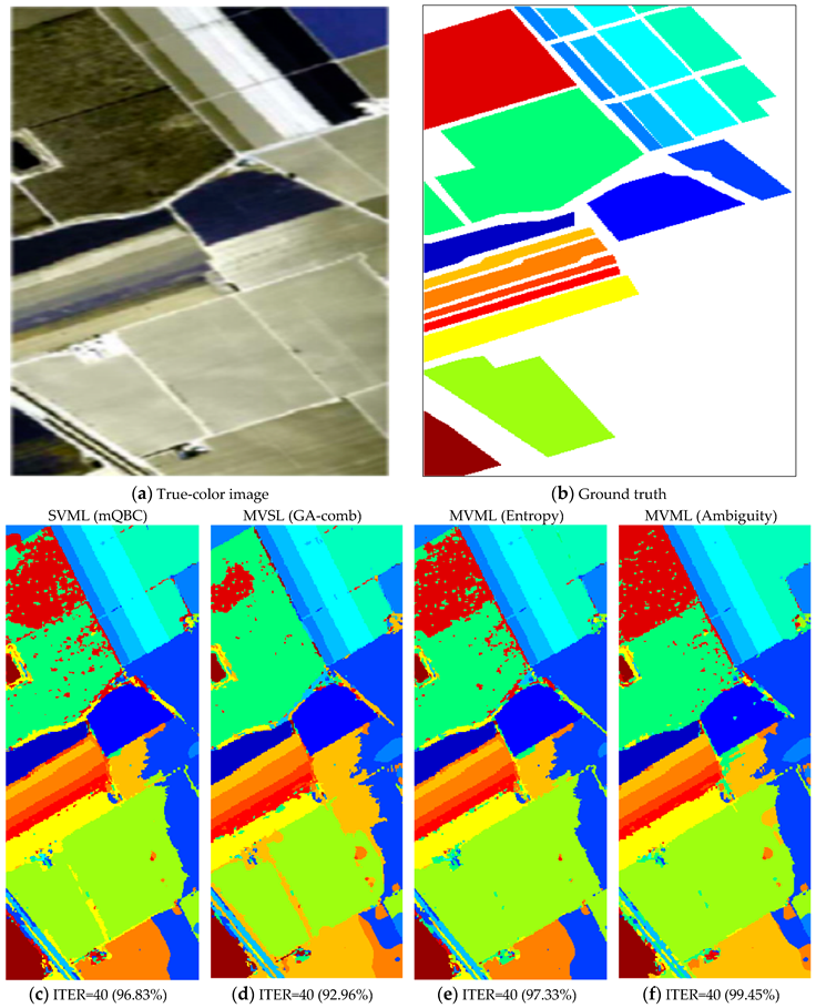
3.3.3. Results of AVIRIS Salinas Valley

Figure 10 and

Table 3. Average overall accuracy ($\overline{\mathrm{OA}}$) achieved on Salinas dataset after 1, 10, 20, 30, and 40 iterations with a batch size of five samples. The average amounts of accuracy incremented over the ten prior iterations are given in the second column ($\overline{\mathrm{diff}}$). All the results were averaged over five runs, and the best results are presented in bold.

Methods	ITER = 1		ITER = 10		ITER = 20		ITER = 30		ITER = 40
	$\overline{\mathbf{OA}}$	$\overline{\mathbf{diff}}$	$\overline{\mathbf{OA}}$	$\overline{\mathbf{diff}}$	$\overline{\mathbf{OA}}$	$\overline{\mathbf{diff}}$	$\overline{\mathbf{OA}}$	$\overline{\mathbf{diff}}$	$\overline{\mathbf{OA}}$	$\overline{\mathbf{diff}}$
SVSL (BT)	85.49	1.14	88.15	0.38	92.21	0.27	94.92	0.30	95.08	0.00
SVML (mQBC-kernels)	85.31	0.96	89.76	0.43	93.40	0.38	95.07	0.24	96.79	0.09
MVSL (GA-Comb)	83.24	−1.10	86.80	0.44	93.12	0.55	97.13	0.40	98.21	0.10
MVML (Entropy)	84.60	0.25	86.75	0.30	93.31	0.64	96.26	0.23	97.99	0.16
MVML (Ambiguity)	85.10	0.75	89.95	0.55	95.41	0.50	98.27	0.27	99.45	0.11

illustrate the overall accuracy curves and the average overall accuracies of the proposed and compared methods for the Salinas Valley data set, respectively.

Although after the first ten iterations, the proposed method was very close to the other methods, from that point on, it made a significant difference and achieved the best improvement. After 40 iterations, and by adding 200 new labeled samples to the training set, the proposed method achieved an outstanding performance of 99.45%, which was significantly higher than the baseline ones. The final classified maps by the various AL schemes are presented in Figure 11c–f. By comparing Figure 11f with other maps, it is obvious that the emerged classes were more homogenous and isolated pixels were reduced.

4. Discussion

4.1. Statistical Significance Analysis

As has been presented, the proposed method performed outstandingly in the conducted experimental results. However, to prove the effectiveness of the method, we made a new comparison with a number of recent state-of-the-art methods. Since our method took advantage of both SSL and AL methods, only AL-SSL methods were added to be compared. The compared methods include collaborative active and semi-supervised learning (CASSL) [42], random walker-based AL and SSL framework (RWASL) [14], Markov random field model-based active learning (MRF-AL) [43], and MVML-AL [21]. The final results of each method and the statistical significance of the proposed method, in comparison with them, are reported in

Table 4. Performance comparison between four compared methods (CASSL, RWASL, MRF-AL, and MVML-AL) and the modified MVML-AL. Average kappa index values and standard deviations ($\mathrm{s}$) obtained over five different training sets for all considered hyperspectral datasets. The reported Z-scores ($\left|\mathrm{Z}\right|$) indicate the significance, respectively, of the difference between each algorithm and the proposed one.

Methods	Indian Pines			Pavia University			Salinas
	$\mathbf{kappa}$	$\mathbf{s}$	$\left|\mathbf{Z}\right|$	$\mathbf{kappa}$	$\mathbf{s}$	$\left|\mathbf{Z}\right|$	$\mathbf{kappa}$	$\mathbf{s}$	$\left|\mathbf{Z}\right|$
CASSL [42]	0.939	0.0058	4.189	0.955	0.0025	7.208	0.982	0.0034	3.078
RWASL [14]	0.976	0.0056	−0.970	0.982	0.0046	0.524	0.991	0.0025	0.732
MRF-AL [43]	0.891	0.0150	5.007	0.911	0.0191	3.814	0.974	0.0087	2.166
MVML-AL [21]	0.953	0.0062	2.136	0.946	0.0036	7.786	0.987	0.0049	1.194
MVML-AL-proposed	0.969	0.0042	----	0.985	0.0034	----	0.993	0.0011	----

.

Although all of these algorithms performed well, our method achieved the best numerical classification accuracy after 40 iterations almost over all three datasets. Only in the Indian Pines dataset did the RWSAL algorithm show the best performance ($\mathrm{KAPPA}=0.976$), rather than the proposed modified-MVML-AL method ($\mathrm{KAPPA}=0.969$). However, the differences between these two methods were not significant ($\left|Z\right|=-0.970<1.96$) for Indian Pines, ($\left|Z\right|=-0.524<1.96$), the Pavia University, and ($\left|Z\right|=0.732>1.96$) for the Salinas datasets, respectively, which means that their performances were very close.

4.2. Different View Generation Methods

The different basic view generation methods [18], such as uniform, correlation, and k-means, were employed as the compared methods, and the selection strategy was AMD [18] for all methods. In this experiment, the number of views was chosen as two (distinct views), which led to satisfactory results and low computational cost simultaneously. As expected, the proposed view generation method using GAs (GA-comb) had the best performance, while the other three baseline view generation methods had similar results to some extent.

4.2.1. Views’ Diversity Analysis

To summarize, our novel GA-based view generation method has simultaneously maximized the diversity and efficiency of the views. To demonstrate our method’s better performance, we investigated the amount of mutual information as a measure of view dependency. The higher value of mutual information indicates that views have more correlation and dependency on each other. We aimed to produce more independent views that maximize diversity to construct more diverse classifiers. The amount of mutual information between two views for different data sets is reported in

Table 5. Mutual Information (MI) and average overall accuracy ($\overline{\mathrm{OA}}$) of the views by different view generation methods. The average accuracy was computed using 5-fold cross-validation.

Methods	Indian Pines			Pavia University			Salinas
	MI	$\overline{\mathbf{OA}}(\%)$		MI	$\overline{\mathbf{OA}}(\%)$		MI	$\overline{\mathbf{OA}}(\%)$
		View1	View2		View1	View2		View1	View2
Uniform	3.25	77.54	0.7653	3.08	82.13	81.96	4.76	84.63	85.07
Correlation	5.21	76.59	77.36	3.79	81.02	81.82	5.09	84.73	84.85
K-Means	4.25	77.96	78.01	3.52	82.09	82.10	4.97	84.36	83.97
Random	5.26	75.89	76.34	3.68	82.09	82.18	4.82	84.23	84.36
GA-filter	1.36	77.63	77.54	1.13	82.16	81.86	1.27	84.75	84.37
GA-Wrapper	2.56	78.47	78.94	3.22	84.09	83.68	4.37	85.94	86.21
GA-Comb	1.78	79.37	78.51	1.20	83.97	83.62	1.11	85.47	85.75

.

We investigated three different GA-based view generation methods: filter, wrapper, and a combinatorial method that used both criteria to provide more diverse and efficient views. As shown, the proposed GA-based methods significantly reduced the mutual information and dependency between views, which were 1.78, 1.20, and 1.11 for three data sets. The MIs achieved by the proposed method were much lower than the conventional methods. For instance, the uniform view generation method showed the best performance of diversity with MI = 3.25 for Indian Pines, MI = 3.08 for Pavia University, and MI = 4.76 for the Salinas data set. Although the GA-filter method produced views with the minimum amount of mutual information, this method did not consider the efficiency of views, whereas the GA-comb method achieved satisfactory mutual information and more efficient views.

4.2.2. Views’ Efficiency Analysis

Multi-view learning methods aim to construct separate but also sufficient views that can accurately learn a classifier with each one. Although many view generation methods have been proposed so far, few of them consider the sufficiency of each view. In our proposed GA-based method, both efficiency and diversity were considered as the feature selection criteria. Therefore, the average classification performance at each view, with five different initial training sets, were considered as the efficiency measure. The comparison results of the different methods are given in Table 5. As expected, GA-wrapper and GA-comb methods achieved higher accuracies at the first iteration, and consequently, that led to higher performances in the AL accuracy curve for them. According to Table 5, the reported $\overline{\mathrm{OA}}$ indicates the sufficiency of each view. As shown, the wrapper GA-based view generation method constructs the sufficient views at the first iteration of AL for the classification purpose. The two distinct views generated by the GA-wrapper achieved 78.47–78.94%, 84.09–83.68%, and 85.94–86.21% of the average OA for Indian pines, Pavia University, and Salinas data sets, respectively. Although the GA-wrapper method constructs the more efficient views, GA-Comb method could build a set of views that were efficient and simultaneously diverse.

4.2.3. Time Complexity Analysis

To evaluate the computation complexity of the proposed method, the CPU time was measured at each iteration, and the average amount is presented in Figure 12.

All the algorithms were implemented using MATLAB software and on a computer with an Intel Core i7 2.5 GHz CPU with 12 GB RAM. Since at each iteration, the classification algorithm was run at least once, the required running time for a classification algorithm also was included as a benchmark. As shown in the graph, the SVSL methods are the fastest, which is the consequence of their simplicity. On the other hand, the MVML methods with the most substantial number of classifying models were the most time-consuming. Although in these MVML methods, the eight different models were used, by employing four learners from two views, the times were less than eight times that of SVSL method. Thus, although the proposed methods imposed greater computational complexity, which was expected, they were still executable and feasible by taking advantage of MATLAB’s parallel computing functions.

5. Conclusions

In this paper, we proposed a multi-view, multi-learner (MVML) active learning method to improve the learning curve by integrating the previously introduced multi-view and multi learner ALs. Consequently, the performance of the AL method improved at almost all iterations. Particularly in the first steps, when the initial labeled training samples were insufficient, this improvement was more significant and efficient. In almost all data sets, the slope of the learning curve of the proposed method at the beginning iterations was higher than those of the baseline methods. To the best of our knowledge, the MVML methods have not yet been adopted for remote sensing image classification, and this work is the first attempt to use the high potential of these methods for hyperspectral, active learning. Also in this paper, we proposed a new hybrid GA-based band selection method to generate the views that are as diverse as possible, and each one is efficient individually. The experimental results clearly demonstrated the efficiency and the superiority of the suggested GA-based MVML active learning method. Furthermore, the achieved improvement by the proposed algorithm was statistically significant compared to the other state-of-the-art AL methods. The only concern is the high computational complexity of this approach, which can be alleviated by the available parallel computing facilities.

References

1. Persello, C.; Bruzzone, L. Active and semisupervised learning for the classification of remote sensing images. Geoscience and Remote Sensing. IEEE Trans. Geosci. Remote Sens. 2014, 52, 6937–6956. [Google Scholar] [CrossRef]
2. Tuia, D.; Pasolli, E.; Emery, W. Using active learning to adapt remote sensing image classifiers. Remote Sens. Environ. 2011, 115, 2232–2242. [Google Scholar] [CrossRef]
3. Settles, B. Active Learning Literature Survey; University of Wisconsin: Madison, WI, USA, 2010; Volume 52, p. 11. [Google Scholar]
4. Reitmaier, T.; Sick, B. Let us know your decision: Pool-based active training of a generative classifier with the selection strategy 4DS. Inf. Sci. 2013, 230, 106–131. [Google Scholar] [CrossRef]
5. Crawford, M.M.; Tuia, D.; Yang, H.L. Active learning: Any value for classification of remotely sensed data? Proc. IEEE 2013, 101, 593–608. [Google Scholar] [CrossRef] [Green Version]
6. Hu, R.; Namee, B.M.; Delany, S.J. Off to a good start: Using clustering to select the initial training set in active learning. In Proceedings of the Twenty-Third International Florida Artificial Intelligence Research Society Conference (FLAIRS 2010), Menlo Park, CA, USA, 19–21 May 2010. [Google Scholar]
7. Yuan, W.; Han, Y.; Guan, D.; Lee, S.; Lee, Y.K. Initial training data selection for active learning. In Proceedings of the 5th International Conference on Ubiquitous Information Management and Communication, New York, NY, USA, 21–23 February 2011; p. 5. [Google Scholar]
8. Alajlan, N.; Pasolli, E.; Melgani, F.; Franzoso, A. Large-Scale Image Classification Using Active Learning. IEEE Geosci. Remote Sens. Lett. 2014, 11, 259–263. [Google Scholar] [CrossRef]
9. Guo, J.; Zhou, X.; Li, J.; Plaza, A.; Prasad, S. Superpixel-Based Active Learning and Online Feature Importance Learning for Hyperspectral Image Analysis. IEEE J. Sel. Top. Appl. Earth Obs. Remote Sens. 2017, 10, 347–359. [Google Scholar] [CrossRef]
10. Zhang, Z.; Pasolli, E.; Crawford, M.M.; Tilton, J.C. An Active Learning Framework for Hyperspectral Image Classification Using Hierarchical Segmentation. IEEE J. Sel. Top. Appl. Earth Obs. Remote Sens. 2016, 9, 640–654. [Google Scholar] [CrossRef]
11. Samat, A.; Li, J.; Liu, S.; Du, P.; Miao, Z.; Luo, J. Improved hyperspectral image classification by active learning using pre-designed mixed pixels. Pattern Recognit. 2016, 51, 43–58. [Google Scholar] [CrossRef]
12. Dopido, I.; Li, J.; Marpu, P.R.; Plaza, A.; Bioucas-Dias, J.M.; Benediktsson, J.A. Semi-supervised self-learning for hyperspectral image classification. IEEE Trans. Geosci. Remote Sens 2013, 51, 4032–4044. [Google Scholar] [CrossRef] [Green Version]
13. Tan, K.; Hu, J.; Li, J.; Du, P. A novel semi-supervised hyperspectral image classification approach based on spatial neighborhood information and classifier combination. ISPRS J. Photogramm. Remote Sens. 2015, 105, 19–29. [Google Scholar] [CrossRef]
14. Sun, B.; Kang, X.; Li, S.; Benediktsson, J.A. Random-Walker-Based Collaborative Learning for Hyperspectral Image Classification. IEEE Trans. Geosci. Remote Sens. 2017, 55, 212–222. [Google Scholar] [CrossRef]
15. Paoletti, M.; Haut, J.; Plaza, J.; Plaza, A. Deep learning classifiers for hyperspectral imaging: A review. ISPRS J. Photogramm. Remote Sens. 2019, 158, 279–317. [Google Scholar] [CrossRef]
16. Lin, J.; Zhao, L.; Li, S.; Ward, R.; Wang, Z.J. Active-Learning-Incorporated Deep Transfer Learning for Hyperspectral Image Classification. IEEE J. Sel. Top. Appl. Earth Obs. Remote Sens. 2018, 11, 4048–4062. [Google Scholar] [CrossRef]
17. Liu, P.; Zhang, H.; Eom, K.B. Active deep learning for classification of hyperspectral images. IEEE J. Sel. Top. Appl. Earth Obs. Remote Sens. 2016, 10, 712–724. [Google Scholar] [CrossRef] [Green Version]
18. Di, W.; Crawford, M.M. View generation for multiview maximum disagreement based active learning for hyperspectral image classification. Geosci. Remote Sens. IEEE Trans. 2012, 50, 1942–1954. [Google Scholar] [CrossRef]
19. Ma, L.; Ma, A.; Ju, C.; Li, X. Graph-based semi-supervised learning for spectral-spatial hyperspectral image classification. Pattern Recognit. Lett. 2016, 83, 133–142. [Google Scholar] [CrossRef]
20. Chen, Z.; Wang, B.; Niu, Y.; Xia, W.; Zhang, J.Q.; Hu, B. Semisupervised hyperspectral image classification based on affinity scoring. In Proceedings of the 2015 IEEE International Geoscience and Remote Sensing Symposium (IGARSS), Milan, Italy, 26–31 July 2015; pp. 4967–4970. [Google Scholar]
21. Zhang, Q.; Sun, S. Multiple-view multiple-learner active learning. Pattern Recognit. 2010, 43, 3113–3119. [Google Scholar] [CrossRef]
22. Freund, Y.; Seung, H.S.; Shamir, E.; Tishby, N. Selective sampling using the query by committee algorithm. Mach. Learn. 1997, 28, 133–168. [Google Scholar] [CrossRef]
23. Tuia, D.; Volpi, M.; Copa, L.; Kanevski, M.; Munoz-Mari, J. A survey of active learning algorithms for supervised remote sensing image classification. Sel. Top. Signal Process. IEEE J. 2010, 5, 606–617. [Google Scholar] [CrossRef]
24. Mamitsuka, N.A.H. Query learning strategies using boosting and bagging. In Machine Learning: Proceedings of the Fifteenth International Conference (ICML’98); Morgan Kaufmann Publishers: Burlington, MA, USA, 1998. [Google Scholar]
25. Zhou, Z.-H.; Li, M. Tri-training: Exploiting unlabeled data using three classifiers. IEEE Trans. Knowl. Data Eng. 2005, 17, 1529–1541. [Google Scholar] [CrossRef] [Green Version]
26. Wang, W.; Zhou, Z.H. Analyzing co-training style algorithms. In European Conference on Machine Learning; Springer: Berlin, Germany, 2007; pp. 454–465. [Google Scholar]
27. Xia, T.; Tao, D.; Mei, T.; Zhang, Y. Multiview spectral embedding. IEEE Trans. Syst. Man Cybern. Part B 2010, 40, 1438–1446. [Google Scholar]
28. Di, W.; Crawford, M.M. Active learning via multi-view and local proximity co-regularization for hyperspectral image classification. Sel. Top. Signal Process. IEEE J. 2011, 5, 618–628. [Google Scholar] [CrossRef] [Green Version]
29. Xu, C.; Tao, D.; Xu, C. A survey on multi-view learning. arXiv 2013, arXiv:1304.5634. [Google Scholar]
30. Sun, S.; Jin, F.; Tu, W. View construction for multi-view semi-supervised learning. Adv. Neural Netw. ISNN 2011, 2011, 595–601. [Google Scholar]
31. Muslea, I.; Minton, S.; Knoblock, C.A. Active+ semi-supervised learning= robust multi-view learning. In Proceedings of the ICML, Sydney, Australia, 8–12 July 2002; pp. 435–442. [Google Scholar]
32. Xue, B.; Zhang, M.; Browne, W.N.; Yao, X. A survey on evolutionary computation approaches to feature selection. IEEE Trans. Evol. Comput. 2016, 20, 606–626. [Google Scholar] [CrossRef] [Green Version]
33. Ghareb, A.S.; Bakar, A.A.; Hamdan, A.R. Hybrid feature selection based on enhanced genetic algorithm for text categorization. Expert Syst. Appl. 2016, 49, 31–47. [Google Scholar] [CrossRef]
34. Li, S.; Wu, H.; Wan, D.; Zhu, J. An effective feature selection method for hyperspectral image classification based on genetic algorithm and support vector machine. Knowl. Based Syst. 2011, 24, 40–48. [Google Scholar] [CrossRef]
35. Bennasar, M.; Hicks, Y.; Setchi, R. Feature selection using Joint Mutual Information Maximisation. Expert Syst. Appl. 2015, 42, 8520–8532. [Google Scholar] [CrossRef] [Green Version]
36. Zhu, X.; Ghahramani, Z.; Lafferty, J.D. Semi-supervised learning using gaussian fields and harmonic functions. In Proceedings of the 20th International Conference on Machine Learning (ICML-03), Washington, DC, USA, 21–24 August 2003; pp. 912–919. [Google Scholar]
37. Camps-Valls, G.; Bandos Marsheva, T.; Zhou, D. Semi-supervised graph-based hyperspectral image classification. Geosci. Remote Sens. IEEE Trans. 2007, 45, 3044–3054. [Google Scholar] [CrossRef]
38. Jamshidpour, N.; Safari, A.; Homayouni, S. Spectral–Spatial Semisupervised Hyperspectral Classification Using Adaptive Neighborhood. IEEE J. Sel. Top. Appl. Earth Obs. Remote Sens. 2017, 10, 4183–4197. [Google Scholar] [CrossRef]
39. Jamshidpour, N.; Homayouni, S.; Safari, A. Graph-based semi-supervised hyperspectral image classification using spatial information. In Proceedings of the 2016 8th Workshop on Hyperspectral Image and Signal Processing: Evolution in Remote Sensing (WHISPERS), Los Angeles, CA, USA, 21–24 August 2016; pp. 1–4. [Google Scholar]
40. Zhu, X.; Lafferty, J.; Ghahramani, Z. Combining active learning and semi-supervised learning using gaussian fields and harmonic functions. In Proceedings of the ICML 2003 Workshop on the Continuum from Labeled to Unlabeled Data in Machine Learning and Data Mining, Washington, DC, USA, 21 August 2003. [Google Scholar]
41. Foody, G.M. Classification accuracy comparison: Hypothesis tests and the use of confidence intervals in evaluations of difference, equivalence and non-inferiority. Remote Sens. Environ. 2009, 113, 1658–1663. [Google Scholar] [CrossRef] [Green Version]
42. Wan, L.; Tang, K.; Li, M.; Zhong, Y.; Qin, A. Collaborative active and semisupervised learning for hyperspectral remote sensing image classification. IEEE Trans. Geosci. Remote Sens. 2015, 53, 2384–2396. [Google Scholar] [CrossRef]
43. Sun, S.; Zhong, P.; Xiao, H.; Wang, R. An MRF model-based active learning framework for the spectral-spatial classification of hyperspectral imagery. IEEE J. Sel. Top. Signal Process. 2015, 9, 1074–1088. [Google Scholar] [CrossRef]
Figure 1. The proposed GA-MVML active learning method.
Remotesensing 12 00297 g001
Figure 2. The chromosomal design for the GA-FSS view generation scheme.
Remotesensing 12 00297 g002
Figure 3. The 145 × 145 AVIRIS Indian Pine data set. (a) True color composite with bands R:26, G:14, B:8. (b) Ground truth reference map. (c) Legend of the reference map with 16 land cover classes.
Remotesensing 12 00297 g003
Figure 4. The 512 × 217 AVIRIS Salinas Valley data set. (a) True color composite with bands R:26, G:14, B:8. (b) Ground truth reference map. (c) Legend of the reference map with 16 land cover classes.
Remotesensing 12 00297 g004
Figure 5. The 610 × 340 ROSIS Pavia University data set. (a) True color composite with bands R:53, G:31, B:8. (b) Ground truth reference map. (c) Legend of the reference map with nine land cover classes.
Remotesensing 12 00297 g005
Figure 6. Comparison of different categories of active learning methods for the Indian Pine data set.
Remotesensing 12 00297 g006
Figure 7. Classification maps of AVIRIS Indian Pines image. Each column represents the different AL method, and each row shows the different iteration of the algorithm. The overall accuracies in percent are reported below the maps.
Remotesensing 12 00297 g007
Figure 8. Comparison of different categories of active learning methods for Pavia University data set.
Remotesensing 12 00297 g008
Figure 9. Classification maps of Pavia University image. Each column represents the different AL method, and each row shows the different iterations of the algorithm. The overall accuracies in percent are reported below the maps.
Remotesensing 12 00297 g009aRemotesensing 12 00297 g009b
Figure 10. Comparison of different categories of active learning methods for the Salinas Valley data set.
Remotesensing 12 00297 g010
Figure 11. Classification maps of the final iteration of the algorithm for AVIRIS Salinas Valley image. Each column from c–f represents the different AL methods, namely, SVML (mQBC), MVSL (GA-comb), MVML (entropy), and MVML (ambiguity). The right map was produced by the proposed method. The overall accuracies in percent are reported above the maps.
Remotesensing 12 00297 g011
Figure 12. The average CPU times of different AL methods for a single iteration.
Remotesensing 12 00297 g012