Article

Investigation of Tightly Combined Single-Frequency and Single-Epoch Precise Positioning Using Multi-GNSS Data

1
GNSS Research Center, Wuhan University, 129 Luoyu Road, Wuhan 430000, China
2
Collaborative Innovation Center of Geospatial Technology, 129 Luoyu Road, Wuhan 430000, China
3
Qianxun Spatial Intelligence Inc., Bay Valley Hi-tech Park, North Guoquan Road, Shanghai 200000, China
*
Author to whom correspondence should be addressed.
Remote Sens. 2020, 12(2), 285; https://doi.org/10.3390/rs12020285
Submission received: 10 December 2019 / Revised: 7 January 2020 / Accepted: 13 January 2020 / Published: 15 January 2020

Abstract

:
The loose combination (LC) and the tight combination (TC) are two different models in the combined processing of four global navigation satellite systems (GNSSs). The former is easy to implement but may be unusable with few satellites, while the latter should cope with the inter-system bias (ISB) and is applicable for few tracked satellites. Furthermore, in both models, the inter-frequency bias (IFB) in the GLObal NAvigation Satellite System (GLONASS) system should also be removed. In this study, we aimed to investigate the performance difference of ambiguity resolution and position estimation between these two models simultaneously using the single-frequency data of all four systems (GPS + GLONASS + Galileo + BeiDou Navigation Satellite System (BDS)) in three different environments, i.e., in an open area, with surrounding high buildings, and under a block of high buildings. For this purpose, we first provide the definition of ISB and IFB from the perspective of the hardware delays, and then propose practical algorithms to estimate the IFB rate and ISB. Thereafter, a comprehensive performance comparison was made between the TC and LC models. Experiments were conducted to simulate the above three observation environments: the typical situation and situations suffering from signal obstruction with high elevation angles and limited azimuths, respectively. The results show that in a typical situation, the TC and LC models achieve a similar performance. However, when the satellite signals are severely obstructed and few satellites are tracked, the float solution and ambiguity fixing rates in the LC model are dramatically decreased, while in the TC model, there are only minor declines and the difference in the ambiguity fixing rates can be as large as 30%. The correctly fixed ambiguity rates in the TC model also had an improvement of around 10%. Once the ambiguity was fixed, both models achieved a similar positioning accuracy.

Graphical Abstract

1. Introduction

The Global Navigation Satellite System (GNSS) has entered into a new era in recent decades with four different systems operating simultaneously, i.e., American Global Positioning System (GPS), Russian GLObal NAvigation Satellite System (GLONASS), European Galileo, and Chinese BeiDou Navigation Satellite System (BDS), forming a joint multi-GNSS system. The increasing number of visible satellites have been confirmed to improve the satellite availability, convergence time, and reliability [1,2], and will bring great benefits to urban navigation services. Since satellite signals may be obstructed by the surrounding huge buildings or a block of high buildings, the multi-GNSS system can provide the potential ability to resist the risk of satellite deficiency and retain a satisfactory positioning performance.
How to integrate the observation data of different systems is a crucial issue toward realizing multi-GNSS precise positioning. In the case of popular relative positioning, such as real-time kinematic (RTK), there are two different models to realize the integration [3]. The first is to individually choose pivot satellites for different systems and undertake differencing between satellites within each system; this method is called the loose combination (LC). The other method is to choose only one pivot satellite for all systems and undertake differencing across different systems; this method is called the tight combination (TC) [4].
The data processing for hybrid systems began from the integration of GPS and GLONASS precise positioning. Due to the frequency division multiple access (FDMA) technique used in the current GLONASS system, the frequencies in the same frequency band for different satellites are different [5]. Dodson et al. [6], Wang et al. [7], Dai et al. [8], and Al-Shaery et al. [9] discussed the model of this hybrid system and the ambiguity resolution (AR) issues, and they focused on the techniques used to eliminate the relative receiver clock errors from GLONASS data. Considering that different hardware biases in GLONASS receiving channels cannot be removed by between-satellite differencing, the inter-frequency bias (IFB) was introduced and analyzed [10,11], and lots of attention has been paid to the processing of IFB. Considering the long-term stability, the IFB can be treated as a constant for a certain pair of receivers, and there are two ways to manage it. One way is to pre-estimate and calibrate it in the positioning process [12,13,14], and the other is to directly estimate it as an unknown parameter in the processing procedure [15,16,17]. All these studies for the GPS + GLONASS system used the LC model, and similar LC models can also be found in other hybrid systems, such as GPS + Galileo [3,18] and GPS + BDS [19,20].
For the TC model, the difference in hardware delays in different systems leads to the inter-system bias (ISB) [21]. However, at early stages, the ISB was not considered and this model was only applied in hybrid systems with overlapping frequencies, such as GPS + Galileo L1/E1 + L5/E5a [4,22]. Odijk and Teunissen [23] and Paziewski et al. [24] identified that for heterogeneous receivers, the ISB cannot be ignored even if overlapping frequencies were used. The subsequent studies put emphasis on the ISB estimation in hybrid systems without overlapping frequencies [25], and the RTK application of TC models can be found in GPS + BDS [26] and other hybrid systems using the code division multiple access (CDMA) technique [27,28]. The only contribution for the TC model between CDMA and FDMA systems was made by Gao et al. [29], where only GPS + GLONASS was used. Following their work, in this paper we will further make an investigation of tightly combined RTK positioning using the single-frequency signals of GPS L1 (1575.42 MHz), GLONASS L1 (1602+k·9/16 MHz) (k is the channel number), BDS B1I (1561.098 MHz), and Galileo E1 (1575.42 MHz). To achieve this goal, we will first propose algorithms to estimate the IFB in the GLONASS system and ISB between GPS and the other three systems.
Furthermore, the performance of tight combined single-frequency RTK positioning using multi-GNSS data should also be comprehensively investigated. Paziewski and Wielgosz [22] discussed the performance of a tightly combined GPS + Galileo under clear-sky satellite visibility (15° elevation mask) and obstructed satellite visibility (30° elevation mask). They also compared the performance using a TC model and an LC model in a hybrid GPS + Galileo system [30]. The results indicated that the TC model shows significant improvement in the obstructed environment compared with single systems, and both TC and LC models gave comparable results regarding the ambiguity resolution and coordinate domains. Combining these two experiments, in this paper, we will investigate the performance of the TC model by comparing it with that of LC model under three different environments. In this way, the advantage of the TC model using multi-GNSS data becomes clearer.
For these two reasons, this paper has launched an investigation of tightly combined single-frequency and single-epoch precise positioning using all four GNSSs. We first derive the double differenced mathematical model of tightly combined single-frequency multi-GNSS observations and achieve the definition of IFB and ISB from the perspective of hardware biases. In order to eliminate the IFB and ISB, we propose an easy-to-implement strategy to manage each of them. After the removal of hardware delays, we give the results of simulating three different measurement scenarios in the following experiments, and discuss the corresponding AR and positioning performance of tightly combined single-frequency single epoch multi-GNSS data and its improvements compared with the loose combined data. In the last section, we make some concluding remarks for users of multi-GNSS data processing.

2. Mathematical Model

The original single-frequency pseudorange and carrier phase observation equations for a certain satellite system M, which can be rewritten as G for GPS, R for GLONASS, C for BDS, and E for Galileo, can be expressed as [31]:
{ P r s , M = ρ r s , M + c ( d t r d t s , M ) + T r s , M + I r s , M + B r s , M B s , M + ε P , ϕ r s . M = ρ r s , M + c ( d t r d t s , M ) + T r s , M I r s , M λ s , M ( N r s , M b r s , M + b s , M ) + ε ϕ ,
where P and ϕ are the original code and phase observables in meters. The superscript s and the subscript r are the satellite and the receiver, and ρ is the geometric distance between them. The symbols c, d t r , and d t s , M are the speed of light in a vacuum, the receiver clock bias, and the satellite clock bias, respectively. T and I are the tropospheric and ionospheric delays, respectively. B r s , M and B s , M are the receiver and satellite hardware code delays in meters, respectively, and b r s , M and b s , M are the combination of the hardware phase delays and the initial phase offsets for the receiver and the satellite in cycles, respectively. λ is the signal wavelength, and N is the unknown integer ambiguity. ε P and ε ϕ . are the residuals for the code and the phase, respectively.
After differencing between the two receivers r and b, we can obtain the single-differenced (SD) pseudorange and carrier phase observation equations as follows:
{ Δ P r b s , M = Δ ρ r b s , M + c · Δ d t r b + Δ T r b s , M + Δ I r b s , M + Δ B r b s , M + Δ ε P , Δ ϕ r b s . M = Δ ρ r b s , M + c · Δ d t r b + Δ T r b s , M Δ I r b s , M λ s , M ( Δ N r b s , M Δ b r b s , M ) + Δ ε ϕ ,
where the symbol Δ ( · ) is the single-differencing operator between two receivers. The satellite-dependent terms, i.e., the satellite clock bias, the satellite code, and phase hardware delays, and the satellite initial phase offsets, are all removed. The atmospheric delay and the receiver-dependent terms are reduced. For short baselines, the atmospheric delays can be ignored due to their strong spatial correlation and Equation (2) can be simplified to:
{ Δ P r b s , M = Δ ρ r b s , M + c · Δ d t r b + Δ B r b s , M + Δ ε P , Δ ϕ r b s . M = Δ ρ r b s , M + c · Δ d t r b λ s , M ( Δ N r b s , M Δ b r b s , M ) + Δ ε ϕ .
For medium or long baselines, the residuals of the ionospheric and tropospheric delay after double-differencing cannot be neglected and should be corrected in advance using external information, such as regional correction products, or estimated together with the baseline and ambiguity using the ionosphere and troposphere weighted model [30].
To manage the relative receiver clock bias, a further differencing between two satellites is made. Here, both LC and TC models can be used to eliminate the relative receiver clock bias. Before this operation, for a joint multi-GNSS system, the time systems and coordinate systems should be aligned. Usually, the GPS Time system and World Geodetic System 1984 are adopted as the reference, and the biases of the time system and the coordinate system from other systems to the GPS should be corrected.
In the loose combined model, the receiver code and phase hardware delays and the receiver initial phase offsets are also canceled, except those for the GLONASS system because of its IFB. As a result, the loose combined double-differenced (DD) pseudorange and carrier phase observation equations for satellites p and q in a single GPS/BDS/Galileo system can be expressed as:
{ Δ P r b p q ,   M = Δ ρ r b p q , M + Δ ε P , Δ ϕ r b p q . M = Δ ρ r b p q , M λ M · Δ N r b p q , M + Δ ε ϕ ,
where p is the reference satellite. For different observation types, the IFB in the GLONASS system can be divided into the inter-frequency code bias (IFCB) and inter-frequency phase bias (IFPB), and the corresponding observation equations can be expressed as:
{ Δ P r b p q ,   R = Δ ρ r b p q ,   R + I F C B r b p q + Δ ε P , Δ ϕ r b p q . R = Δ ρ r b p q ,   R ( λ q , R · Δ N r b q , R λ p , R · Δ N r b p , R ) + I F P B r b p q + Δ ε ϕ ,
where the symbol Δ ( · ) is the double-differencing operator, and:
{ I F C B r b p q = Δ B r b q , R Δ B r b p , R , I F P B r b p q = λ q , R · Δ b r b q , R λ p , R · Δ b r b p , R .
In the tightly combined model, when we undertake differencing across different systems, neither the code and phase hardware delays nor the receiver initial phase offsets can be eliminated. For the code observation equation, the inter-system code bias (ISCB) arises; for the carrier phase observation equation, the differenced receiver initial phase offsets are absorbed by the inter-system phase bias (ISPB). On the other hand, if the GLONASS system is involved, the IFCB and IFPB must come out. Taking GPS and GLONASS systems as example, when a GPS satellite is chosen as the reference satellite, from Equation (3), the tightly combined observation equations can be derived to produce:
{ Δ P r b G R = Δ ρ r b G R + I S C B r b G R + I F C B r b R + Δ ε P , Δ ϕ r b G R = Δ ρ r b G R ( λ R · Δ N r b R λ G · Δ N r b G ) + I S P B r b G R + I F P B r b R + Δ ε ϕ ,
where
{ I S C B r b G R + I F C B r b R = Δ B r b R Δ B r b G = ( Δ B r b R 0 Δ B r b G ) + ( Δ B r b R Δ B r b R 0 )   I S P B r b G R + I F P B r b R = λ R · Δ b r b R λ G · Δ b r b G             = ( λ R 0 · Δ b r b R 0 λ G · Δ b r b G ) + ( λ R · Δ b r b R λ R 0 · Δ b r b R 0 ) .
Herein, R 0 refers to a virtual signal of the constant central frequency in the GLONASS system with a channel number of zero, i.e., 1602 MHz for L1 and 1246 MHz for L2. From Equation (8), we can obtain the definition expressions for ISB and IFB as follows:
{ I S C B r b G R = Δ B r b R 0 Δ B r b G , I S P B r b G R = λ R 0 · Δ b r b R 0 λ G · Δ b r b G , I F C B r b R = Δ B r b R Δ B r b R 0 , I F P B r b R = λ R · Δ b r b R λ R 0 · Δ b r b R 0 .
This indicates that ISCB and ISPB describe the hardware delay difference between the GLONASS system with the central frequency and GPS system, and IFCB and IFPB describe the hardware delay difference of the GLONASS system between the actual frequency and the central frequency.
For a combined system without GLONASS, the terms IFCB and IFPB can be left out and only ISCB and ISPB need to be considered. As a result, in the tight combination of four systems, we highly suggest the users select a non-GLONASS satellite as the pivot satellite for easy processing.
Derived from the standard deviation of the original pseudorange and carrier phase, and taking the correlation into consideration, we can determine the corresponding stochastic model. For the loose combination, the weight matrix of each system can be determined separately in a traditional way [7], and the weight matrix of the combined multi-GNSS system can be expressed as P = diag ( n G P G ,   n R P R , n C P C , n E P E ) , where ( n G ,   n R , n C , n E ) is the ratio of the weights for different systems; in this paper, the four systems are equally weighted, i.e., n G = n R = n C = n E = 1 .
For the tight combination, given the multi-GNSS original code variance matrix DP, carrier phase variance matrix Dφ, and the DD transition matrix H, the final stochastic model can be expressed as follows:
P = D Δ 1 = [ H D P H T 0 0 H D φ H T ] 1 ,
where
D P = diag ( D P G ,   D P C ,   D P R , D P E ) ,   D φ = diag ( D φ G , D φ C , D φ R , D φ E ) ,
and
H = [ 1 1 1 1 0 0 1 1 0 0 0 0 1 1 0 0 1 1 ] .
Herein, it is assumed that the first two columns denote the reference satellite for the base station and the rover station. In this way, the definition of ISB and IFB is functionally expressed, and the weight of the multi-constellation relative positioning is determined.

3. IFB and ISB Processing

The two kinds of relative hardware delays, i.e., IFB and ISB, are mathematically defined in Equation (9). Considering the temporal stability of IFB [11] and ISB [32], they can be estimated in the preprocessing step before the determination of the ambiguity and the position. Taking six pairs of available multi-GNSS data as an example, we propose a IFPB calibration and the subsequent ISB estimation method. Before the estimation of IFB and ISB using the above algorithms, the satellites whose elevation angles were lower than 10° were excluded, and a further outlier detection step was also applied.
The used data were all collected on a whole day in 2019 with 30-s intervals. They could be divided into two categories: the first three baselines were provided by the GNSS Research Centre of Curtin University in Australia and were all ultra-short baselines, while the other three baselines were collected from Hong Kong SatRef and were all short baselines. Herein, the ultra-short and short baselines are defined when their lengths are shorter than 100 m and 15 km, respectively. The detailed data configuration is listed in Table 1, where the three ultra-short baselines are marked as A, B, and C, and the three short baselines are marked as D, E, and F.
From Table 1, we can find that baselines A, B, D, and E used the homogeneous receivers on both the base and rover stations, while baselines C and F used the heterogeneous receivers. The three ultra-short baselines were all shorter than 10 m, and the lengths of the three short baselines varied from 5 to 15 km.

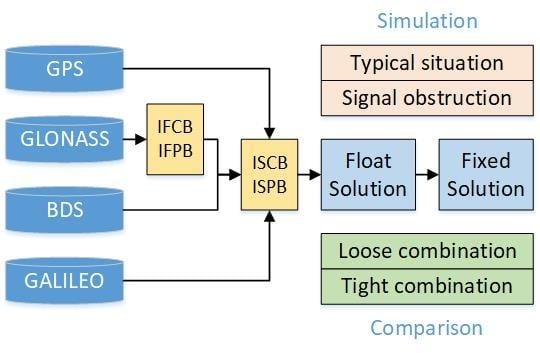
3.1. IFB Calibration

According to Equations (5) and (7), the pseudorange and carrier phase observation equations are biased by IFCB and IFPB, respectively, and these biases must be removed before the subsequent AR.
For the IFCB, Shi et al. [33] analyzed their characteristics and employed both the linear and quadratic frequency functions for different receivers. Zhou et al. [34] used data from 132 International GNSS Service stations, estimated the IFCB for each satellite with a datum constraint, and compared its performance with linear or quadratic polynomial functions. To simplify the model, in this paper only the linear function was adopted, i.e., Δ B r b s = k s · c Δ H r b , where c Δ H r b is the IFCB rate in meters. Thus, the IFCB in Equation (6) can be re-written as:
I F C B r b p q = k q · c Δ H r b k p · c Δ H r b = k p q · c Δ H r b .
In this model, the IFCB rate can be easily determined using the DD pseudorange observation expressions in Equation (5). In the following procedure, the code observables will be significantly down-weighted, and this will hardly cause noticeable bad effects on the solution [16].
For the IFPB, some researchers used the calibration strategy before the positioning process [12,13,14], and others adopted the estimation strategy in the processing procedure [15,16,17]. Since the IFPB has a great impact on the AR, it should be precisely estimated. Herein, we will propose an easy-to-implement method to quickly determine the accurate IFPB value.
As derived from the SD carrier phase observation equation in meters in Equation (3), we can obtain the DD carrier phase observation equation in cycles for the GLONASS as follows:
Δ φ r b p q = Δ ρ r b q λ q Δ ρ r b p λ p Δ N r b p q + f p q · Δ d t r b + Δ b r b p q + Δ ε φ ,
where f p q is the frequency difference between two satellites. Furthermore, the frequency can be expressed as a linear function of k s , i.e.:
f s = f 0 + a k s ,
where f 0 is the central frequency and a is the constant coefficient. For the L1 signal, they are 1602 MHz and 9/16 MHz, respectively. f p q is then transformed to a k p q . Since we know that k s [ 7 ,   6 ] , if the precision of the estimated Δ d t r b can reach 10 ns, the largest bias caused by Δ d t r b will be smaller than 0.08 cycles and the ambiguity rounding can only be affected by the IFPB.
Furthermore, the linear relationship between the IFPB and k s is given as [11]:
λ s · Δ b r b s = k s · c Δ h r b ,
where c Δ h r b is the IFPB rate in meters. Combining Equations (15) and (16), Δ b r b p q can be derived:
Δ b r b p q = k q f q Δ h r b k p f p Δ h r b = f 0 k p q Δ h r b + a ( ( k q ) 2 ( k p ) 2 ) Δ h r b .
Benefitting from the previous research by Wanninger [11], an empirical range of c Δ h r b that is less than 6 cm can be assumed as the tolerance, i.e., Δ h r b   < 0.2 ns. For the single-frequency case, when the condition k p q = ± 1 is satisfied, the bias Δ b r b p q is smaller than 0.322 cycles, and the bias caused by Δ d t r b is further reduced to no more than 0.006 cycles. As a result, for baselines with known coordinates for the base station and rover station, the total bias in Equation (14) will be no more than 0.33 cycles. If we temporarily ignore the effect of the hardware delay, the DD ambiguity can be estimated by directly rounding:
Δ N r b p q = r o u n d ( Δ ρ r b q λ q Δ ρ r b p λ p Δ φ r b p q + k p q a Δ d t r b ) ,
where round(*) means the rounding off operation. In this way, the DD integer ambiguity is determined, and the next step is to calculate the IFPB rate.
It should be mentioned that the efficiency of this algorithm is affected by two factors: the precision of Δ d t r b and the limit of the IFPB rate. If the above limit of 6 cm for IFPB rate is used, the precision of Δ d t r b can be as tolerant as 200 ns. On the other hand, considering there is no guarantee that the above critical value of the IFPB rate is the absolute limit, the IFPB rate that can be supported by our algorithm should be no larger than 9 cm, where the precision of Δ d t r b should not exceed 10 ns. Otherwise, the DD integer ambiguity cannot be fixed to its right value and the algorithm is inapplicable.
According to Equation (16) and the definition of IFPB in Equation (6), the IFPB is expressed in a similar model as the IFCB in Equation (13), i.e., I F P B r b p q = k p q c Δ h r b . From the DD carrier phase observation equation in Equation (5), we can obtain the IFPB rate as follows:
c Δ h r b = ( Δ ϕ r b p q Δ ρ r b p q + λ q Δ N r b p q + ( λ q λ p ) Δ N r b p ) / k p q ,
where the float DD ambiguity is converted to the combination of an integer DD ambiguity Δ N r b p q and the SD ambiguity for the reference satellite Δ N r b p . The initial value of Δ N ˜ r b p can be easily calculated via Equation (3) when the hardware delays are ignored. The bias in the calculated Δ N ˜ r b p will be dramatically reduced due to the mm-level’s coefficient ( λ q λ p ) . If no cycle slip occurs, Δ N r b p remains the same and the IFPB rate can be determined.
Since there may be only a very few DD observables meeting k p q = ± 1 at a single epoch, the obtained IFPB rates may be very noisy. Therefore, a sufficient duration is required to smooth the noisy IFPB rates and achieve a relatively accurate initial value. After the initial IFPB rate is calculated, the bias Δ b r b p q in Equation (17) can thereby be calculated, and all DD ambiguity can then be re-estimated using the corresponding DD carrier phase observables:
Δ N r b p q = r o u n d ( Δ ρ r b q λ q Δ ρ r b p λ p Δ φ r b p q + k p q a Δ d t r b + Δ b r b p q ) .
Similarly, from Equation (19) we can get the IFPB rate again at each epoch using all DD observables, and further obtain a much more accurate value through smoothing. In other word, the IFPB rate is iterated from an initial value to a much more accurate value. The whole procedure is listed in Figure 1.
Before applying the above procedure, some remarks should be made. The first is the inputs, where only the pair of observation data files with known coordinates can be used in our algorithm. The second is the condition difference to calculate the initial and the final IFPB rate. When we use DD observables to determine the DD ambiguity the first time, the condition k p q = ± 1 must be satisfied. However, when we determine the DD ambiguity again after we obtained the initial IFPB rate, all DD observables were utilized to get more calculated IFPB rates and thus a more precise result.
Taking the data in Figure 2 as examples and using the above-proposed method, we obtained the epoch-by-epoch IFCB rates and IFPB rates, which are plotted in Figure 2 The final smoothed IFCB rates, IFPB rates, and corresponding standard deviations (STDs) are listed in Figure 2.
From Figure 2, we can see that the IFB rates were very stable during one day’s observation session for all six baselines; thus, we can calibrate this bias using a pre-estimated value. Meanwhile, the IFPB rates for all baselines with homogeneous receivers were almost normally distributed and the statistical results were close to zero, while the IFB rates for baselines with heterogeneous receivers were obviously biased. Table 2 shows that the IFPB rate for baseline F reached up to 0.03 m. If k p q is larger than 3, the IFPB for this baseline will exceed half cycle, and severely obstruct the subsequent AR. Furthermore, the STD values reflected that by adopting the proposed algorithm, we could obtain a 0.3-m-level IFCB rate and a 0.003-m-level IFPB rate.
After the IFCB and IFPB rates were determined, the IFCB and IFPB can be calculated and expressed as:
{ I F C B r b R = Δ B r b R Δ B r b R 0 = k R · c Δ H r b , I F P B r b R = λ R · Δ b r b R λ R 0 · Δ b r b R 0 = k R · c Δ h r b .
The calculated IFBs were then used for calibration in the tightly combined model.

3.2. ISB Estimation

Taking a tight combination between the GPS and GLONASS as an example, after the IFB is calibrated, the tightly combined observation equations can be re-written as:
{ Δ P r b G R = Δ ρ r b G R + I S C B r b G R + Δ ε P , Δ ϕ r b G R = Δ ρ r b G R ( λ R · Δ N r b R λ G · Δ N r b G ) + I S P B r b G R + Δ ε ϕ .
From Equation (9), and considering the consistency of the hardware delays for all satellite pairs, we can regard both the ISCB and ISPB as short-term constants, which means their values remain unchanged for at least several hours of continuous operation [23,32]. The ISCB can be easily estimated using a least-squares adjustment or Kalman filtering. As for the ISPB, from Equation (22), we find the DD ambiguity has lost its integer nature. Therefore, a transformation similar to Equation (19) is employed to recover the integer nature, and the tightly combined DD carrier phase observation equation is re-expressed as follows:
Δ ϕ r b G R = Δ ρ r b G R λ R Δ N r b G R ( λ R λ G ) Δ N r b G + I S P B r b G R + Δ ε ϕ .
Similarly, the float DD ambiguity is separated into the terms of Δ N r b G R and Δ N r b G , and the initial value of Δ N ˜ r b G can be calculated. If no cycle slip occurs, the reduced bias in the calculated Δ N ˜ r b G will be absorbed into the ISPB.
Since the ISPB and the DD ambiguity terms are also very difficult to separate, they will be regarded as one parameter and estimated together with the coordinates, or directly calculated using the following formula:
Δ N r b G R I S P B r b G R / λ R = ( Δ ρ r b G R Δ ϕ r b G R ( λ R λ G ) Δ N ˜ r b G ) / λ R .
Herein, the geometry can be obtained when we estimate the ISCB. After rounding off, the integer part of the real ISPB is absorbed into the integer DD ambiguity, and the residual is changed to a constant value by multiplying the coefficient λ R / λ R 0 and then taken as the ISPB in cycles. Furthermore, if the determined ISPB is around ±0.5 cycles, one cycle is added to the ISPB around −0.5 cycles to make all results consistent.
For a tight combination between GPS and BDS, there may be a 0.5-cycles inter-satellite type bias in BDS between the geostationary orbit (GEO) satellites and the non-GEO satellites [35], and this bias is corrected in advance. For a tight combination between GPS and Galileo, the overlapping frequency is used and the SD ambiguity term is eliminated, thus the model becomes simple.
The determined ISPBs for each pair of satellites are averaged together to one ISPB value at one epoch. For a short-term observation period, the ISPB can be further smoothed due to its stability to achieve its final value.
Using data in Table 1 and the above method, we obtained the epoch-by-epoch ISCB and ISPB, which are plotted in Figure 3. The final smoothed ISCBs, ISPBs, and corresponding STD values are listed in Table 3.
From Figure 3 and Table 3, we can see that the ISB had a diurnal stability and could be corrected in advance. In addition, the ISCB and ISPB differ from one another, whether homogeneous or heterogeneous receivers are used. The ISCB could be as large as 4 m and the ISPB could reach up to 0.5 cycles. Such large biases will no doubt hamper the subsequent AR and must be removed. In the meantime, the given STD values show that the precision of the estimated ISCB was almost at the same level as the code measurement noise, and the ISCB between GPS and GLONASS was slightly larger than other inter-system pairs. This was reasonable due to the large code noise of GLONASS. As for ISPB, for ultra-short baselines, the precision could be up to 0.015 cycles, and a general precision of 0.03 cycles was achieved.
What is interesting is that for most baselines, the ISPB values between GPS and Galileo were close to zero because of their identical frequency, with the only exception being for baseline F. This indicates that the ISPB may exist even if overlapping frequencies are used in tightly combined systems.

4. Numerical Analysis and Discussion

After the removal of the IFB and ISB, the DD ambiguity can be resolved in both loosely and tightly combined models. In this part, we will conduct some experiments and set three different scenarios to investigate and compare the performance of TC with that of LC using multi-GNSS single-frequency data.
Three different scenarios were set according to the satellite elevation mask and azimuth range to simulate different observation environments, which are shown in Table 4. Case 1 was the typical situation in an open area, case 2 simulated the ambient occlusion with surrounding high buildings, and case 3 simulated the unilateral shade under a block of high buildings.
In the following discussion, we first give the epoch-by-epoch results of baseline A in case 3 as an example. A final comparison of the float solution and fixed solution between TC and LC in all three scenarios will be made subsequently.
Figure 4 gives the usable number of satellites of each system and the position dilution of precision (PDOP) for all four systems. From the figure, we can see that because of signal obstructions, for most of the time, fewer than five satellites can be used for each system, which means efficient precise positioning is difficult to realize if only a single system is used. However, when all satellites are combined, this problem will be solved. This can be inferred from the corresponding PDOP, whose average value was only 2.3.

4.1. Float Solution

In the data processing, we assumed all code precision was 0.3 m, except for GLONASS with 0.45 m, and all carrier phase precision was 0.003 m. Setting the coordinate and ambiguity as unknown parameters and ignoring the integer nature of the ambiguity, the single-epoch float solution was first obtained using a standard least-squares adjustment ahead of the ambiguity fix. The horizontal and vertical positioning biases for the LC model and TC model, along with the corresponding 95% confidence intervals and standard deviations, are shown in Figure 5. The results indicate that the float solution for TC model in both the horizontal and vertical directions had a moderate improvement compared with those for the LC model.
The position root-mean-square errors (RMSEs) in the TC model and LC model using all six baselines under three scenarios and the corresponding improvements were calculated and are listed in Table 5. The results show that in typical situations (case 1), there were few improvements in the positioning errors in the TC model compared with those in the LC model, but in other two situations (cases 2 and 3) with obstructed satellites, obvious decreases in positioning errors were found. The improving percentage is represented as Pi, and the average values for all six baselines exceeded 30% and 15% for cases 2 and 3, respectively.
The results indicate that the performance of the TC model was similar to that of the LC model in open areas, but was superior to the LC model when there were signal obstructions around. In these complex environments, the TC model was a better choice. In the meantime, we also found that cases 2 and 3 had different degrees of influence on the performance of the TC and LC models, where the TC model could reduce the negative impacts more in situations with a high elevation mask.

4.2. Fixed Solution

For single-epoch precise positioning, the unknown integer ambiguity must be determined to acquire the centimeter level’s fixed solution. After the float ambiguity and its variance were obtained in the float solution, the least-squares ambiguity decorrelation adjustment method [36] was employed to search for the integer ambiguity. During the ambiguity validation procedure, both the data-driven R-ratio test and the model-driven success rate [37] were considered, whose empirical thresholds were set as 3.0 and 99%, respectively, in this paper. When both these two values reached or exceeded their thresholds, the ambiguity was regarded as being fixed. Meanwhile, we realized that the ambiguity may be incorrectly fixed. Among the epochs with fixed ambiguities, only when the positioning biases in all three directions were smaller than 0.1 m could the ambiguity be regarded as being correctly fixed.
Based on the above consideration, we defined the ambiguity fixing rate P f i x and ambiguity correctly-fixed rate P c as:
P f i x = N f i x N A l l × 100 % , P c = N c N f i x × 100 % ,
where N A l l is the total epoch number, N f i x is the epoch number of the fixed ambiguity, and N c is the epoch number of the correctly fixed ambiguity.
The test results with the reciprocal values of the R-ratio are plotted in Figure 6. It is clear that more ratio values exceeded the threshold in the TC model than those in the LC model. In other words, in the TC model, more fixed epochs were achieved.
Combining the ratio-test and the AR success rate, we could calculate P f i x for both the LC and TC models under different situations; the results for all six baselines are listed in Table 6. The difference in P f i x between TC and LC is denoted as Δ f i x , i.e., Δ f i x = P f i x ( T C ) P f i x ( L C ) . It shows that P f i x in the LC and TC models were nearly the same in case 1, which means they had a similar performance in normal situations. However, in cases 2 and 3, the TC model outperformed the LC model, where the difference of P f i x could be more than 30%. It is clear that the TC model increased the performance of ambiguity fixing.
Furthermore, by judging whether the ambiguity was correctly fixed, we could calculate P c for both LC and TC models under different situations, whose results for all six baselines are listed in Table 7. The difference in P c between TC and LC is written as Δc. From the table, we can see that just like the results of P f i x , in case 1, we obtained similar correctly fixed ambiguity rates for TC and LC. In cases 2 and 3, the correctly fixed ambiguity rates in the TC model showed a moderate improvement. Considering the remarkable improvement of the ambiguity fixing rate, many more ambiguities were reliably fixed to their correct values. The TC model demonstrated significant advantages in AR in special situations with signal occlusion.
It should be pointed out that in cases 1, 2, and 3 of baseline F, there were six, five, and six epochs when the LC model was unavailable because there was only one usable satellite in the GLONASS and Galileo systems. However, this issue was resolved in the TC model. The only exception was for three epochs in case 3 when there was only one satellite in each system, thus the formed three-DD observation equations could not be used for positioning.
The fixed ambiguity could be taken as a known parameter and the fixed solution could thereby be calculated. Excluding the results with an incorrectly fixed ambiguity, we display the positioning biases in the horizontal and vertical directions for baseline A in case 3 with both LC and TC models in Figure 7. The 95% confidence intervals and standard deviations are also plotted in the figures.
We could hardly find any significant differences between the TC and LC models. Both achieved nearly 1-cm-level positioning results. The results for other baselines and other situations were almost the same and are not given in this paper. Therefore, from the perspective of positioning results, the TC and LC models showed the same level of performance.

4.3. Discussion

The above experimental results indicate an obvious advantage of the TC model in situations with obstructed satellites. Although the TC and LC models gave comparable results in open sky, this was usually not the case for urban residents. The pedestrian on the streets must face a situation under high buildings, where severe signal occlusion inevitably happens and hampers efficient navigation. From the functional models of TC and LC, if the ISBs are calibrated ahead of the positioning, the TC model can provide one more observation equation for each pair of systems, and the degree of freedom becomes large [30]. When the four systems are used together, the redundancy increases to three. In situations with limited tracked satellites, the additional equations can make a positive impact on the AR and positioning performance. That is why better results were achieved in TC model, as shown in Table 5 and Table 6.
Meanwhile, the functional model of TC infers that many more advantages can be acquired if more systems are involved compared with LC. If the regional satellite systems, such as Japanese QZSS and Indian IRNSS, are not taken into account, the integration of GPS, GLONASS, Galileo, and BDS maximizes the performance of a tightly combined solution. Although lots of contributions have been made using the hybrid systems with CDMA signals, it is a pity that in their work, the GLONASS signals are abandoned, maybe due to its FDMA signals and the corresponding IFB. This paper provides a further investigation of precise positioning with all four global navigation satellite systems by considering both IFB and ISB.
Furthermore, as more and more satellites are available, we do not need to resolve all tracked satellites since fixing the full set of ambiguities of multiple constellations may possibly decrease the AR success rate and computational efficiency, and the partial ambiguity resolution (PAR) technique, which resolves a subset of the ambiguities, was suggested to achieve a high success rate [38]. After the selection of an ambiguity set based on a certain strategy, the number of remaining satellites may be not that sufficient. At this moment, the TC model can be applied to ensure the position estimation. Therefore, the combination of the PAR technique and the tightly combined multi-GNSS system will bring about a high AR success rate and ambiguity fixing rate, along with time-saving data processing, regardless of whether the observation environment is in clear-sky or suffers from signal occlusion. This is expected to become a more efficient work pattern in the coming multi-GNSS era.

5. Conclusions

In this paper, we provided a rigorous functional model for tightly combined single-frequency multi-GNSS data. The virtual signal of the constant central frequency in the GLONASS system with a channel number of zero was introduced, and the IFPB and ISPB in GLONASS involving a tightly combined system were re-defined from the hardware delays.
Based on this functional model, we proposed a practical algorithm to estimate the IFB rate and the ISB, and their characteristics were analyzed using six pairs of available single-frequency multi-GNSS data of ultra-short and short baselines. Numerical results confirmed that the IFPB rates for baselines with homogeneous receivers were negligible, while those with heterogeneous receivers should be calibrated. Results also indicated that there may be considerable ISPB even if overlapping frequencies are used in tightly combined systems.
After the removal of the IFB and ISB, a comprehensive performance comparison was made from the float solution to the fixed solution between the TC and LC models. Experiments were conducted to simulate three different observation environments: one is the typical situation and the other two suffer from signal obstruction with high elevation angles or limited azimuths, respectively. From the results, we found that in typical situations, the TC model and LC model had a similar performance in the float solution and AR. However, when the satellite signals were severely obstructed and few satellites could be tracked in a single system, the float solution and ambiguity fixing rates in the LC model were dramatically decreased, while those in the TC model had relatively smaller declines, where the difference in ambiguity fixing rates could be as large as 30%. The correctly fixed ambiguity rates in the TC model also had a moderate improvement of around 10%. Once the ambiguity was fixed, both models achieved a similar positioning accuracy. Summarily, the TC model significantly outperformed the LC model in terms of AR in cases of signal obstruction, though in other cases, they had a similar performance.

Author Contributions

Conceptualization, X.Z. and W.T.; methodology, C.D. and Q.L.; software, Q.L.; validation, Q.L., J.C., and C.G.; formal analysis, C.D.; investigation, C.G.; resources, Q.L.; data curation, J.C.; writing—original draft preparation, Q.L.; writing—review and editing, C.D. and Y.W.; visualization, C.G.; supervision, W.T.; project administration, X.Z.; funding acquisition, C.D. All authors have read and agreed to the published version of the manuscript.

Funding

This research was funded by the National Key Research and Development Program of China (grant no. 2018YFB1305001), National Natural Science Foundation of China (grant nos. 41804028, 41874037), and Joint Fund of Ministry of Education of China for Equipment Pre-research (grant no. 6141A02022372).

Acknowledgments

The ultra-short baselines data were downloaded from the website of the GNSS Research Centre of Curtin University (http://saegnss2.curtin.edu.au/ldc/) and the short baselines data were downloaded from the website of Hong Kong Geodetic Survey Services (http://www.geodetic.gov.hk/sc/geod_services.htm). We are grateful to these organizations for generously and freely sharing these valuable data. In addition, we also thank three anonymous reviewers for their constructive comments that helped to improve the quality of this paper.

Conflicts of Interest

The authors declare no conflict of interest.

References

  1. Lohan, E.S.; Borre, K. Accuracy limits in multi-GNSS. IEEE Trans. Aerosp. Electr. Syst. 2016, 52, 2477–2494. [Google Scholar] [CrossRef]
  2. Pan, Z.; Chai, H.; Kong, Y. Integrating multi-GNSS to improve the performance of precise point positioning. Adv. Space Res. 2017, 60, 2596–2606. [Google Scholar] [CrossRef]
  3. Zhang, W.; Cannon, M.E.; Julien, O.; Alves, P. Investigation of combined GPS/GALILEO cascading ambiguity resolution schemes. In Proceedings of the ION GPS/GNSS 2003, Portland, OR, USA, 9–12 September 2003; pp. 2599–2610. [Google Scholar]
  4. Julien, O.; Alves, P.; Cannon, M.E.; Zhang, W. A tightly coupled GPS/GALILEO combination for improved ambiguity resolution. In Proceedings of the European Navigation Conference (ENC-GNSS’03), Graz, Austria, 22–25 April 2003. [Google Scholar]
  5. GLONASS ICD. GLONASS Interface Control Document, Edition 5.1. 2008. Available online: https://www.unavco.org/help/glossary/docs/ICD_GLONASS_5.1_(2008)_en.pdf (accessed on 24 October 2019).
  6. Dodson, A.H.; Moore, T.; Baker, D.F.; Swann, J.W. Hybrid GPS + GLONASS. GPS Solut. 1999, 3, 32–41. [Google Scholar] [CrossRef]
  7. Wang, J.; Rizos, C.; Stewart, M.P.; Leick, A. GPS and GLONASS integration: Modeling and ambiguity resolution issues. GPS Solut. 2001, 5, 55–64. [Google Scholar] [CrossRef]
  8. Dai, L.; Han, S.; Rizos, C. Performance analysis of integrated GPS/GLONASS carrier phase-based positioning. Geo-Spat. Inf. Sci. 2001, 4, 9–18. [Google Scholar] [CrossRef] [Green Version]
  9. Al-Shaery, A.; Zhang, S.; Lim, S.; Rizos, C. A comparative study of mathematical modelling for GPS/GLONASS real-time kinematic (RTK). In Proceedings of the ION GNSS 2012, Nashville, TN, USA, 17–21 September 2012; pp. 2231–2238. [Google Scholar]
  10. Wanninger, L.; Wallstab-Freitag, S. Combined processing of GPS, GLONASS, and SBAS code phase and carrier phase measurements. In Proceedings of the ION GNSS 2007, Fort Worth, TX, USA, 25–28 September 2007; pp. 866–875. [Google Scholar]
  11. Wanninger, L. Carrier-phase inter-frequency biases of GLONASS receivers. J. Geod. 2012, 86, 139–148. [Google Scholar] [CrossRef] [Green Version]
  12. Boriskin, A.; Zyryanov, G. Algorithms to calibrate and compensate for GLONASS biases in GNSS RTK receivers working with 3rd party networks. In Proceedings of the ION GNSS 2008, Savannah, GA, USA, 16–19 September 2008; pp. 376–384. [Google Scholar]
  13. Yamada, H.; Takasu, T.; Kubo, N.; Yasuda, A. Evaluation and calibration of receiver inter-channel biases for RTK-GPS/GLONASS. In Proceedings of the 23rd ITM of the Satellite Division of ION, Portland, OR, USA, 21–24 September 2010; pp. 1580–1587. [Google Scholar]
  14. Al-Shaery, A.; Zhang, S.; Rizos, C. An enhanced calibration method of GLONASS inter-channel bias for GNSS RTK. GPS Solut. 2013, 17, 165–173. [Google Scholar] [CrossRef]
  15. Banville, S.; Collins, P.; Lahaye, F. GLONASS ambiguity resolution of mixed receiver types without external calibration. GPS Solut. 2013, 17, 275–282. [Google Scholar] [CrossRef]
  16. Tian, Y.; Ge, M.; Neitzel, F. Particle filter-based estimation of inter-frequency phase bias for real-time GLONASS integer ambiguity resolution. J. Geod. 2015, 89, 1145–1158. [Google Scholar] [CrossRef]
  17. Yao, Y.; Hu, M.; Xu, X.; He, Y. GLONASS inter-frequency phase bias rate estimation by single-epoch or Kalman filter algorithm. GPS Solut. 2017, 21, 1871–1882. [Google Scholar] [CrossRef]
  18. Tiberiu, C.; Pany, T.; Eissfeller, B.; Joosten, P.; Verhagen, S. 0.99999999 confidence ambiguity resolution with GPS and Galileo. GPS Solut. 2002, 6, 96–99. [Google Scholar] [CrossRef]
  19. Teunissen, P.J.G.; Odolinski, R.; Odijk, D. Instantaneous BeiDou+GPS RTK positioning with high cut-off elevation angles. J. Geod. 2014, 88, 335–350. [Google Scholar] [CrossRef]
  20. Deng, C.; Tang, W.; Liu, J.; Shi, C. Reliable single-epoch ambiguity resolution for short baselines using combined GPS/BeiDou system. GPS Solut. 2014, 18, 375–386. [Google Scholar] [CrossRef]
  21. Håkansson, M.; Jensen, A.B.O.; Horemuz, M.; Hedling, G. Review of code and phase biases in multi-GNSS positioning. GPS Solut. 2017, 21, 849–860. [Google Scholar] [CrossRef] [Green Version]
  22. Paziewski, J.; Wielgosz, P. Assessment of GPS + Galileo and multi-frequency Galileo single-epoch precise positioning with network corrections. GPS Solut. 2014, 18, 571–579. [Google Scholar] [CrossRef] [Green Version]
  23. Odijk, D.; Teunissen, P.J.G. Characterization of between-receiver GPS-Galileo inter-system biases and their effect on mixed ambiguity resolution. GPS Solut. 2013, 17, 521–533. [Google Scholar] [CrossRef]
  24. Paziewski, J.; Sieradzki, R.; Wielgosz, P. Selected properties of GPS and Galileo-IOV receiver intersystem biases in multi-GNSS data processing. Meas. Sci. Technol. 2015, 26, 95008. [Google Scholar] [CrossRef]
  25. Tian, Y.; Liu, Z.; Ge, M.; Neitzel, F. Multi-dimensional particle filter-based estimation of inter-system phase biases for multi-GNSS real-time integer ambiguity resolution. J. Geod. 2019, 93, 1073–1087. [Google Scholar] [CrossRef]
  26. Gao, W.; Meng, X.; Gao, C.; Pan, S.; Wang, D. Combined GPS and BDS for single-frequency continuous RTK positioning through real-time estimation of differential inter-system biases. GPS Solut. 2018, 22, 20. [Google Scholar] [CrossRef]
  27. Odolinski, R.; Teunissen, P.J.G.; Odijk, D. Combined BDS, Galileo, QZSS and GPS single-frequency RTK. GPS Solut. 2015, 19, 151–163. [Google Scholar] [CrossRef]
  28. Wu, M.; Liu, W.; Wang, W.; Zhang, X. Differential inter-system biases estimation and initial assessment of instantaneous tightly combined RTK with BDS-3, GPS, and Galileo. Remote Sens. 2019, 11, 1430. [Google Scholar] [CrossRef] [Green Version]
  29. Gao, W.; Pan, S.; Gao, C.; Wang, Q.; Shang, R. Tightly combined GPS and GLONASS for RTK positioning with consideration of differential inter-system phase bias. Meas. Sci. Technol. 2019, 30, 54001. [Google Scholar] [CrossRef]
  30. Paziewski, J.; Wielgosz, P. Investigation of some selected strategies for multi-GNSS instantaneous RTK positioning. Adv. Space Res. 2017, 59, 12–23. [Google Scholar] [CrossRef]
  31. Teunissen, P.J.G. GPS carrier phase ambiguity fixing concepts. In GPS for Geodesy; Springer: Berlin/Heidelberg, Germany, 1996; pp. 263–335. [Google Scholar]
  32. Paziewski, J.; Wielgosz, P. Accounting for Galileo–GPS inter-system biases in precise satellite positioning. J. Geod. 2015, 89, 81–93. [Google Scholar] [CrossRef] [Green Version]
  33. Shi, C.; Yi, W.; Song, W.; Lou, Y.; Yao, Y.; Zhang, R. GLONASS pseudorange inter-channel biases and their effects on combined GPS/GLONASS precise point positioning. GPS Solut. 2013, 17, 439–451. [Google Scholar] [CrossRef]
  34. Zhou, F.; Dong, D.; Ge, M.; Li, P.; Wickert, J.; Schuh, H. Simultaneous estimation of GLONASS pseudorange inter-frequency biases in precise point positioning using undifferenced and uncombined observations. GPS Solut. 2018, 22, 19. [Google Scholar] [CrossRef]
  35. Nadarajah, N.; Teunissen, P.J.G.; Sleewaegen, J.; Montenbruck, O. The mixed-receiver BeiDou inter-satellite-type bias and its impact on RTK positioning. GPS Solut. 2015, 19, 357–368. [Google Scholar] [CrossRef]
  36. Teunissen, P.J.G. The least-squares ambiguity decorrelation adjustment: A method for fast GPS integer ambiguity estimation. J. Geod. 1995, 70, 65–82. [Google Scholar] [CrossRef]
  37. Teunissen, P.J.G. The success rate and precision of GPS ambiguities. J. Geod. 2000, 74, 321–326. [Google Scholar] [CrossRef] [Green Version]
  38. Wang, J.; Feng, Y. Reliability of partial ambiguity fixing with multiple GNSS constellations. J. Geod. 2013, 87, 1–14. [Google Scholar] [CrossRef]
Figure 1. Flowchart of the IFPB rate estimation. DD: double-differenced, IFPB: inter-frequency phase bias, OBS: observations.
Remotesensing 12 00285 g001
Figure 2. Estimated inter-frequency bias (IFB) rates in meters: top—inter-frequency code bias (IFCB) rate, bottom—IFPB rate. In the left panels are the results for the ultra-short baselines, where green dots, blue dots, and yellow dots are for baselines A, B, and C, respectively. In the right panels are the results for the short baselines, where green dots, blue dots, and yellow dots are for baselines D, E, and F, respectively. Heterogeneous receivers were used in baselines C and F.
Remotesensing 12 00285 g002
Figure 3. Estimated epoch-by-epoch inter-system bias (ISB): left—inter-system code bias (ISCB), right—inter-system phase bias (ISPB). The up, middle, and bottom panels contain the ISB values between GPS and GLObal NAvigation Satellite System (GLONASS), between GPS and BeiDou Navigation Satellite System (BDS), and between GPS and Galileo, respectively. In the figure, the dots with different colors denote different baselines.
Remotesensing 12 00285 g003
Figure 4. Number of usable satellites in case 3 (green: GPS; violet: GLONASS; blue: BDS; magenta: Galileo) and position dilution of precision (PDOP) values of multi-GNSS (red).
Remotesensing 12 00285 g004
Figure 5. Float solutions with respect to the horizontal biases (a) and the vertical biases (b). Green dots and lines are for the loose combination (LC) and blue are for the tight combination (TC). The ellipsoids in (a) and lines in (b) show the bias within the 95% confidence level.
Remotesensing 12 00285 g005
Figure 6. The reciprocal ratio values in ambiguity resolution (AR). The green and blue dots are for the LC and TC models, respectively. The yellow line is the threshold of ambiguity fixing with respect to the ratio value, where 1/3 was employed. There were 2124 and 2734 epochs when the ratio test was passed for LC and TC models.
Remotesensing 12 00285 g006
Figure 7. Fixed solutions with respect to the horizontal biases (a) and the vertical biases (b). Green dots and lines are for LC and blue dots and lines are for TC. The ellipsoids in (a) and lines in (b) show the bias within a 95% confidence level.
Remotesensing 12 00285 g007
Table 1. Configuration of used static baselines.
TagBaseline NameReceiver TypeDateLength (m)
Base StationRover Station
ACUT2-CUTBTRIMBLE NETR9TRIMBLE NETR91 January4.27
BCUT3-CUCCJAVAD TRE_G3TJAVAD TRE_G3T1 March7.99
CCUT3-CUTAJAVAD TRE_G3TTRIMBLE NETR91 March8.42
DHKWS-HKSSLEICA GR50LEICA GR501 January6812.47
EHKQT-HKLMTRIMBLE NETR9TRIMBLE NETR91 January12,486.21
FHKQT-HKSCTRIMBLE NETR9LEICA GR501 January8183.52
Table 2. Estimated IFCB rates, IFPB rates, and the corresponding standard deviations (STDs) for different baselines.
BaselineABCDEF
IFCB rate (m)−0.0048−0.0544−0.33360.0148−0.02970.1576
STD (m)0.33180.27960.32020.13670.19300.1764
IFPB rate (m)−0.0001−0.0001−0.00400.0000−0.00020.0312
STD (m)0.00180.00050.00060.00170.00300.0029
Table 3. Estimated ISCB, ISPB, and the corresponding STDs between GLONASS/BDS/Galileo and GPS. The symbols “G-R”, “G-C”, and “G-E” in the table mean operation between GPS and GLONASS, between GPS and BDS, and between GPS and Galileo, respectively.
BaselineISCB (m)ISPB (cycle)
G-RG-CG-EG-RG-CG-E
A−0.1624−1.2582−0.0323−0.05150.4706−0.0013
STD-A0.50220.38250.35030.03780.02010.0087
B0.78340.2206−0.0404−0.1605−0.0095−0.0012
STD-B0.61340.34760.54690.02330.01320.0143
C0.64603.44530.46620.31410.5612−0.0007
STD-C0.74220.36780.45790.04140.01580.0143
D0.23390.0017−0.0181−0.10890.4182−0.0037
STD-D0.36550.19640.24800.02660.01690.0216
E−1.19970.45150.3265−0.03540.4248−0.0163
STD-E0.50010.17020.17360.03650.03950.0347
F−0.9774−1.5025−4.11080.10780.18310.5008
STD-F0.43910.20430.21380.04830.03310.0369
Table 4. Three scenarios with different elevation and azimuth masks.
ScenarioCase 1Case 2Case 3
Elevation mask (°)104010
Azimuth range (°)0–3600–360180–360
Table 5. Comparison of RMSEs in the float solution between LC and TC under different scenarios and the corresponding improvements.
TagCase 1Case 2Case 3
LC (m)TC (m)Pi (%)LC (m)TC (m)Pi (%)LC (m)TC (m)Pi (%)
A0.8980.8268.022.4871.87424.652.3171.98314.42
B1.0491.0182.962.9062.53312.842.8722.32319.12
C0.9600.8956.775.2752.17158.842.7972.26818.91
D0.4440.4293.381.2601.11011.901.1251.0447.200
E0.5010.4745.391.2280.97520.601.2951.09515.44
F0.5870.5565.281.6191.27821.062.0801.70917.84
Mean0.7400.7005.432.4631.65732.722.0811.73716.53
Table 6. Comparison of the ambiguity fixing rates between LC and TC under different scenarios and the corresponding differences.
TagCase 1Case 2Case 3
LC (%)TC (%) Δ f i x ( % ) LC (%)TC (%) Δ f i x ( % ) LC (%)TC (%) Δ f i x ( % )
A100.00100.000.0071.0899.5528.4741.9174.6532.74
B99.8699.860.0048.9678.9229.9721.9158.6536.74
C99.9799.970.0061.4983.4021.9123.2369.1745.94
D99.5899.580.0066.3599.2732.9254.3495.7341.39
E74.5872.26−2.3367.8595.7327.8835.6668.4032.74
F89.5186.04−3.4765.2897.8532.5738.4774.2035.73
Mean93.9292.95−0.9763.5092.4528.9535.9273.4737.55
Table 7. Comparison of correctly fixed ambiguity rates between LC and TC under different scenarios and the corresponding differences.
TagCase 1Case 2Case 3
LC (%)TC (%)Δc (%)LC (%)TC (%)Δc (%)LC (%)TC (%)Δc (%)
A96.7096.15−0.5682.8593.4110.5573.7485.4411.71
B97.6498.120.4982.2786.053.7868.7879.0410.26
C97.7896.56−1.2282.5090.177.6861.1479.1217.98
D93.9394.110.1791.9995.493.4979.8190.4610.65
E78.3180.542.2384.2490.716.4861.7375.6313.90
F72.1968.72−3.4679.8484.324.4742.3354.2811.95
Mean89.4289.03−0.3983.9590.036.0864.5977.3312.74

