Sensitivity Analysis of the DART Model for Forest Mensuration with Airborne Laser Scanning


Abstract
1. Introduction
2. The Discrete Anisotropic Radiative Transfer (DART) Model
3. Materials and Methods
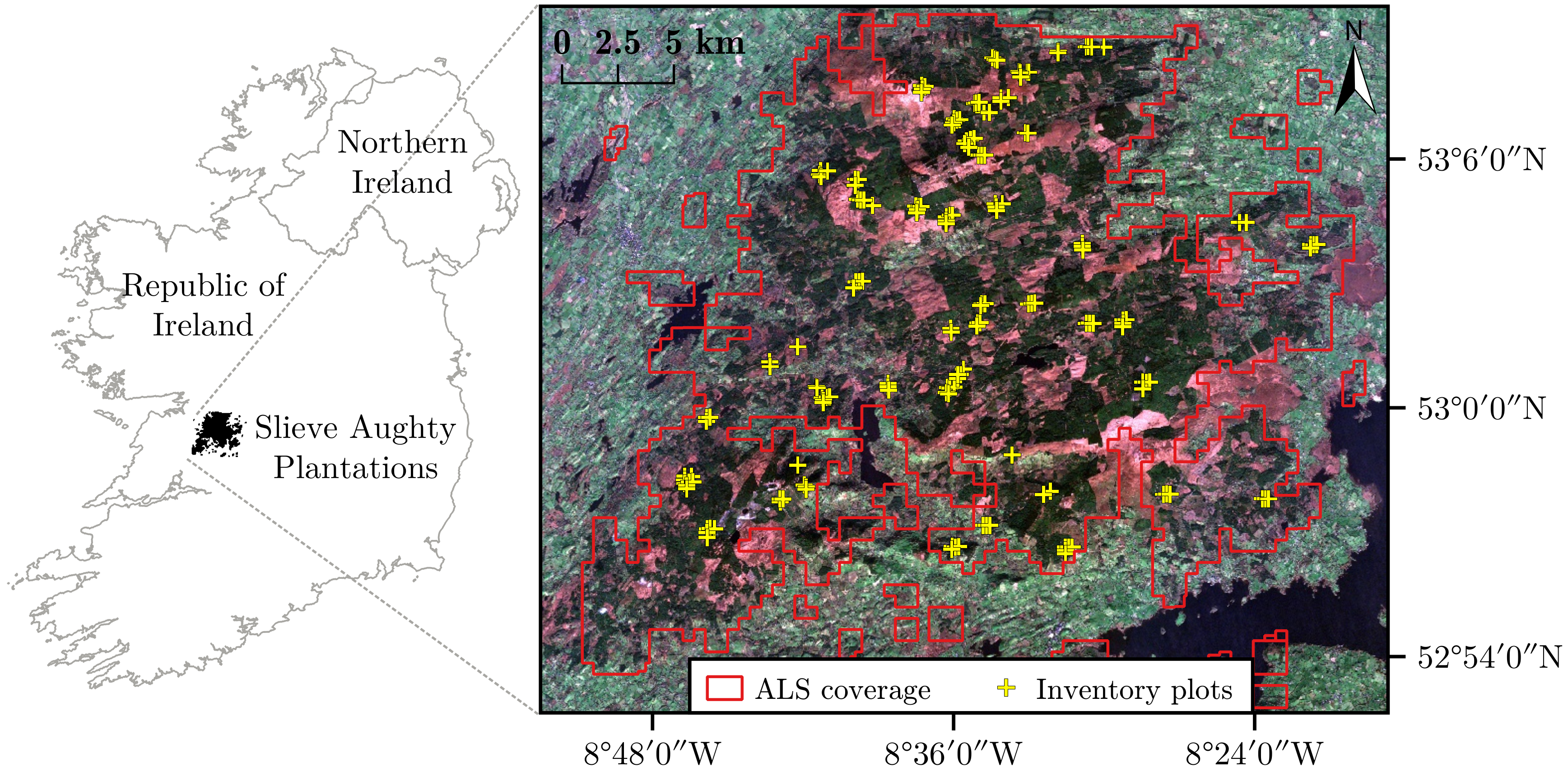
3.1. Reference Data
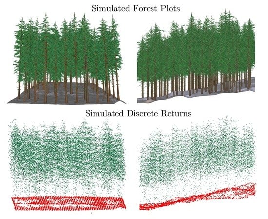
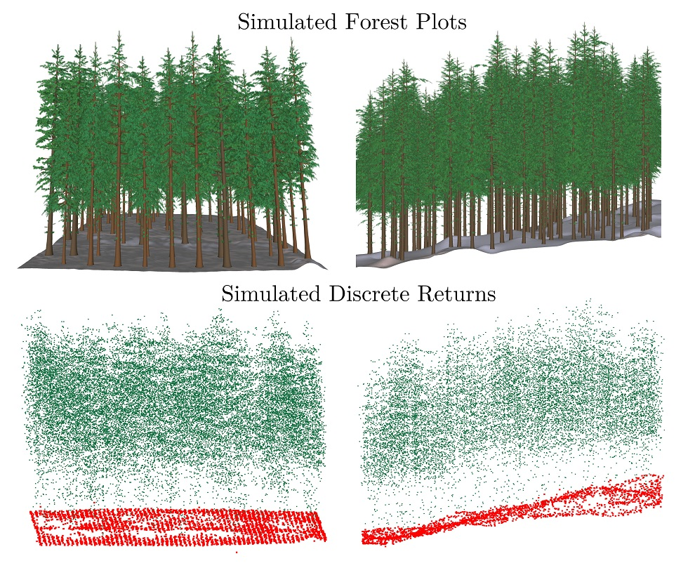
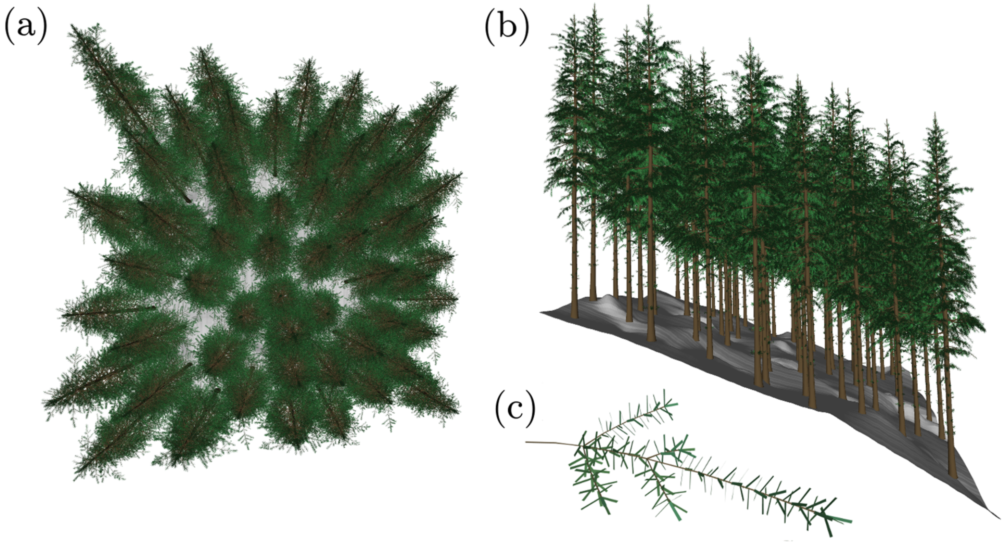
3.2. Forest Plot Reconstruction
3.3. DART Simulation Parameters
3.4. Discrete-Return Metrics
3.5. Sensitivity Analysis
- (i)
- an uncertainty analysis was undertaken to determine the accuracy and precision of discrete-return measurements generated by the DART model,
- (ii)
- a sensitivity analysis was conducted to identify the acquisition parameters that had caused greatest variability in the simulated discrete-return metrics.
4. Results
4.1. Uncertainty Analysis
4.2. Sensitivity Analysis
5. Discussion
5.1. Simulation Accuracy
5.2. Precision of ALS Metrics
5.3. Impact of Acquisition Parameters
6. Conclusions
Author Contributions
Funding
Acknowledgments
Conflicts of Interest
Abbreviations
| ALS | Airborne Laser Scanning |
| DART | The Discrete Anisotropic Radiative Transfer model |
| DBH | Tree diameter at breast height (1.3 m) |
| LiDAR | Light Detection and Ranging |
| MAPE | Mean Absolute Percentage Error |
| PRF | Pulse Repetition Frequency |
| RMSE | Root-Mean-Square Error |
References
- McRoberts, R.E.; Tomppo, E.O. Remote sensing support for national forest inventories. Remote Sens. Environ. 2007, 110, 412–419. [Google Scholar] [CrossRef]
- Barrett, F.; McRoberts, R.E.; Tomppo, E.; Cienciala, E.; Waser, L.T. A questionnaire-based review of the operational use of remotely sensed data by national forest inventories. Remote Sens. Environ. 2016, 174, 279–289. [Google Scholar] [CrossRef]
- White, J.C.; Coops, N.C.; Wulder, M.A.; Vastaranta, M.; Hilker, T.; Tompalski, P. Remote sensing technologies for enhancing forest inventories: A review. Can. J. Remote Sens. 2016, 42, 619–641. [Google Scholar] [CrossRef]
- Hyyppä, J.; Hyyppä, H.; Leckie, D.; Gougeon, F.; Yu, X.; Maltamo, M. Review of methods of small-footprint airborne laser scanning for extracting forest inventory data in boreal forests. Int. J. Remote Sens. 2008, 29, 1339–1366. [Google Scholar] [CrossRef]
- Montaghi, A.; Corona, P.; Dalponte, M.; Gianelle, D.; Chirici, G.; Olsson, H. Airborne laser scanning of forest resources: An overview of research in Italy as a commentary case study. Int. J. Appl. Earth Obs. Geoinf. 2013, 23, 288–300. [Google Scholar] [CrossRef]
- Næsset, E. Area-based inventory in Norway—From innovation to an operational reality. In Forestry Applications of Airborne Laser Scanning; Springer: Berlin/Heidelberg, Germany, 2014; pp. 215–240. [Google Scholar]
- Nilsson, M.; Nordkvist, K.; Jonzén, J.; Lindgren, N.; Axensten, P.; Wallerman, J.; Egberth, M.; Larsson, S.; Nilsson, L.; Eriksson, J.; et al. A nationwide forest attribute map of Sweden predicted using airborne laser scanning data and field data from the National Forest Inventory. Remote Sens. Environ. 2017, 194, 447–454. [Google Scholar] [CrossRef]
- Naesset, E. Determination of mean tree height of forest stands using airborne laser scanner data. ISPRS J. Photogramm. Remote Sens. 1997, 52, 49–56. [Google Scholar] [CrossRef]
- Means, J.E.; Acker, S.A.; Harding, D.J.; Blair, J.B.; Lefsky, M.A.; Cohen, W.B.; Harmon, M.E.; McKee, W.A. Use of large-footprint scanning airborne lidar to estimate forest stand characteristics in the Western Cascades of Oregon. Remote Sens. Environ. 1999, 67, 298–308. [Google Scholar] [CrossRef]
- Andersen, H.E.; Reutebuch, S.E.; McGaughey, R.J. A rigorous assessment of tree height measurements obtained using airborne lidar and conventional field methods. Can. J. Remote Sens. 2006, 32, 355–366. [Google Scholar] [CrossRef]
- Gobakken, T.; Næsset, E. Estimation of diameter and basal area distributions in coniferous forest by means of airborne laser scanner data. Scand. J. For. Res. 2004, 19, 529–542. [Google Scholar] [CrossRef]
- Salas, C.; Ene, L.; Gregoire, T.G.; Næsset, E.; Gobakken, T. Modelling tree diameter from airborne laser scanning derived variables: A comparison of spatial statistical models. Remote Sens. Environ. 2010, 114, 1277–1285. [Google Scholar] [CrossRef]
- Korhonen, L.; Korpela, I.; Heiskanen, J.; Maltamo, M. Airborne discrete-return LIDAR data in the estimation of vertical canopy cover, angular canopy closure and leaf area index. Remote Sens. Environ. 2011, 115, 1065–1080. [Google Scholar] [CrossRef]
- Armston, J.; Disney, M.; Lewis, P.; Scarth, P.; Phinn, S.; Lucas, R.; Bunting, P.; Goodwin, N. Direct retrieval of canopy gap probability using airborne waveform lidar. Remote Sens. Environ. 2013, 134, 24–38. [Google Scholar] [CrossRef]
- Peduzzi, A.; Wynne, R.H.; Fox, T.R.; Nelson, R.F.; Thomas, V.A. Estimating leaf area index in intensively managed pine plantations using airborne laser scanner data. For. Ecol. Manag. 2012, 270, 54–65. [Google Scholar] [CrossRef]
- Pearse, G.D.; Morgenroth, J.; Watt, M.S.; Dash, J.P. Optimising prediction of forest leaf area index from discrete airborne lidar. Remote Sens. Environ. 2017, 200, 220–239. [Google Scholar] [CrossRef]
- Holmgren, J.; Nilsson, M.; Olsson, H. Estimation of tree height and stem volume on plots using airborne laser scanning. For. Sci. 2003, 49, 419–428. [Google Scholar]
- Hollaus, M.; Dorigo, W.; Wagner, W.; Schadauer, K.; Höfle, B.; Maier, B. Operational wide-area stem volume estimation based on airborne laser scanning and national forest inventory data. Int. J. Remote Sens. 2009, 30, 5159–5175. [Google Scholar] [CrossRef]
- Popescu, S.C. Estimating biomass of individual pine trees using airborne lidar. Biomass Bioenergy 2007, 31, 646–655. [Google Scholar] [CrossRef]
- Næsset, E.; Gobakken, T. Estimation of above-and below-ground biomass across regions of the boreal forest zone using airborne laser. Remote Sens. Environ. 2008, 112, 3079–3090. [Google Scholar] [CrossRef]
- Patenaude, G.; Hill, R.; Milne, R.; Gaveau, D.; Briggs, B.; Dawson, T. Quantifying forest above ground carbon content using LiDAR remote sensing. Remote Sens. Environ. 2004, 93, 368–380. [Google Scholar] [CrossRef]
- Asner, G.P.; Mascaro, J.; Muller-Landau, H.C.; Vieilledent, G.; Vaudry, R.; Rasamoelina, M.; Hall, J.S.; Van Breugel, M. A universal airborne LiDAR approach for tropical forest carbon mapping. Oecologia 2012, 168, 1147–1160. [Google Scholar] [CrossRef] [PubMed]
- Van Leeuwen, M.; Nieuwenhuis, M. Retrieval of forest structural parameters using LiDAR remote sensing. Eur. J. For. Res. 2010, 129, 749–770. [Google Scholar] [CrossRef]
- Yu, X.; Hyyppä, J.; Vastaranta, M.; Holopainen, M.; Viitala, R. Predicting individual tree attributes from airborne laser point clouds based on the random forests technique. ISPRS J. Photogramm. Remote Sens. 2011, 66, 28–37. [Google Scholar] [CrossRef]
- Penner, M.; Pitt, D.; Woods, M. Parametric vs. nonparametric LiDAR models for operational forest inventory in boreal Ontario. Can. J. Remote Sens. 2013, 39, 426–443. [Google Scholar]
- Brosofske, K.D.; Froese, R.E.; Falkowski, M.J.; Banskota, A. A review of methods for mapping and prediction of inventory attributes for operational forest management. For. Sci. 2014, 60, 733–756. [Google Scholar] [CrossRef]
- Xu, C.; Manley, B.; Morgenroth, J. Evaluation of modelling approaches in predicting forest volume and stand age for small-scale plantation forests in New Zealand with RapidEye and LiDAR. Int. J. Appl. Earth Obs. Geoinf. 2018, 73, 386–396. [Google Scholar] [CrossRef]
- Boudreau, J.; Nelson, R.F.; Margolis, H.A.; Beaudoin, A.; Guindon, L.; Kimes, D.S. Regional aboveground forest biomass using airborne and spaceborne LiDAR in Québec. Remote Sens. Environ. 2008, 112, 3876–3890. [Google Scholar] [CrossRef]
- Tsui, O.W.; Coops, N.C.; Wulder, M.A.; Marshall, P.L. Integrating airborne LiDAR and space-borne radar via multivariate kriging to estimate above-ground biomass. Remote Sens. Environ. 2013, 139, 340–352. [Google Scholar] [CrossRef]
- Wilkes, P.; Jones, S.; Suarez, L.; Mellor, A.; Woodgate, W.; Soto-Berelov, M.; Haywood, A.; Skidmore, A. Mapping forest canopy height across large areas by upscaling ALS estimates with freely available satellite data. Remote Sens. 2015, 7, 12563–12587. [Google Scholar] [CrossRef]
- Hudak, A.T.; Lefsky, M.A.; Cohen, W.B.; Berterretche, M. Integration of lidar and Landsat ETM+ data for estimating and mapping forest canopy height. Remote Sens. Environ. 2002, 82, 397–416. [Google Scholar] [CrossRef]
- Asner, G.P. Tropical forest carbon assessment: Integrating satellite and airborne mapping approaches. Environ. Res. Lett. 2009, 4, 034009. [Google Scholar] [CrossRef]
- Wulder, M.A.; White, J.C.; Nelson, R.F.; Næsset, E.; Ørka, H.O.; Coops, N.C.; Hilker, T.; Bater, C.W.; Gobakken, T. Lidar sampling for large-area forest characterization: A review. Remote. Sens. Environ. 2012, 121, 196–209. [Google Scholar] [CrossRef]
- Xu, C.; Morgenroth, J.; Manley, B. Integrating data from discrete return airborne LiDAR and optical sensors to enhance the accuracy of forest description: A review. Curr. For. Rep. 2015, 1, 206–219. [Google Scholar] [CrossRef]
- Wehr, A. LiDAR systems and calibration. In Topographic Laser Ranging and Scanning; CRC Press: Boca Raton, FL, USA, 2008; pp. 147–190. [Google Scholar]
- Chasmer, L.; Hopkinson, C.; Treitz, P. Investigating laser pulse penetration through a conifer canopy by integrating airborne and terrestrial lidar. Can. J. Remote Sens. 2006, 32, 116–125. [Google Scholar] [CrossRef]
- Hilker, T.; van Leeuwen, M.; Coops, N.C.; Wulder, M.A.; Newnham, G.J.; Jupp, D.L.; Culvenor, D.S. Comparing canopy metrics derived from terrestrial and airborne laser scanning in a Douglas-fir dominated forest stand. Trees 2010, 24, 819–832. [Google Scholar] [CrossRef]
- Pirotti, F. Analysis of full-waveform LiDAR data for forestry applications: A review of investigations and methods. IForest-Biogeosci. For. 2011, 4, 100–106. [Google Scholar] [CrossRef]
- Hancock, S.; Anderson, K.; Disney, M.; Gaston, K.J. Measurement of fine-spatial-resolution 3D vegetation structure with airborne waveform lidar: Calibration and validation with voxelised terrestrial lidar. Remote Sens. Environ. 2017, 188, 37–50. [Google Scholar] [CrossRef]
- Wagner, W.; Ullrich, A.; Ducic, V.; Melzer, T.; Studnicka, N. Gaussian decomposition and calibration of a novel small-footprint full-waveform digitising airborne laser scanner. ISPRS J. Photogramm. Remote Sens. 2006, 60, 100–112. [Google Scholar] [CrossRef]
- Reitberger, J.; Krzystek, P.; Stilla, U. Analysis of full waveform LIDAR data for the classification of deciduous and coniferous trees. Int. J. Remote Sens. 2008, 29, 1407–1431. [Google Scholar] [CrossRef]
- Anderson, K.; Hancock, S.; Disney, M.; Gaston, K.J. Is waveform worth it? A comparison of LiDAR approaches for vegetation and landscape characterization. Remote Sens. Ecol. Conserv. 2016, 2, 5–15. [Google Scholar] [CrossRef]
- Lindberg, E.; Olofsson, K.; Holmgren, J.; Olsson, H. Estimation of 3D vegetation structure from waveform and discrete return airborne laser scanning data. Remote Sens. Environ. 2012, 118, 151–161. [Google Scholar] [CrossRef]
- Vaughn, N.R.; Moskal, L.M.; Turnblom, E.C. Tree species detection accuracies using discrete point lidar and airborne waveform lidar. Remote Sens. 2012, 4, 377–403. [Google Scholar] [CrossRef]
- Sumnall, M.J.; Hill, R.A.; Hinsley, S.A. Comparison of small-footprint discrete return and full waveform airborne LiDAR data for estimating multiple forest variables. Remote Sens. Environ. 2016, 173, 214–223. [Google Scholar] [CrossRef]
- Brown, C.; Boyd, D.; Sjögersten, S.; Clewley, D.; Evers, S.; Aplin, P. Tropical peatland vegetation structure and biomass: Optimal exploitation of airborne laser scanning. Remote Sens. 2018, 10, 671. [Google Scholar] [CrossRef]
- Corona, P.; Fattorini, L. Area-based lidar-assisted estimation of forest standing volume. Can. J. For. Res. 2008, 38, 2911–2916. [Google Scholar] [CrossRef]
- White, J.C.; Wulder, M.A.; Varhola, A.; Vastaranta, M.; Coops, N.C.; Cook, B.D.; Pitt, D.; Woods, M. A best practices guide for generating forest inventory attributes from airborne laser scanning data using an area-based approach. For. Chron. 2013, 89, 722–723. [Google Scholar] [CrossRef]
- Hyyppa, J.; Kelle, O.; Lehikoinen, M.; Inkinen, M. A segmentation-based method to retrieve stem volume estimates from 3-D tree height models produced by laser scanners. IEEE Trans. Geosci. Remote Sens. 2001, 39, 969–975. [Google Scholar] [CrossRef]
- Breidenbach, J.; Astrup, R. The semi-individual tree crown approach. In Forestry Applications of Airborne Laser Scanning; Springer: Berlin/Heidelberg, Germany, 2014; pp. 113–133. [Google Scholar]
- Zhen, Z.; Quackenbush, L.; Zhang, L. Trends in automatic individual tree crown detection and delineation—Evolution of LiDAR data. Remote Sens. 2016, 8, 333. [Google Scholar] [CrossRef]
- Næsset, E.; Gobakken, T. Estimating forest growth using canopy metrics derived from airborne laser scanner data. Remote Sens. Environ. 2005, 96, 453–465. [Google Scholar] [CrossRef]
- Maltamo, M.; Eerikäinen, K.; Packalén, P.; Hyyppä, J. Estimation of stem volume using laser scanning-based canopy height metrics. Forestry 2006, 79, 217–229. [Google Scholar] [CrossRef]
- Cao, L.; Coops, N.; Hermosilla, T.; Innes, J.; Dai, J.; She, G. Using small-footprint discrete and full-waveform airborne LiDAR metrics to estimate total biomass and biomass components in subtropical forests. Remote Sens. 2014, 6, 7110–7135. [Google Scholar] [CrossRef]
- Bouvier, M.; Durrieu, S.; Fournier, R.A.; Renaud, J.P. Generalizing predictive models of forest inventory attributes using an area-based approach with airborne LiDAR data. Remote Sens. Environ. 2015, 156, 322–334. [Google Scholar] [CrossRef]
- Maltamo, M.; Bollandsås, O.; Næsset, E.; Gobakken, T.; Packalén, P. Different plot selection strategies for field training data in ALS-assisted forest inventory. Forestry 2010, 84, 23–31. [Google Scholar] [CrossRef]
- Dalponte, M.; Martinez, C.; Rodeghiero, M.; Gianelle, D. The role of ground reference data collection in the prediction of stem volume with LiDAR data in mountain areas. ISPRS J. Photogramm. Remote Sens. 2011, 66, 787–797. [Google Scholar] [CrossRef]
- Ruiz, L.; Hermosilla, T.; Mauro, F.; Godino, M. Analysis of the influence of plot size and LiDAR density on forest structure attribute estimates. Forests 2014, 5, 936–951. [Google Scholar] [CrossRef]
- Mauya, E.W.; Hansen, E.H.; Gobakken, T.; Bollandsås, O.M.; Malimbwi, R.E.; Næsset, E. Effects of field plot size on prediction accuracy of aboveground biomass in airborne laser scanning-assisted inventories in tropical rain forests of Tanzania. Carbon Balance Manag. 2015, 10, 10. [Google Scholar] [CrossRef] [PubMed]
- Treitz, P.; Lim, K.; Woods, M.; Pitt, D.; Nesbitt, D.; Etheridge, D. LiDAR sampling density for forest resource inventories in Ontario, Canada. Remote Sens. 2012, 4, 830–848. [Google Scholar] [CrossRef]
- Jakubowski, M.K.; Guo, Q.; Kelly, M. Tradeoffs between lidar pulse density and forest measurement accuracy. Remote Sens. Environ. 2013, 130, 245–253. [Google Scholar] [CrossRef]
- Watt, M.S.; Meredith, A.; Watt, P.; Gunn, A. The influence of LiDAR pulse density on the precision of inventory metrics in young unthinned Douglas-fir stands during initial and subsequent LiDAR acquisitions. N. Z. J. For. Sci. 2014, 44, 18. [Google Scholar] [CrossRef]
- Morsdorf, F.; Frey, O.; Meier, E.; Itten, K.I.; Allgöwer, B. Assessment of the influence of flying altitude and scan angle on biophysical vegetation products derived from airborne laser scanning. Int. J. Remote Sens. 2008, 29, 1387–1406. [Google Scholar] [CrossRef]
- Tinkham, W.T.; Smith, A.M.; Hoffman, C.; Hudak, A.T.; Falkowski, M.J.; Swanson, M.E.; Gessler, P.E. Investigating the influence of LiDAR ground surface errors on the utility of derived forest inventories. Can. J. For. Res. 2012, 42, 413–422. [Google Scholar] [CrossRef]
- Disney, M.I.; Kalogirou, V.; Lewis, P.; Prieto-Blanco, A.; Hancock, S.; Pfeifer, M. Simulating the impact of discrete-return lidar system and survey characteristics over young conifer and broadleaf forests. Remote Sens. Environ. 2010, 114, 1546–1560. [Google Scholar] [CrossRef]
- Næsset, E. Effects of different sensors, flying altitudes, and pulse repetition frequencies on forest canopy metrics and biophysical stand properties derived from small-footprint airborne laser data. Remote Sens. Environ. 2009, 113, 148–159. [Google Scholar] [CrossRef]
- Keränen, J.; Maltamo, M.; Packalen, P. Effect of flying altitude, scanning angle and scanning mode on the accuracy of ALS based forest inventory. Int. J. Appl. Earth Obs. Geoinf. 2016, 52, 349–360. [Google Scholar] [CrossRef]
- Næsset, E.; Bollandsås, O.M.; Gobakken, T. Comparing regression methods in estimation of biophysical properties of forest stands from two different inventories using laser scanner data. Remote Sens. Environ. 2005, 94, 541–553. [Google Scholar] [CrossRef]
- Bater, C.W.; Wulder, M.A.; Coops, N.C.; Nelson, R.F.; Hilker, T.; Nasset, E. Stability of sample-based scanning-LiDAR-derived vegetation metrics for forest monitoring. IEEE Trans. Geosci. Remote Sens. 2011, 49, 2385–2392. [Google Scholar] [CrossRef]
- Wallace, L.; Musk, R.; Lucieer, A. An assessment of the repeatability of automatic forest inventory metrics derived from UAV-borne laser scanning data. IEEE Trans. Geosci. Remote Sens. 2014, 52, 7160–7169. [Google Scholar] [CrossRef]
- Hopkinson, C.; Chasmer, L.; Gynan, C.; Mahoney, C.; Sitar, M. Multisensor and multispectral lidar characterization and classification of a forest environment. Can. J. Remote Sens. 2016, 42, 501–520. [Google Scholar] [CrossRef]
- Næsset, E. Effects of different flying altitudes on biophysical stand properties estimated from canopy height and density measured with a small-footprint airborne scanning laser. Remote. Sens. Environ. 2004, 91, 243–255. [Google Scholar] [CrossRef]
- Goodwin, N.R.; Coops, N.C.; Culvenor, D.S. Assessment of forest structure with airborne LiDAR and the effects of platform altitude. Remote Sens. Environ. 2006, 103, 140–152. [Google Scholar] [CrossRef]
- Chasmer, L.; Hopkinson, C.; Smith, B.; Treitz, P. Examining the influence of changing laser pulse repetition frequencies on conifer forest canopy returns. Photogramm. Eng. Remote Sens. 2006, 72, 1359–1367. [Google Scholar] [CrossRef]
- Hopkinson, C. The influence of flying altitude, beam divergence, and pulse repetition frequency on laser pulse return intensity and canopy frequency distribution. Can. J. Remote Sens. 2007, 33, 312–324. [Google Scholar] [CrossRef]
- Zimble, D.A.; Evans, D.L.; Carlson, G.C.; Parker, R.C.; Grado, S.C.; Gerard, P.D. Characterizing vertical forest structure using small-footprint airborne LiDAR. Remote Sens. Environ. 2003, 87, 171–182. [Google Scholar] [CrossRef]
- Yu, X.; Hyyppä, J.; Hyyppä, H.; Maltamo, M. Effects of flight altitude on tree height estimation using airborne laser scanning. In Proceedings of the Laser Scanners for Forest and Landscape Assessment—Instruments, Processing Methods and Applications, Freiburg, Germany, 3–6 October 2004; pp. 2–6. [Google Scholar]
- Takahashi, T.; Awaya, Y.; Hirata, Y.; Furuya, N.; Sakai, T.; Sakai, A. Effects of flight altitude on LiDAR-derived tree heights in mountainous forests with poor laser penetration rates. Photogramm. J. Finl. 2008, 21, 86–96. [Google Scholar]
- Montealegre, A.; Lamelas, M.; Riva, J. Interpolation routines assessment in ALS-derived digital elevation models for forestry applications. Remote Sens. 2015, 7, 8631–8654. [Google Scholar] [CrossRef]
- Lim, K.; Hopkinson, C.; Treitz, P. Examining the effects of sampling point densities on laser canopy height and density metrics. For. Chron. 2008, 84, 876–885. [Google Scholar] [CrossRef]
- Roussel, J.R.; Caspersen, J.; Béland, M.; Thomas, S.; Achim, A. Removing bias from LiDAR-based estimates of canopy height: Accounting for the effects of pulse density and footprint size. Remote Sens. Environ. 2017, 198, 1–16. [Google Scholar] [CrossRef]
- Magnusson, M.; Fransson, J.E.; Holmgren, J. Effects on estimation accuracy of forest variables using different pulse density of laser data. For. Sci. 2007, 53, 619–626. [Google Scholar]
- Gobakken, T.; Næsset, E. Assessing effects of laser point density, ground sampling intensity, and field sample plot size on biophysical stand properties derived from airborne laser scanner data. Can. J. For. Res. 2008, 38, 1095–1109. [Google Scholar] [CrossRef]
- Thomas, V.; Treitz, P.; McCaughey, J.; Morrison, I. Mapping stand-level forest biophysical variables for a mixedwood boreal forest using lidar: An examination of scanning density. Can. J. For. Res. 2006, 36, 34–47. [Google Scholar] [CrossRef]
- Zheng, G.; Ma, L.; Eitel, J.U.; He, W.; Magney, T.S.; Moskal, L.M.; Li, M. Retrieving directional gap fraction, extinction coefficient, and effective leaf area index by incorporating scan angle information from discrete aerial lidar data. IEEE Trans. Geosci. Remote Sens. 2016, 55, 577–590. [Google Scholar] [CrossRef]
- Liu, J.; Skidmore, A.K.; Jones, S.; Wang, T.; Heurich, M.; Zhu, X.; Shi, Y. Large off-nadir scan angle of airborne LiDAR can severely affect the estimates of forest structure metrics. ISPRS J. Photogramm. Remote Sens. 2018, 136, 13–25. [Google Scholar] [CrossRef]
- North, P.; Rosette, J.; Suárez, J.; Los, S. A Monte Carlo radiative transfer model of satellite waveform LiDAR. Int. J. Remote Sens. 2010, 31, 1343–1358. [Google Scholar] [CrossRef]
- Hovi, A.; Korpela, I. Real and simulated waveform-recording LiDAR data in juvenile boreal forest vegetation. Remote Sens. Environ. 2014, 140, 665–678. [Google Scholar] [CrossRef]
- Disney, M.; Lewis, P.; North, P. Monte Carlo ray tracing in optical canopy reflectance modelling. Remote Sens. Rev. 2000, 18, 163–196. [Google Scholar] [CrossRef]
- Morsdorf, F.; Nichol, C.; Malthus, T.; Woodhouse, I.H. Assessing forest structural and physiological information content of multi-spectral LiDAR waveforms by radiative transfer modelling. Remote Sens. Environ. 2009, 113, 2152–2163. [Google Scholar] [CrossRef]
- Rosette, J.; North, P.; Suarez, J.; Los, S. Uncertainty within satellite LiDAR estimations of vegetation and topography. Int. J. Remote Sens. 2010, 31, 1325–1342. [Google Scholar] [CrossRef]
- Hancock, S.; Disney, M.; Muller, J.P.; Lewis, P.; Foster, M. A threshold insensitive method for locating the forest canopy top with waveform lidar. Remote Sens. Environ. 2011, 115, 3286–3297. [Google Scholar] [CrossRef]
- Rosette, J.; North, P.R.; Rubio-Gil, J.; Cook, B.; Los, S.; Suarez, J.; Sun, G.; Ranson, J.; Blair, J.B. Evaluating prospects for improved forest parameter retrieval from satellite LiDAR using a physically-based radiative transfer model. IEEE J. Sel. Top. Appl. Earth Obs. Remote Sens. 2013, 6, 45–53. [Google Scholar] [CrossRef]
- Koetz, B.; Morsdorf, F.; Sun, G.; Ranson, K.J.; Itten, K.; Allgower, B. Inversion of a lidar waveform model for forest biophysical parameter estimation. IEEE Geosci. Remote Sens. Lett. 2006, 3, 49–53. [Google Scholar] [CrossRef]
- Ma, H.; Song, J.; Wang, J. Forest canopy LAI and vertical FAVD profile inversion from airborne full-waveform LiDAR data based on a radiative transfer model. Remote Sens. 2015, 7, 1897–1914. [Google Scholar] [CrossRef]
- Detto, M.; Asner, G.P.; Muller-Landau, H.C.; Sonnentag, O. Spatial variability in tropical forest leaf area density from multireturn lidar and modeling. J. Geophys. Res. Biogeosci. 2015, 120, 294–309. [Google Scholar] [CrossRef]
- Bye, I.; North, P.R.; Los, S.; Kljun, N.; Rosette, J.; Hopkinson, C.; Chasmer, L.; Mahoney, C. Estimating forest canopy parameters from satellite waveform LiDAR by inversion of the FLIGHT three-dimensional radiative transfer model. Remote Sens. Environ. 2017, 188, 177–189. [Google Scholar] [CrossRef]
- Calders, K.; Lewis, P.; Disney, M.; Verbesselt, J.; Herold, M. Investigating assumptions of crown archetypes for modelling LiDAR returns. Remote Sens. Environ. 2013, 134, 39–49. [Google Scholar] [CrossRef]
- Van Leeuwen, M.; Coops, N.C.; Hilker, T.; Wulder, M.A.; Newnham, G.J.; Culvenor, D.S. Automated reconstruction of tree and canopy structure for modeling the internal canopy radiation regime. Remote Sens. Environ. 2013, 136, 286–300. [Google Scholar] [CrossRef]
- Widlowski, J.L.; Côté, J.F.; Béland, M. Abstract tree crowns in 3D radiative transfer models: Impact on simulated open-canopy reflectances. Remote Sens. Environ. 2014, 142, 155–175. [Google Scholar] [CrossRef]
- Ligot, G.; Balandier, P.; Courbaud, B.; Claessens, H. Forest radiative transfer models: Which approach for which application? Can. J. For. Res. 2014, 44, 391–403. [Google Scholar] [CrossRef]
- Côté, J.F.; Widlowski, J.L.; Fournier, R.A.; Verstraete, M.M. The structural and radiative consistency of three-dimensional tree reconstructions from terrestrial lidar. Remote Sens. Environ. 2009, 113, 1067–1081. [Google Scholar] [CrossRef]
- Hancock, S.; Lewis, P.; Foster, M.; Disney, M.; Muller, J.P. Measuring forests with dual wavelength lidar: A simulation study over topography. Agric. For. Meteorol. 2012, 161, 123–133. [Google Scholar] [CrossRef]
- Montesano, P.; Rosette, J.; Sun, G.; North, P.; Nelson, R.; Dubayah, R.; Ranson, K.; Kharuk, V. The uncertainty of biomass estimates from modeled ICESat-2 returns across a boreal forest gradient. Remote Sens. Environ. 2015, 158, 95–109. [Google Scholar] [CrossRef]
- Ni-Meister, W.; Yang, W.; Lee, S.; Strahler, A.H.; Zhao, F. Validating modeled lidar waveforms in forest canopies with airborne laser scanning data. Remote Sens. Environ. 2018, 204, 229–243. [Google Scholar] [CrossRef]
- Holmgren, J.; Nilsson, M.; Olsson, H. Simulating the effects of lidar scanning angle for estimation of mean tree height and canopy closure. Can. J. Remote Sens. 2003, 29, 623–632. [Google Scholar] [CrossRef]
- Lovell, J.; Jupp, D.; Newnham, G.; Coops, N.; Culvenor, D. Simulation study for finding optimal lidar acquisition parameters for forest height retrieval. For. Ecol. Manag. 2005, 214, 398–412. [Google Scholar] [CrossRef]
- Goodwin, N.; Coops, N.; Culvenor, D. Development of a simulation model to predict LiDAR interception in forested environments. Remote Sens. Environ. 2007, 111, 481–492. [Google Scholar] [CrossRef]
- Barton, C.V.M.; North, P. Remote sensing of canopy light use efficiency using the photochemical reflectance index: Model and sensitivity analysis. Remote Sens. Environ. 2001, 78, 264–273. [Google Scholar] [CrossRef]
- Qin, H.; Wang, C.; Xi, X.; Tian, J.; Zhou, G. Simulating the Effects of the Airborne Lidar Scanning Angle, Flying Altitude, and Pulse Density for Forest Foliage Profile Retrieval. Appl. Sci. 2017, 7, 712. [Google Scholar] [CrossRef]
- Saltelli, A.; Annoni, P. How to avoid a perfunctory sensitivity analysis. Environ. Model. Softw. 2010, 25, 1508–1517. [Google Scholar] [CrossRef]
- Razavi, S.; Gupta, H.V. What do we mean by sensitivity analysis? The need for comprehensive characterization of “global” sensitivity in Earth and Environmental systems models. Water Resour. Res. 2015, 51, 3070–3092. [Google Scholar] [CrossRef]
- Saltelli, A.; Aleksankina, K.; Becker, W.; Fennell, P.; Ferretti, F.; Holst, N.; Li, S.; Wu, Q. Why so many published sensitivity analyses are false: A systematic review of sensitivity analysis practices. Environ. Model. Softw. 2019, 114, 29–39. [Google Scholar] [CrossRef]
- Govaerts, Y.M.; Verstraete, M.M. Raytran: A Monte Carlo ray-tracing model to compute light scattering in three-dimensional heterogeneous media. IEEE Trans. Geosci. Remote Sens. 1998, 36, 493–505. [Google Scholar] [CrossRef]
- Sun, G.; Ranson, K.J. Modeling lidar returns from forest canopies. IEEE Trans. Geosci. Remote Sens. 2000, 38, 2617–2626. [Google Scholar]
- Ni-Meister, W.; Jupp, D.L.; Dubayah, R. Modeling lidar waveforms in heterogeneous and discrete canopies. IEEE Trans. Geosci. Remote Sens. 2001, 39, 1943–1958. [Google Scholar] [CrossRef]
- Frazer, G.; Magnussen, S.; Wulder, M.; Niemann, K. Simulated impact of sample plot size and co-registration error on the accuracy and uncertainty of LiDAR-derived estimates of forest stand biomass. Remote Sens. Environ. 2011, 115, 636–649. [Google Scholar] [CrossRef]
- Da Silva, D.; Balandier, P.; Boudon, F.; Marquier, A.; Godin, C. Modeling of light transmission under heterogeneous forest canopy: An appraisal of the effect of the precision level of crown description. Ann. For. Sci. 2012, 69, 181–193. [Google Scholar] [CrossRef]
- Perot, T.; Mårell, A.; Korboulewsky, N.; Seigner, V.; Balandier, P. Modeling and predicting solar radiation transmittance in mixed forests at a within-stand scale from tree species basal area. For. Ecol. Manag. 2017, 390, 127–136. [Google Scholar] [CrossRef]
- Kim, H.S.; Palmroth, S.; Thérézien, M.; Stenberg, P.; Oren, R. Analysis of the sensitivity of absorbed light and incident light profile to various canopy architecture and stand conditions. Tree Physiol. 2011, 31, 30–47. [Google Scholar] [CrossRef]
- Romanczyk, P.; van Aardt, J.; Cawse-Nicholson, K.; Kelbe, D.; McGlinchy, J.; Krause, K. Assessing the impact of broadleaf tree structure on airborne full-waveform small-footprint LiDAR signals through simulation. Can. J. Remote Sens. 2013, 39, S60–S72. [Google Scholar] [CrossRef]
- Schneider, F.D.; Leiterer, R.; Morsdorf, F.; Gastellu-Etchegorry, J.P.; Lauret, N.; Pfeifer, N.; Schaepman, M.E. Simulating imaging spectrometer data: 3D forest modeling based on LiDAR and in situ data. Remote Sens. Environ. 2014, 152, 235–250. [Google Scholar] [CrossRef]
- Côté, J.F.; Fournier, R.A.; Frazer, G.W.; Niemann, K.O. A fine-scale architectural model of trees to enhance LiDAR-derived measurements of forest canopy structure. Agric. For. Meteorol. 2012, 166, 72–85. [Google Scholar] [CrossRef]
- Calders, K.; Origo, N.; Burt, A.; Disney, M.; Nightingale, J.; Raumonen, P.; Åkerblom, M.; Malhi, Y.; Lewis, P. Realistic forest stand reconstruction from terrestrial LiDAR for radiative transfer modelling. Remote Sens. 2018, 10, 933. [Google Scholar] [CrossRef]
- Saltelli, A.; Ratto, M.; Andres, T.; Campolongo, F.; Cariboni, J.; Gatelli, D.; Saisana, M.; Tarantola, S. Global Sensitivity Analysis: The Primer; John Wiley & Sons: Hoboken, NJ, USA, 2008. [Google Scholar]
- Petropoulos, G.; Srivastava, P.K. Sensitivity Analysis in Earth Observation Modelling; Elsevier: Amsterdam, The Netherlands, 2016. [Google Scholar]
- Wallace, L.; Lucieer, A.; Watson, C.; Turner, D. Development of a UAV-LiDAR system with application to forest inventory. Remote Sens. 2012, 4, 1519–1543. [Google Scholar] [CrossRef]
- Brede, B.; Lau, A.; Bartholomeus, H.; Kooistra, L. Comparing RIEGL RiCOPTER UAV LiDAR derived canopy height and DBH with terrestrial LiDAR. Sensors 2017, 17, 2371. [Google Scholar] [CrossRef] [PubMed]
- Pulliainen, J.; Salminen, M.; Heinilä, K.; Cohen, J.; Hannula, H.R. Semi-empirical modeling of the scene reflectance of snow-covered boreal forest: Validation with airborne spectrometer and LIDAR observations. Remote Sens. Environ. 2014, 155, 303–311. [Google Scholar] [CrossRef][Green Version]
- Koukal, T.; Atzberger, C.; Schneider, W. Evaluation of semi-empirical BRDF models inverted against multi-angle data from a digital airborne frame camera for enhancing forest type classification. Remote Sens. Environ. 2014, 151, 27–43. [Google Scholar] [CrossRef]
- Pisek, J.; Rautiainen, M.; Nikopensius, M.; Raabe, K. Estimation of seasonal dynamics of understory NDVI in northern forests using MODIS BRDF data: Semi-empirical versus physically-based approach. Remote Sens. Environ. 2015, 163, 42–47. [Google Scholar] [CrossRef]
- Li, X.; Strahler, A.H. Geometric-optical bidirectional reflectance modeling of the discrete crown vegetation canopy: Effect of crown shape and mutual shadowing. IEEE Trans. Geosci. Remote Sens. 1992, 30, 276–292. [Google Scholar] [CrossRef]
- Chen, J.M.; Leblanc, S.G. A four-scale bidirectional reflectance model based on canopy architecture. IEEE Trans. Geosci. Remote Sens. 1997, 35, 1316–1337. [Google Scholar] [CrossRef]
- Gerard, F.; North, P. Analyzing the effect of structural variability and canopy gaps on forest BRDF using a geometric-optical model. Remote Sens. Environ. 1997, 62, 46–62. [Google Scholar] [CrossRef]
- Jacquemoud, S.; Verhoef, W.; Baret, F.; Bacour, C.; Zarco-Tejada, P.J.; Asner, G.P.; François, C.; Ustin, S.L. PROSPECT + SAIL models: A review of use for vegetation characterization. Remote Sens. Environ. 2009, 113, S56–S66. [Google Scholar] [CrossRef]
- Goel, N.S.; Thompson, R.L. A snapshot of canopy reflectance models and a universal model for the radiation regime. Remote Sens. Rev. 2000, 18, 197–225. [Google Scholar] [CrossRef]
- Gastellu-Etchegorry, J.P.; Yin, T.; Lauret, N.; Cajgfinger, T.; Gregoire, T.; Grau, E.; Feret, J.B.; Lopes, M.; Guilleux, J.; Dedieu, G.; et al. Discrete anisotropic radiative transfer (DART 5) for modeling airborne and satellite spectroradiometer and LIDAR acquisitions of natural and urban landscapes. Remote Sens. 2015, 7, 1667–1701. [Google Scholar] [CrossRef]
- Myneni, R.; Asrar, G.; Kanemasu, E. Light scattering in plant canopies: The method of successive orders of scattering approximations (SOSA). Agric. For. Meteorol. 1987, 39, 1–12. [Google Scholar] [CrossRef]
- Borel, C.C.; Gerstl, S.A.; Powers, B.J. The radiosity method in optical remote sensing of structured 3-D surfaces. Remote Sens. Environ. 1991, 36, 13–44. [Google Scholar] [CrossRef]
- Qin, W.; Gerstl, S.A. 3-D scene modeling of semidesert vegetation cover and its radiation regime. Remote Sens. Environ. 2000, 74, 145–162. [Google Scholar] [CrossRef]
- Gerstl, S.A.; Zardecki, A. Discrete-ordinates finite-element method for atmospheric radiative transfer and remote sensing. Appl. Opt. 1985, 24, 81–93. [Google Scholar] [CrossRef]
- Privette, J.; Myneni, R.; Tucker, C.; Emery, W. Invertibility of a 1-D discrete ordinates canopy reflectance model. Remote Sens. Environ. 1994, 48, 89–105. [Google Scholar] [CrossRef]
- Verhoef, W.; Jia, L.; Xiao, Q.; Su, Z. Unified optical-thermal four-stream radiative transfer theory for homogeneous vegetation canopies. IEEE Trans. Geosci. Remote Sens. 2007, 45, 1808–1822. [Google Scholar] [CrossRef]
- Leblanc, S.G.; Chen, J.M. A windows graphic user interface (GUI) for the five-scale model for fast BRDF simulations. Remote Sens. Rev. 2000, 19, 293–305. [Google Scholar] [CrossRef]
- Peddle, D.R.; Johnson, R.L.; Cihlar, J.; Latifovic, R. Large area forest classification and biophysical parameter estimation using the 5-Scale canopy reflectance model in Multiple-Forward-Mode. Remote Sens. Environ. 2004, 89, 252–263. [Google Scholar] [CrossRef]
- North, P.R. Three-dimensional forest light interaction model using a Monte Carlo method. IEEE Trans. Geosci. Remote Sens. 1996, 34, 946–956. [Google Scholar] [CrossRef]
- Lewis, P. Three-dimensional plant modelling for remote sensing simulation studies using the Botanical Plant Modelling System. Agronomie 1999, 19, 185–210. [Google Scholar] [CrossRef]
- Disney, M.; Lewis, P.; Saich, P. 3D modelling of forest canopy structure for remote sensing simulations in the optical and microwave domains. Remote Sens. Environ. 2006, 100, 114–132. [Google Scholar] [CrossRef]
- Kobayashi, H.; Iwabuchi, H. A coupled 1-D atmosphere and 3-D canopy radiative transfer model for canopy reflectance, light environment, and photosynthesis simulation in a heterogeneous landscape. Remote Sens. Environ. 2008, 112, 173–185. [Google Scholar] [CrossRef]
- Liu, D.; Sun, G.; Guo, Z.; Ranson, K.J.; Du, Y. Three-dimensional coherent radar backscatter model and simulations of scattering phase center of forest canopies. IEEE Trans. Geosci. Remote Sens. 2009, 48, 349–357. [Google Scholar]
- Gastellu-Etchegorry, J.P.; Demarez, V.; Pinel, V.; Zagolski, F. Modeling radiative transfer in heterogeneous 3-D vegetation canopies. Remote Sens. Environ. 1996, 58, 131–156. [Google Scholar] [CrossRef]
- Gastellu-Etchegorry, J.; Martin, E.; Gascon, F. DART: A 3D model for simulating satellite images and studying surface radiation budget. Int. J. Remote Sens. 2004, 25, 73–96. [Google Scholar] [CrossRef]
- Grau, E.; Gastellu-Etchegorry, J.P. Radiative transfer modeling in the Earth–Atmosphere system with DART model. Remote Sens. Environ. 2013, 139, 149–170. [Google Scholar] [CrossRef]
- Gascon, F.; Gastellu-Etchegorry, J.P.; Lefevre-Fonollosa, M.J.; Dufrene, E. Retrieval of forest biophysical variables by inverting a 3-D radiative transfer model and using high and very high resolution imagery. Int. J. Remote Sens. 2004, 25, 5601–5616. [Google Scholar] [CrossRef]
- Sepulcre-Canto, G.; Zarco-Tejada, P.J.; Sobrino, J.; Berni, J.A.; Jimenez-Munoz, J.; Gastellu-Etchegorry, J.P. Discriminating irrigated and rainfed olive orchards with thermal ASTER imagery and DART 3D simulation. Agric. For. Meteorol. 2009, 149, 962–975. [Google Scholar] [CrossRef]
- Hernández-Clemente, R.; Navarro-Cerrillo, R.M.; Zarco-Tejada, P.J. Carotenoid content estimation in a heterogeneous conifer forest using narrow-band indices and PROSPECT+ DART simulations. Remote Sens. Environ. 2012, 127, 298–315. [Google Scholar] [CrossRef]
- Banskota, A.; Wynne, R.; Thomas, V.; Serbin, S.; Kayastha, N.; Gastellu-Etchegorry, J.; Townsend, P. Investigating the utility of wavelet transforms for inverting a 3-D radiative transfer model using hyperspectral data to retrieve forest LAI. Remote Sens. 2013, 5, 2639–2659. [Google Scholar] [CrossRef]
- Malenovskỳ, Z.; Homolová, L.; Zurita-Milla, R.; Lukeš, P.; Kaplan, V.; Hanuš, J.; Gastellu-Etchegorry, J.P.; Schaepman, M.E. Retrieval of spruce leaf chlorophyll content from airborne image data using continuum removal and radiative transfer. Remote Sens. Environ. 2013, 131, 85–102. [Google Scholar] [CrossRef]
- De Castro Oliveira, J.; Féret, J.B.; Ponzoni, F.J.; Nouvellon, Y.; Gastellu-Etchegorry, J.P.; Campoe, O.C.; Stape, J.L.; Rodriguez, L.C.E.; Le Maire, G. Simulating the canopy reflectance of different eucalypt genotypes with the DART 3-D model. IEEE J. Sel. Top. Appl. Earth Obs. Remote Sens. 2017, 10, 4844–4852. [Google Scholar] [CrossRef]
- Ferreira, M.P.; Féret, J.B.; Grau, E.; Gastellu-Etchegorry, J.P.; Shimabukuro, Y.E.; de Souza Filho, C.R. Retrieving structural and chemical properties of individual tree crowns in a highly diverse tropical forest with 3D radiative transfer modeling and imaging spectroscopy. Remote Sens. Environ. 2018, 211, 276–291. [Google Scholar] [CrossRef]
- Gascon, F.; Gastellu-Etchegorry, J.P.; Lefèvre, M.J. Radiative transfer model for simulating high-resolution satellite images. IEEE Trans. Geosci. Remote Sens. 2001, 39, 1922–1926. [Google Scholar] [CrossRef]
- Malenovskỳ, Z.; Martin, E.; Homolová, L.; Gastellu-Etchegorry, J.P.; Zurita-Milla, R.; Schaepman, M.E.; Pokornỳ, R.; Clevers, J.G.; Cudlín, P. Influence of woody elements of a Norway spruce canopy on nadir reflectance simulated by the DART model at very high spatial resolution. Remote Sens. Environ. 2008, 112, 1–18. [Google Scholar] [CrossRef]
- Yin, T.; Lauret, N.; Gastellu-Etchegorry, J.P. Simulating images of passive sensors with finite field of view by coupling 3-D radiative transfer model and sensor perspective projection. Remote Sens. Environ. 2015, 162, 169–185. [Google Scholar] [CrossRef]
- Gastellu-Etchegorry, J.; Guillevic, P.; Zagolski, F.; Demarez, V.; Trichon, V.; Deering, D.; Leroy, M. Modeling BRF and radiation regime of boreal and tropical forests: I. BRF. Remote Sens. Environ. 1999, 68, 281–316. [Google Scholar] [CrossRef]
- Pinty, B.; Gobron, N.; Widlowski, J.L.; Gerstl, S.A.; Verstraete, M.M.; Antunes, M.; Bacour, C.; Gascon, F.; Gastellu, J.P.; Goel, N.; et al. Radiation transfer model intercomparison (RAMI) exercise. J. Geophys. Res. Atmos. 2001, 106, 11937–11956. [Google Scholar] [CrossRef]
- Pinty, B.; Widlowski, J.L.; Taberner, M.; Gobron, N.; Verstraete, M.; Disney, M.; Gascon, F.; Gastellu, J.P.; Jiang, L.; Kuusk, A.; et al. Radiation Transfer Model Intercomparison (RAMI) exercise: Results from the second phase. J. Geophys. Res. Atmos. 2004, 109. [Google Scholar] [CrossRef]
- Widlowski, J.L.; Taberner, M.; Pinty, B.; Bruniquel-Pinel, V.; Disney, M.; Fernandes, R.; Gastellu-Etchegorry, J.P.; Gobron, N.; Kuusk, A.; Lavergne, T.; et al. Third Radiation Transfer Model Intercomparison (RAMI) exercise: Documenting progress in canopy reflectance models. J. Geophys. Res. Atmos. 2007, 112. [Google Scholar] [CrossRef]
- Widlowski, J.L.; Pinty, B.; Lopatka, M.; Atzberger, C.; Buzica, D.; Chelle, M.; Disney, M.; Gastellu-Etchegorry, J.P.; Gerboles, M.; Gobron, N.; et al. The fourth radiation transfer model intercomparison (RAMI-IV): Proficiency testing of canopy reflectance models with ISO-13528. J. Geophys. Res. Atmos. 2013, 118, 6869–6890. [Google Scholar] [CrossRef]
- Widlowski, J.L.; Mio, C.; Disney, M.; Adams, J.; Andredakis, I.; Atzberger, C.; Brennan, J.; Busetto, L.; Chelle, M.; Ceccherini, G.; et al. The fourth phase of the radiative transfer model intercomparison (RAMI) exercise: Actual canopy scenarios and conformity testing. Remote Sens. Environ. 2015, 169, 418–437. [Google Scholar] [CrossRef]
- Hmida, S.B.; Kallel, A.; Gastellu-Etchegorry, J.P.; Roujean, J.L. Crop Biophysical Properties Estimation Based on LiDAR Full-Waveform Inversion Using the DART RTM. IEEE J. Sel. Top. Appl. Earth Obs. Remote Sens. 2017, 10, 4853–4868. [Google Scholar] [CrossRef]
- Mkaouar, A.; Kallel, A.; Guidara, R.; Rabah, Z.B. Detection of forest strata volume using LiDAR data. In Proceedings of the 2018 4th International Conference on Advanced Technologies for Signal and Image Processing (ATSIP), Sousse, Tunisia, 22–24 March 2018; pp. 1–6. [Google Scholar]
- Grau, E.; Durrieu, S.; Fournier, R.; Gastellu-Etchegorry, J.P.; Yin, T. Estimation of 3D vegetation density with Terrestrial Laser Scanning data using voxels. A sensitivity analysis of influencing parameters. Remote Sens. Environ. 2017, 191, 373–388. [Google Scholar] [CrossRef]
- Yin, T.; Gastellu-Etchegorry, J.P.; Grau, E.; Lauret, N.; Rubio, J. Simulating satellite waveform Lidar with DART model. In Proceedings of the 2013 IEEE International Geoscience and Remote Sensing Symposium-IGARSS, Melbourne, Australia, 21–26 July 2013; pp. 3029–3032. [Google Scholar]
- Grau, E.; Durrieu, S.; Antin, C.; Debise, H.; Vincent, G.; Lavalley, C.; Bouvier, M. Modelling full waveform Lidar data on forest structures at plot level: A sensitivity analysis of forest and sensor main characteristics on full-waveform simulated data. In Proceedings of the SilviLaser 2015, La Grande-Motte, France, 28–30 September 2015; pp. 146–148. [Google Scholar]
- Yin, T.; Gastellu-Etchegorry, J.P.; Norford, L.K. Recent advances of modeling lidar data using dart and radiometric calibration coefficient from LVIS waveforms comparison. In Proceedings of the 2017 IEEE International Geoscience and Remote Sensing Symposium (IGARSS), Fort Worth, TX, USA, 23–28 July 2017; pp. 1461–1464. [Google Scholar]
- Yin, T.; Lauret, N.; Gastellu-Etchegorry, J.P. Simulation of satellite, airborne and terrestrial LiDAR with DART (II): ALS and TLS multi-pulse acquisitions, photon counting, and solar noise. Remote Sens. Environ. 2016, 184, 454–468. [Google Scholar] [CrossRef]
- Bunting, P.; Armston, J.; Lucas, R.M.; Clewley, D. Sorted pulse data (SPD) library. Part I: A generic file format for LiDAR data from pulsed laser systems in terrestrial environments. Comput. Geosci. 2013, 56, 197–206. [Google Scholar] [CrossRef]
- Gastellu-Etchegorry, J.P.; Yin, T.; Lauret, N.; Grau, E.; Rubio, J.; Cook, B.D.; Morton, D.C.; Sun, G. Simulation of satellite, airborne and terrestrial LiDAR with DART (I): Waveform simulation with quasi-Monte Carlo ray tracing. Remote Sens. Environ. 2016, 184, 418–435. [Google Scholar] [CrossRef]
- Yin, T.; Rubio, J.; Gastellu-Etchegorry, J.P.; Grau, E.; Lauret, N. Direction discretization for radiative transfer modeling: An introduction to the new direction model of dart. In Proceedings of the 2012 IEEE International Geoscience and Remote Sensing Symposium, Munich, Germany, 22–27 July 2012; pp. 5069–5072. [Google Scholar]
- Yin, T.; Gastellu-Etchegorry, J.P.; Lauret, N.; Grau, E.; Rubio, J. A new approach of direction discretization and oversampling for 3D anisotropic radiative transfer modeling. Remote Sens. Environ. 2013, 135, 213–223. [Google Scholar] [CrossRef]
- Lathrop, K.D. Ray effects in discrete ordinates equations. Nucl. Sci. Eng. 1968, 32, 357–369. [Google Scholar] [CrossRef]
- Chai, J.C.; Lee, H.S.; Patankar, S.V. Ray effect and false scattering in the discrete ordinates method. Numer. Heat Transf. Part B Fundam. 1993, 24, 373–389. [Google Scholar] [CrossRef]
- Lintermann, B.; Deussen, O. Interactive modeling of plants. IEEE Comput. Graph. Appl. 1999, 19, 56–65. [Google Scholar] [CrossRef]
- Griffon, S.; De Coligny, F. AMAPstudio: An editing and simulation software suite for plants architecture modelling. Ecol. Model. 2014, 290, 3–10. [Google Scholar] [CrossRef]
- Yáñez, L.; Homolová, L.; Malenovskỳ, Z.; Schaepman, M. Geometrical and structural parameterization of forest canopy radiative transfer by LiDAR measurements. In Proceedings of the 21th ISPRS Congrress, Beijing, China, 3–11 July 2008; pp. 45–50. [Google Scholar]
- Roberts, G.; Wooster, M.; Lauret, N.; Gastellu-Etchegorry, J.P.; Lynham, T.; McRae, D. Investigating the impact of overlying vegetation canopy structures on fire radiative power (FRP) retrieval through simulation and measurement. Remote Sens. Environ. 2018, 217, 158–171. [Google Scholar] [CrossRef]
- Janoutová, R.; Homolová, L.; Malenovskỳ, Z.; Hanuš, J.; Lauret, N.; Gastellu-Etchegorry, J.P. Influence of 3D Spruce Tree Representation on Accuracy of Airborne and Satellite Forest Reflectance Simulated in DART. Forests 2019, 10, 292. [Google Scholar] [CrossRef]
- Bunting, P.; Armston, J.; Clewley, D.; Lucas, R.M. Sorted pulse data (SPD) library—Part II: A processing framework for LiDAR data from pulsed laser systems in terrestrial environments. Comput. Geosci. 2013, 56, 207–215. [Google Scholar] [CrossRef]
- Zhang, K.; Chen, S.C.; Whitman, D.; Shyu, M.L.; Yan, J.; Zhang, C. A progressive morphological filter for removing nonground measurements from airborne LIDAR data. IEEE Trans. Geosci. Remote Sens. 2003, 41, 872–882. [Google Scholar] [CrossRef]
- Evans, J.S.; Hudak, A.T. A multiscale curvature algorithm for classifying discrete return LiDAR in forested environments. IEEE Trans. Geosci. Remote Sens. 2007, 45, 1029–1038. [Google Scholar] [CrossRef]
- Bater, C.W.; Coops, N.C. Evaluating error associated with lidar-derived DEM interpolation. Comput. Geosci. 2009, 35, 289–300. [Google Scholar] [CrossRef]
- Onyx Computing. OnyxTree Modelling Software for Vegetation. 2017. Available online: www.onyxtree.com (accessed on 13 March 2019).
- Norman, J.; Jarvis, P. Photosynthesis in Sitka spruce (Picea sitchensis (Bong.) Carr.). III. Measurements of canopy structure and interception of radiation. J. Appl. Ecol. 1974, 11, 375–398. [Google Scholar] [CrossRef]
- Fonweban, J.; Gardiner, B.; Macdonald, E.; Auty, D. Taper functions for Scots pine (Pinus sylvestris L.) and Sitka spruce (Picea sitchensis (Bong.) Carr.) in northern Britain. Forestry 2011, 84, 49–60. [Google Scholar] [CrossRef]
- Johnson, M.E.; Moore, L.M.; Ylvisaker, D. Minimax and maximin distance designs. J. Stat. Plan. Inference 1990, 26, 131–148. [Google Scholar] [CrossRef]
- Helton, J.C.; Davis, F.J. Latin hypercube sampling and the propagation of uncertainty in analyses of complex systems. Reliab. Eng. Syst. Saf. 2003, 81, 23–69. [Google Scholar] [CrossRef]
- Deutsch, J.L.; Deutsch, C.V. Latin hypercube sampling with multidimensional uniformity. J. Stat. Plan. Inference 2012, 142, 763–772. [Google Scholar] [CrossRef]
- Dalponte, M.; Coomes, D.A. Tree-centric mapping of forest carbon density from airborne laser scanning and hyperspectral data. Methods Ecol. Evol. 2016, 7, 1236–1245. [Google Scholar] [CrossRef] [PubMed]
- Zörner, J.; Dymond, J.; Shepherd, J.; Wiser, S.; Jolly, B. LiDAR-Based Regional Inventory of Tall Trees—Wellington, New Zealand. Forests 2018, 9, 702. [Google Scholar] [CrossRef]
- Li, W.; Guo, Q.; Jakubowski, M.K.; Kelly, M. A new method for segmenting individual trees from the lidar point cloud. Photogramm. Eng. Remote Sens. 2012, 78, 75–84. [Google Scholar] [CrossRef]
- Véga, C.; Hamrouni, A.; El Mokhtari, S.; Morel, J.; Bock, J.; Renaud, J.P.; Bouvier, M.; Durrieu, S. PTrees: A point-based approach to forest tree extraction from lidar data. Int. J. Appl. Earth Obs. Geoinf. 2014, 33, 98–108. [Google Scholar] [CrossRef]
- RIEGL Laser Measurement Systems GmbH. LMS-Q680i: Long-Range Airborne Laser Scanner for Full Waveform Analysis. 2012. Available online: www.riegl.com/uploads/txpxpriegldownloads/10DataSheetLMS-Q680i28-09-201201.pdf (accessed on 28 November 2018).
- Yin, T.; (NASA Goddard Space Flight Center, Greenbelt, MD, USA). Personal communication, 2019.
- Jalobeanu, A.; Gonçalves, G.R. The full-waveform LiDAR Riegl LMS-Q680i: From reverse engineering to sensor modeling. In Proceedings of the American Society of Photogrammetry and Remote Sensing Annual Conference, Sacramento, CA, USA, 19–23 March 2012. [Google Scholar]
- Wehr, A.; Lohr, U. Airborne laser scanning—An introduction and overview. ISPRS J. Photogramm. Remote Sens. 1999, 54, 68–82. [Google Scholar] [CrossRef]
- Baltsavias, E.P. Airborne laser scanning: Basic relations and formulas. ISPRS J. Photogramm. Remote Sens. 1999, 54, 199–214. [Google Scholar] [CrossRef]
- Armston, J.D. Assessment of Airborne Lidar for Measuring the Structure of Forests and Woodlands in Queensland, Australia. Ph.D. Thesis, University of Queensland, Brisbane, Australia, 2013. [Google Scholar]
- Armston, J.; Disney, M.; Lewis, P.; Scarth, P.; Bunting, P.; Lucas, R.; Phinn, S.; Goodwin, N. Comparison of discrete return and waveform airborne LiDAR derived estimates of fractional cover in an Australian savanna. In Proceedings of the SilviLaser 2011, Hobart, Australia, 16–20 October 2011. [Google Scholar]
- Mongus, D.; Žalik, B. Parameter-free ground filtering of LiDAR data for automatic DTM generation. ISPRS J. Photogramm. Remote Sens. 2012, 67, 1–12. [Google Scholar] [CrossRef]
- Tange, O. GNU parallel—The command-line power tool. USENIX Mag. 2011, 36, 42–47. [Google Scholar]
- Takahashi, T.; Yamamoto, K.; Miyachi, Y.; Senda, Y.; Tsuzuku, M. The penetration rate of laser pulses transmitted from a small-footprint airborne LiDAR: A case study in closed canopy, middle-aged pure sugi (Cryptomeria japonica D. Don) and hinoki cypress (Chamaecyparis obtusa Sieb. et Zucc.) stands in Japan. J. For. Res. 2006, 11, 117–123. [Google Scholar] [CrossRef]
- Morsdorf, F.; Kötz, B.; Meier, E.; Itten, K.; Allgöwer, B. Estimation of LAI and fractional cover from small footprint airborne laser scanning data based on gap fraction. Remote Sens. Environ. 2006, 104, 50–61. [Google Scholar] [CrossRef]
- Heiskanen, J.; Korhonen, L.; Hietanen, J.; Pellikka, P.K. Use of airborne lidar for estimating canopy gap fraction and leaf area index of tropical montane forests. Int. J. Remote Sens. 2015, 36, 2569–2583. [Google Scholar] [CrossRef]
- Korhonen, L.; Korhonen, K.T.; Rautiainen, M.; Stenberg, P. Estimation of Forest Canopy Cover: A Comparison of Field Measurement Techniques. Silva Fenn. 2006, 40, 4. [Google Scholar] [CrossRef]
- Paletto, A.; Tosi, V. Forest canopy cover and canopy closure: Comparison of assessment techniques. Eur. J. For. Res. 2009, 128, 265–272. [Google Scholar] [CrossRef]
- Lefsky, M.A.; Cohen, W.; Acker, S.; Parker, G.G.; Spies, T.; Harding, D. Lidar remote sensing of the canopy structure and biophysical properties of Douglas-fir western hemlock forests. Remote Sens. Environ. 1999, 70, 339–361. [Google Scholar] [CrossRef]
- Zhang, Z.; Cao, L.; She, G. Estimating forest structural parameters using canopy metrics derived from airborne LiDAR data in subtropical forests. Remote Sens. 2017, 9, 940. [Google Scholar] [CrossRef]
- Wu, X.; Shen, X.; Cao, L.; Wang, G.; Cao, F. Assessment of Individual Tree Detection and Canopy Cover Estimation using Unmanned Aerial Vehicle based Light Detection and Ranging (UAV-LiDAR) Data in Planted Forests. Remote Sens. 2019, 11, 908. [Google Scholar] [CrossRef]
- Hansen, E.H.; Gobakken, T.; Næsset, E. Effects of pulse density on digital terrain models and canopy metrics using airborne laser scanning in a tropical rainforest. Remote Sens. 2015, 7, 8453–8468. [Google Scholar] [CrossRef]
- Fisher, R.A. Statistical Methods for Research Workers; Oliver and Boyd: Edinburgh, UK, 1925. [Google Scholar]
- Darling, D.A. The kolmogorov-smirnov, cramer-von mises tests. Ann. Math. Stat. 1957, 28, 823–838. [Google Scholar] [CrossRef]
- Scholz, F.W.; Stephens, M.A. K-sample Anderson–Darling tests. J. Am. Stat. Assoc. 1987, 82, 918–924. [Google Scholar]
- Engmann, S.; Cousineau, D. Comparing distributions: The two-sample Anderson-Darling test as an alternative to the Kolmogorov-Smirnoff test. J. Appl. Quant. Methods 2011, 6, 1–17. [Google Scholar]
- Herman, J.; Usher, W. SALib: An open-source Python library for sensitivity analysis. J. Open Source Softw. 2017, 2, 97. [Google Scholar] [CrossRef]
- Sobol, I.M. Sensitivity estimates for nonlinear mathematical models. Math. Model. Comput. Exp. 1993, 1, 407–414. [Google Scholar]
- Sobol, I.M. Global sensitivity indices for nonlinear mathematical models and their Monte Carlo estimates. Math. Comput. Simul. 2001, 55, 271–280. [Google Scholar] [CrossRef]
- Wan, H.; Xia, J.; Zhang, L.; She, D.; Xiao, Y.; Zou, L. Sensitivity and interaction analysis based on Sobol’method and its application in a distributed flood forecasting model. Water 2015, 7, 2924–2951. [Google Scholar] [CrossRef]
- Homma, T.; Saltelli, A. Importance measures in global sensitivity analysis of nonlinear models. Reliab. Eng. Syst. Saf. 1996, 52, 1–17. [Google Scholar] [CrossRef]
- Saltelli, A.; Annoni, P.; Azzini, I.; Campolongo, F.; Ratto, M.; Tarantola, S. Variance based sensitivity analysis of model output. Design and estimator for the total sensitivity index. Comput. Phys. Commun. 2010, 181, 259–270. [Google Scholar] [CrossRef]
- Suárez, J.C.; Ontiveros, C.; Smith, S.; Snape, S. Use of airborne LiDAR and aerial photography in the estimation of individual tree heights in forestry. Comput. Geosci. 2005, 31, 253–262. [Google Scholar] [CrossRef]
- Donoghue, D.; Watt, P. Using LiDAR to compare forest height estimates from IKONOS and Landsat ETM+ data in Sitka spruce plantation forests. Int. J. Remote Sens. 2006, 27, 2161–2175. [Google Scholar] [CrossRef]
- Bragg, D.C. An improved tree height measurement technique tested on mature southern pines. South. J. Appl. For. 2008, 32, 38–43. [Google Scholar] [CrossRef]
- Gatziolis, D.; Fried, J.S.; Monleon, V.S. Challenges to estimating tree height via LiDAR in closed-canopy forests: A parable from Western Oregon. For. Sci. 2010, 56, 139–155. [Google Scholar]
- Conry, M.; Clinch, P. The effect of soil quality on the yield class of a range of forest species grown on the Slieve Bloom Mountain and foothills. For. Int. J. For. Res. 1989, 62, 397–408. [Google Scholar] [CrossRef]
- McInerney, D.; Kempeneers, P.; Marron, M.; McRoberts, R.E. Analysis of broadleaf encroachment in coniferous forest plantations using multi-temporal satellite imagery. Int. J. Appl. Earth Obs. Geoinf. 2019, 78, 130–137. [Google Scholar] [CrossRef]
- McInerney, D.; Barrett, F.; Landy, J.; McDonagh, M. A rapid assessment using remote sensing of windblow damage in Irish forests following Storm Darwin. Ir. For. 2016, 73, 161–179. [Google Scholar]
- Smolander, S.; Stenberg, P. Simple parameterizations of the radiation budget of uniform broadleaved and coniferous canopies. Remote Sens. Environ. 2005, 94, 355–363. [Google Scholar] [CrossRef]
- Rautiainen, M.; Stenberg, P. Application of photon recollision probability in coniferous canopy reflectance simulations. Remote Sens. Environ. 2005, 96, 98–107. [Google Scholar] [CrossRef]
- Rochdi, N.; Fernandes, R.; Chelle, M. An assessment of needles clumping within shoots when modeling radiative transfer within homogeneous canopies. Remote Sens. Environ. 2006, 102, 116–134. [Google Scholar] [CrossRef]
- Weber, J.; Penn, J. Creation and rendering of realistic trees. In Proceedings of the 22nd Annual Conference on Computer Graphics and Interactive Techniques, Los Angeles, CA, USA, 6–11 August 1995; pp. 119–128. [Google Scholar]
- Korpela, I.; Hovi, A.; Korhonen, L. Backscattering of individual LiDAR pulses from forest canopies explained by photogrammetrically derived vegetation structure. ISPRS J. Photogramm. Remote Sens. 2013, 83, 81–93. [Google Scholar] [CrossRef]
- Hudak, A.T.; Strand, E.K.; Vierling, L.A.; Byrne, J.C.; Eitel, J.U.; Martinuzzi, S.; Falkowski, M.J. Quantifying aboveground forest carbon pools and fluxes from repeat LiDAR surveys. Remote Sens. Environ. 2012, 123, 25–40. [Google Scholar] [CrossRef]
- Gopalakrishnan, R.; Thomas, V.; Coulston, J.; Wynne, R. Prediction of canopy heights over a large region using heterogeneous lidar datasets: Efficacy and challenges. Remote Sens. 2015, 7, 11036–11060. [Google Scholar] [CrossRef]
- Sumnall, M.; Peduzzi, A.; Fox, T.R.; Wynne, R.H.; Thomas, V.A.; Cook, B. Assessing the transferability of statistical predictive models for leaf area index between two airborne discrete return LiDAR sensor designs within multiple intensely managed Loblolly pine forest locations in the south-eastern USA. Remote Sens. Environ. 2016, 176, 308–319. [Google Scholar] [CrossRef]
- Evans, J.S.; Hudak, A.T.; Faux, R.; Smith, A.M.S. Discrete Return Lidar in Natural Resources: Recommendations for Project Planning, Data Processing, and Deliverables. Remote Sens. 2009, 1, 776–794. [Google Scholar] [CrossRef]
- Hamraz, H.; Contreras, M.A.; Zhang, J. Vertical stratification of forest canopy for segmentation of understory trees within small-footprint airborne LiDAR point clouds. ISPRS J. Photogramm. Remote Sens. 2017, 130, 385–392. [Google Scholar] [CrossRef]
- Chauve, A.; Vega, C.; Durrieu, S.; Bretar, F.; Allouis, T.; Pierrot Deseilligny, M.; Puech, W. Advanced full-waveform lidar data echo detection: Assessing quality of derived terrain and tree height models in an alpine coniferous forest. Int. J. Remote Sens. 2009, 30, 5211–5228. [Google Scholar] [CrossRef]
- Korpela, I.; Hovi, A.; Morsdorf, F. Understory trees in airborne LiDAR data—Selective mapping due to transmission losses and echo-triggering mechanisms. Remote Sens. Environ. 2012, 119, 92–104. [Google Scholar] [CrossRef]


| Biometric | Min | Max | Mean | SD | IQR | CV | Skewness |
|---|---|---|---|---|---|---|---|
| Basal area (m ha) | 6.4 | 82.2 | 32.7 | 13.2 | 16.2 | 0.40 | 0.81 |
| DBH (cm) | 2.0 | 71.2 | 19.6 | 10.7 | 14.1 | 0.55 | 0.91 |
| Tree Density (stems ha) | 525 | 2375 | 1238 | 417 | 675 | 0.34 | 0.09 |
| Tree Height (m) | 2.5 | 30.9 | 15.2 | 6.3 | 9.7 | 0.41 | 0.05 |
| Name | Definition | Range |
|---|---|---|
| Sensor parameters | ||
| Aircraft velocity | Aircraft flying velocity. | 40–70 m/s |
| Beam divergence | Radius of emitted laser beam. | 0.3–0.8 mrad |
| Gaussian sigma () | Standard deviation of the point spread function for laser pulse energy. | 0.2–0.5 |
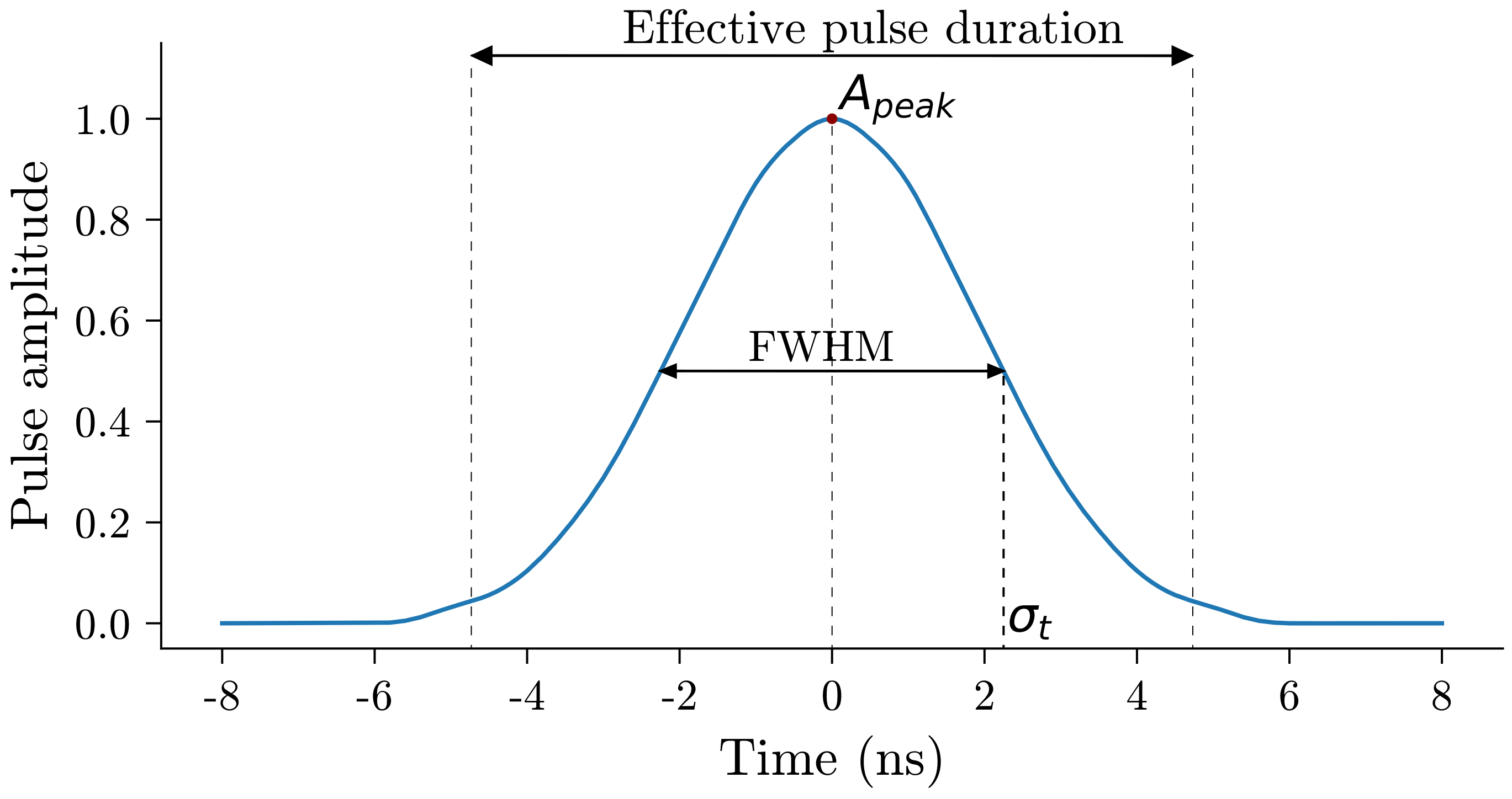
| Half-pulse duration | Laser pulse temporal duration at full-width half-maximum. | 3.5–5.5 ns |
| Pulse repetition frequency | Frequency of emitted laser pulses per second. | 100–400 kHz |
| Scan angle | Maximum laser scanning half-angle from nadir. | 10–30° |
| Scan rate | Number of parallel scan lines per second. | 50–200 Hz |
| Sensor altitude | Platform altitude above ground level. | 400–1500 m |
| Wavelength | Laser operating wavelength. | 1550 nm |
| DART parameters | ||
| Acquisition rate | Temporal interval for digitizing received pulse energy. | 0.5–3 ns |
| Propagation threshold | Minimum pulse energy threshold. Pulse tracking ends when energy ≤ propagation threshold × mean pulse energy. | 0.05–0.15 |
| Scattering directions () | Number of angular directions used to discretize photon scattering [180]. | 60–200 |
| Scattering order | Maximum number of scattering events simulated per pulse. | 5–15 |
| Sub-center photons | Minimum number of rays simulated per sub-cell in each voxel. | 1–15 |
| Voxel size | Resolution of voxels constituting the DART scene. | 0.1–1.0 m |
| Topography | ||
| Slope gradient | Percentage hillslope gradient. | 10–75% |
| Name | Definition | References |
|---|---|---|
| Canopy Cover (%) | Percentage of grid cells at 0.5 m resolution containing vegetation returns above 2 m. | [13] |
| Gap Fraction (Gap) | 1 − (Returns/Returns) | [212,213] |
| Ground return (%) | Percentage of discrete returns classified as ground. | |
| h–h | Height percentiles of vegetation returns above 2 m. | [48] |
| h | Mean height of vegetation returns above 2 m. | |
| Multiple return (%) | Percentage of laser pulses with multiple returns. | |
| Return density | Mean number of discrete returns per m. | |
| Single return (%) | Percentage of laser pulses with single returns. | |
| Canopy volume metrics | Percentage of 1 m voxels classified as Closed gap, Open gap, Oligophotic or Euphotic. | [216,217,218] |
| ALS Metric | Reliability Ratio | Pooled Mean | Pooled SD | Fisher Ratio |
|---|---|---|---|---|
| Return density and laser penetration metrics | ||||
| Canopy Cover (%) | 0.675 | 81.26 | 6.65 | 2.08 |
| Gap Fraction (Gap) | 0.932 | 0.35 | 0.03 | 13.64 |
| Ground return (%) | 0.928 | 34.59 | 3.12 | 12.84 |
| Multiple return (%) | 0.559 | 55.40 | 4.03 | 1.27 |
| Return Density | 0.108 | 18.89 | 5.94 | 0.12 |
| Height metrics | ||||
| h | 0.990 | 11.34 | 0.34 | 100.59 |
| h | 0.971 | 9.35 | 0.55 | 33.15 |
| h | 0.988 | 11.44 | 0.40 | 81.61 |
| h | 0.991 | 12.19 | 0.35 | 114.93 |
| h | 0.995 | 12.96 | 0.28 | 194.48 |
| h | 0.996 | 13.35 | 0.25 | 254.70 |
| h | 0.997 | 13.77 | 0.22 | 340.44 |
| h | 0.998 | 14.79 | 0.18 | 521.11 |
| h | 0.998 | 15.54 | 0.18 | 601.72 |
| h | 0.998 | 16.74 | 0.22 | 413.43 |
| h | 0.994 | 18.05 | 0.35 | 181.95 |
| Canopy volume metrics | ||||
| Closed Gap (%) | 0.913 | 32.67 | 2.62 | 10.44 |
| Euphotic (%) | 0.588 | 14.19 | 2.30 | 1.43 |
| Oligophotic (%) | 0.367 | 18.88 | 3.13 | 0.58 |
| Open Gap (%) | 0.896 | 34.26 | 3.52 | 8.58 |
| Height Percentile | Anderson-Darling | Kolmogorov-Smirnov | ||
|---|---|---|---|---|
| p-Value | p-Value | |||
| h | 0.32 | 0.25 | 0.15 | 0.19 |
| h | −0.29 | 0.47 | 0.14 | 0.26 |
| h | −0.54 | 0.62 | 0.10 | 0.68 |
| h | −0.83 | 0.84 | 0.09 | 0.79 |
| h | −0.89 | 0.90 | 0.09 | 0.79 |
| h | −0.87 | 0.87 | 0.10 | 0.68 |
| h | −0.94 | 0.95 | 0.10 | 0.68 |
| h | −0.99 | 1.00 | 0.10 | 0.68 |
| h | −0.88 | 0.89 | 0.11 | 0.55 |
| h | −0.74 | 0.76 | 0.14 | 0.26 |
© 2020 by the authors. Licensee MDPI, Basel, Switzerland. This article is an open access article distributed under the terms and conditions of the Creative Commons Attribution (CC BY) license (http://creativecommons.org/licenses/by/4.0/).
Share and Cite
Roberts, O.; Bunting, P.; Hardy, A.; McInerney, D. Sensitivity Analysis of the DART Model for Forest Mensuration with Airborne Laser Scanning. Remote Sens. 2020, 12, 247. https://doi.org/10.3390/rs12020247
Roberts O, Bunting P, Hardy A, McInerney D. Sensitivity Analysis of the DART Model for Forest Mensuration with Airborne Laser Scanning. Remote Sensing. 2020; 12(2):247. https://doi.org/10.3390/rs12020247
Chicago/Turabian StyleRoberts, Osian, Pete Bunting, Andy Hardy, and Daniel McInerney. 2020. "Sensitivity Analysis of the DART Model for Forest Mensuration with Airborne Laser Scanning" Remote Sensing 12, no. 2: 247. https://doi.org/10.3390/rs12020247
APA StyleRoberts, O., Bunting, P., Hardy, A., & McInerney, D. (2020). Sensitivity Analysis of the DART Model for Forest Mensuration with Airborne Laser Scanning. Remote Sensing, 12(2), 247. https://doi.org/10.3390/rs12020247